Article

Customer Churn in Retail E-Commerce Business: Spatial and Machine Learning Approach

by
Kamil Matuszelański
and
Katarzyna Kopczewska
*
Faculty of Economic Sciences, University of Warsaw, 00-927 Warszawa, Poland
*
Author to whom correspondence should be addressed.
J. Theor. Appl. Electron. Commer. Res. 2022, 17(1), 165-198; https://0-doi-org.brum.beds.ac.uk/10.3390/jtaer17010009
Submission received: 8 October 2021 / Revised: 5 January 2022 / Accepted: 12 January 2022 / Published: 15 January 2022

Abstract

:
This study is a comprehensive and modern approach to predict customer churn in the example of an e-commerce retail store operating in Brazil. Our approach consists of three stages in which we combine and use three different datasets: numerical data on orders, textual after-purchase reviews and socio-geo-demographic data from the census. At the pre-processing stage, we find topics from text reviews using Latent Dirichlet Allocation, Dirichlet Multinomial Mixture and Gibbs sampling. In the spatial analysis, we apply DBSCAN to get rural/urban locations and analyse neighbourhoods of customers located with zip codes. At the modelling stage, we apply machine learning extreme gradient boosting and logistic regression. The quality of models is verified with area-under-curve and lift metrics. Explainable artificial intelligence represented with a permutation-based variable importance and a partial dependence profile help to discover the determinants of churn. We show that customers’ propensity to churn depends on: (i) payment value for the first order, number of items bought and shipping cost; (ii) categories of the products bought; (iii) demographic environment of the customer; and (iv) customer location. At the same time, customers’ propensity to churn is not influenced by: (i) population density in the customer’s area and division into rural and urban areas; (ii) quantitative review of the first purchase; and (iii) qualitative review summarised as a topic.

1. Introduction

Maintaining high customer loyalty is a common challenge in business. Multiple studies [1,2,3] have proved that retaining customers is more profitable than acquiring new ones. Customer Relationship Management (CRM) deals with loyalty, or oppositely, churn prediction. Most of the previous studies have been conducted for industries in which customers are tied with contracts (such as telecom [4] or banking), which limits the churn rate. Many studies show that customer churn can successfully be predicted using a Machine Learning approach [5,6,7].
We identified a few gaps in the literature which pose challenges that need to be addressed. The first issue is the need to predict churn for an industry where a minor share of customers (single figures, e.g., 3%) stay with the company and buy next time—in many sectors as telecom or banking, the situation is opposite, and the churn rate is 2–3% [8]. The second task is to predict customer loyalty without using a detailed history of the customer but based only on their first transaction [9]. Thirdly, there is a need to study the situation when customers are not bound by a contract and data comes from an online store [10]. The fourth task is to include a spatial dimension—customers’ locations and their neighbourhood characteristics [11]. Finally, textual information from text reviews should be taken into account. These issues are poorly covered in the literature, are not discussed in overview papers [12,13] and have never jointly appeared in a single paper.
This paper studies how to predict customer (un)loyalty, and the goal of the paper is to build and test a comprehensive churn model for e-commerce businesses. We have addressed and covered all of the research gaps mentioned above, and we hypothesise that all information regarding behaviour, demographic and perception features is important for clarifying the determinants of churn. We have tested a few explanatory factors present in the literature: the value of the first purchase [3], categories of products bought by the customer [14], customer location [15], geodemographic data [16], whether the location of the customer is rural or urban [17], as well as the review provided by the customer [18,19]. We used machine learning methods that have been studied for their usefulness in this context. Two classification algorithms were tested—XGBoost and logistic regression. To obtain meaningful information from the text reviews, we applied three topic modelling techniques using a generative statistical approach and neural network modelling. We explain the influence of variables on the target in the case of XGBoost modelling with XAI techniques, even if it looks like a black-box model. To assess the importance of particular sets of features, permutation variable importance was applied to determine the strength and direction of the influence—the partial dependence profile technique.
In an empirical example, we use e-commerce data from a retail shop operating in the Brazilian market. The primary dataset used was shared publicly by the company Olist and contained very detailed information about 100,000 orders made in the store from 2016 to 2018. Available variables in the dataset included the value of the order, products purchased, textual review of the order and customer location. This dataset was enhanced by adding information from Brazil Census data at a very detailed spatial level. Thus, customer orders were combined with customer locations to obtain information about their geo-socio-demographic environment. In the data analysed, nearly 97% of the customers did not decide to make a second purchase.
There are sound implications of this research. From a theoretical perspective, the paper establishes a new approach in CRM studies. It shows that churn modelling is also feasible with scant data, with almost no history on customer behaviour and no contracts with customers. It also opens CRM to external information, especially the customer’s geolocation and their socio-economic environment. Those features may have important practical implications. First, they open the path for quick online CRM systems, which can label customers as “potentially loyal” already at their first purchase. Secondly, they increase the importance of big data analytics and combining different data sources, also those seemingly unrelated such as census data and neighbourhood socio-economic features. Third, they may save time by showing that machine learning models calibrate faster than logistic regression, while textual reviews, which are time-consuming in processing, may not give added value in churn prediction.
This paper is structured as follows. It first reviews existing studies regarding customer churn prediction, methods applied in this area and the selection of input data. Secondly, it presents quantitative analytical methods used for pre-processing, topic modelling, variable selection and churn modelling, offering Natural Language Processing (NLP), Machine Learning (ML) and Explainable Artificial Intelligence (XAI) tools. Thirdly, it presents a dataset overview from a transactional and spatial perspective. Fourth, it describes the results of pre-processing, performance analytics and XAI usage. We close the paper by discussing the possibilities for future research and our conclusions.

2. Customer Churn in CRM and Modelling—Literature Review

Customer Relationship Management (CRM) is defined as a process in which the business manages its interactions with customers using data integration from various sources and data analysis [20]. There are four questions which CRM approaches can be used to answer [21]: (1) Customer identification (acquisition)—who is a potential customer? (2) Customer attraction—how can one make this person a customer? (3) Customer development—how can one make a customer more profitable? (4) Customer retention—how can one make the customer stay with the company? The last one, customer retention, is the main focus of this study.
Improving the loyalty of the customer base is profitable to the company. This has its source in multiple factors, where the most important one is the cost of acquisition. Numerous studies have proved that retaining customers costs less than attracting new ones [1,2,3]. Moreover, there is some evidence that loyal customers are less sensitive to competitor actions regarding price changes [22,23].
There are two basic approaches for companies dealing with customer churn. The first one is an “untargeted” approach. This is where a company seeks to improve its product quality and relies on mass advertising to reduce the churn. The other method is a “targeted” approach, where the company tries to aim their marketing campaigns at the customers who are more likely to churn [24]. This approach can be divided further by how the targeted customers are chosen, for example, the company can target only those who have already decided to resign from another relationship. In contractual settings, this can mean cancelling a subscription or breaching a contract. Another way to approach the churn problem is to predict which customers are likely to churn soon. This has the advantage of having lower costs, as the customers who are about to leave are likely to have higher demands from any last-minute deal proposed to them [10].
A literature review demonstrates [10] that most studies concerning churn prediction have been performed in contractual settings, where churn is defined as the client resigning from using a company’s services by cancelling their subscription or breaching the contract. This way of specifying churn is different from a business setting, where the customer does not have to inform the company about resigning.
One problem that arises in the non-contractual setting is the definition of churn. As there is no precise moment when the customer decides not to use the company’s services anymore, it must be specified by the researcher based on the goals of the churn analysis. One can label customers as “partial churners” when they do not make any new purchases from the retail shop for three months [21]. In other approaches, “churners” are all the customers who have a below-average frequency of purchases [3] since these customers have been shown to provide little value to the company. In the case of this study, customers were classed as churners if they never bought from the shop again after their first purchase.

2.1. Quantitative Methods in Customer Churn Prediction

Customer churn prediction is a core issue for businesses. If a company can successfully predict who may leave, it can then target those customers with a retention-focused campaign, which is much cheaper than targeting all customers. From a technical perspective, churn prediction is a typical classification task, as the variable to predict is binary (churn or no churn). However, such binary prediction is not as valuable for later retention campaign efforts. It is equally important that the machine learning model can predict the likelihood of the customer leaving [25] and help build a ranking of the customers from the most to the least likely to churn. This churn likelihood ranking is very attractive for businesses. First, the company can decide what percentage of customers to target in the retention campaign and they are not bound by how many customers the model will predict as potential churners. Second, the company can decide how strong the targeting should be based on the likelihood to leave. For example, based on cost-benefit analysis of various targeting approaches, one could decide that for the top 10% of the “riskiest” customers, the company will offer big discounts on their next purchase, while for the top 30% they would only send an encouraging email. The churn prediction task can be decomposed into two main important aspects to tackle. The first is to find a specific machine learning model that gives the best performance, and the second is to decide on the model formula—which variables to include and what form of relationship to apply.
Machine learning models have gained importance in churn prediction (overview in [12,26]). The two most widely used techniques are Logistic Regression (LR) and Decision Trees (DT), which are relatively simple [27]. However, they often give sub-optimal results compared to more advanced and recent approaches like Neural Networks (NN) or Random Forests (RF) [21,28]. This is true in churn predictions and also in more general applications using multiple datasets and comparison metrics [29]. Recently, the Extreme Gradient Boosting (XGBoost) algorithm [30] has gained popularity in numerous prediction tasks. XGBoost’s main strengths are inferring non-linear relationships from data and its relative speed, which allows the researcher to try out multiple hyper-parameters and decide on the best ones [30]. Because of these factors, XGBoost is considered a go-to standard for machine learning challenges, and very often, solutions based on this algorithm achieve the best results in various competitions and compared to benchmarks [31]. In the context of churn prediction, XGBoost was used by [7]. It achieved superior performance compared to other techniques, specifically logistic regression and random forests.
In quantitative analyses, one needs both good predictions as well an understanding of what factors drive these predictions. While deciding on the type of machine learning algorithm, one usually faces a trade-off between explainability and performance [32]. More flexible models such as bagging, boosting or neural networks are often superior to less flexible approaches. On the other hand, their predictions cannot be explained as quickly, as in the case of, for example, decision trees or linear regression. A solution for this problem is Explainable Artificial Intelligence (XAI), which is a set of tools aimed at explaining predictions of these highly flexible models. Thus, it transfers the advantages of simple models to flexible models to provide superior performance [33].
Recently, machine learning models have been judged against a set of criteria in deciding the best accuracy [34]. These criteria include (a) fairness—whether the algorithm is biased against a particular gender, age, race, etc.; (b) robustness—whether the algorithm can provide correct predictions when the parameters change; and (c) trust—whether the final users of the algorithm trust the model’s predictions. When deciding on which methodology to apply, machine learning practitioners must assess which of the above requirements are essential in a particular task. For example, in CRM settings, trust in the model’s predictions is much less critical than in medical areas but can still be crucial for broad adoption of modelling across a company. Similarly, sometimes explainability will only be important for the person developing the model to understand its limitations and be able to improve upon them. The XAI tools can help address the issues mentioned above without sacrificing the usual performance gain from black-box models.
Research on explainable artificial intelligence in the marketing domain is not very developed, with only a few papers published on this issue [35]. One can specify potential areas for future research in this field [35], including: (a) understanding the acceptable requirements regarding explainability compared to accuracy in different marketing tasks, (b) making AI trustworthy, including understanding how the adoption of an AI system’s predictions increases in a company when various explainability tools are made available to the end-users, and (c) how model explanations should be presented to various groups of a system’s users. For example, a machine learning expert is interested in very detailed and complex explanations, while a company’s customer may simply want a one-sentence summary of what was considered while making predictions.
Machine learning models are useful not only in CRM analytics. An important source of knowledge comes from textual reviews, which can potentially serve as a rich source of information about customer satisfaction. Although text mining for customer reviews is, in general, an active field of research, usage of such information in the context of churn prediction is much less covered. Two existing papers on using textual reviews for churn prediction apply an embedding approach [19] and a simple tf-idf technique [36]. Two natural language processing methods are usually used to extract insights from customer reviews [37], which are topic modelling, i.e., “what is the review about?”, and sentiment analysis, i.e., “what is the perception presented by this review?” Combining these two dimensions can help show which areas of customer experience are rated positively, and which need improvement. In the case of this study, the focus is only on extracting the topic from the review, as information about whether the customer’s experience was positive or not is already contained in a numeric review. We aimed to test whether customer perception expressed both in a numeric review and a textual review act as valuable predictors of customer loyalty.

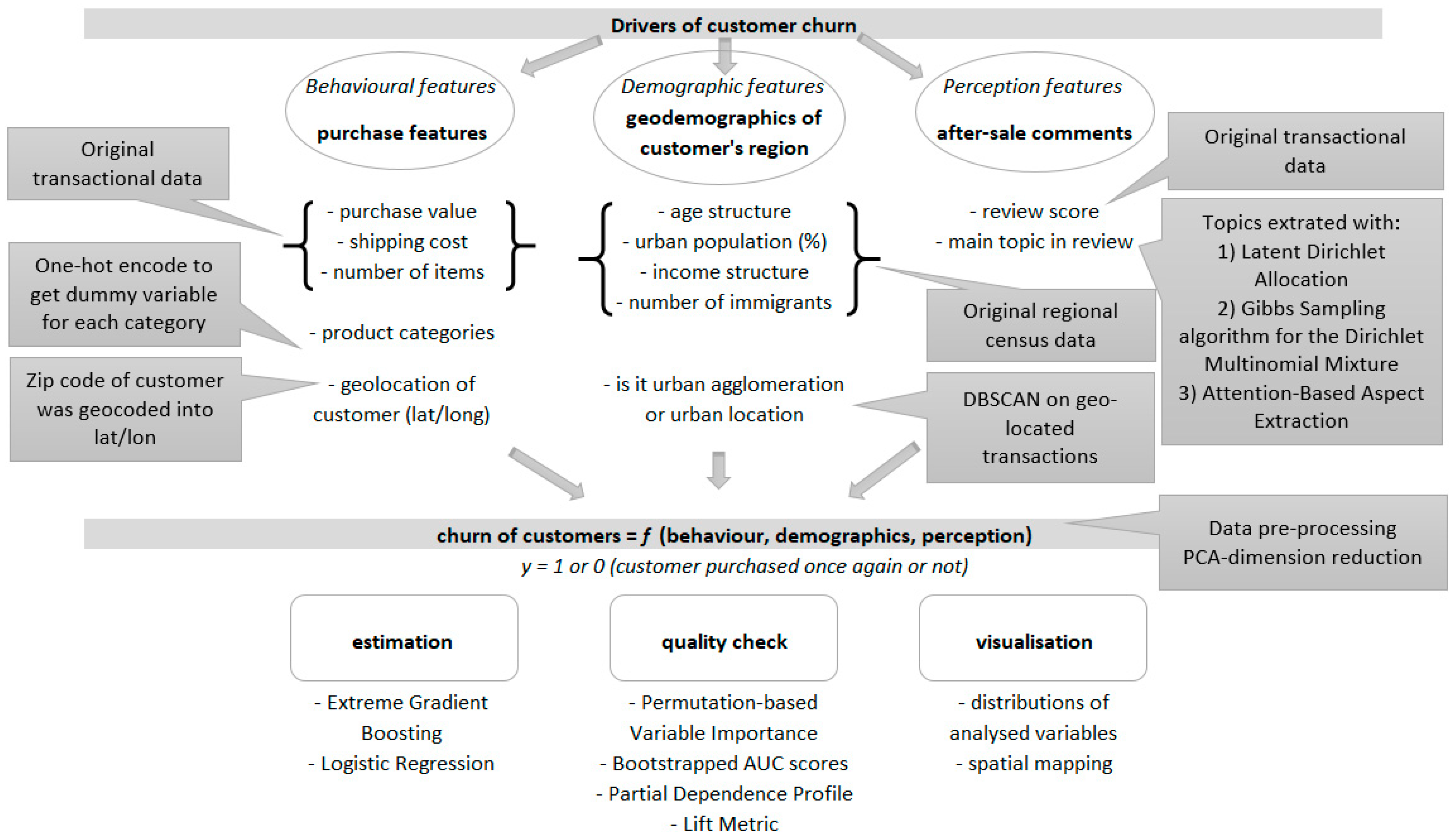
2.2. Information Used in Churn Prediction

The selection of appropriate variables to analyse churn prediction is essential. It provides the basis for creating the best-performing model and for gaining insight into the factors which influence customer churn, which can be used in other areas of CRM. Previous churn prediction studies included a wide variety of variables in their model formulation. They can be divided into three broad categories [3]:
  • Behavioural—describing how the customer has interacted with the company previously.
  • Demographic—describing the customer in terms of their inherent characteristics, independent of their interactions with the company.
  • Perception—describing how the customer rate their previous interactions with the company.
The studies in which these sets of variables have been used are reviewed below.
Behavioural features can be defined as variables which quantify the previous actions of a customer. In most cases, this narrows down to the data about previous transactions with the company. This information is easy to obtain in most companies, as it is needed for accounting purposes and is often already analysed in other company areas. Moreover, variables such as transaction value are understandable even by non-experts. Such data were shown to be an important predictor in churn prediction in multiple studies (overview in [38]). Typical features in this category are recency, frequency and monetary value, which constitute the basis of the RFM customer segmentation framework. These features are used in multiple studies [3,21,39] and typically accompany more complex variables encompassing frequency and monetary value or total spending divided by the categories of the products available in an e-commerce shop [3]. The literature proves that these variables are statistically significant and improve the model’s predictions [3,4]. It is also known that bigger customer spending leads to the customer’s desire to continue being a customer and that the previous purchase categories influence the customer’s decision to stay [3,14,40]. One possible explanation of churning based on purchased categories is that the satisfaction of buying a particular class is low—and is not related to a high price or low quality of the product bought [14]. In this study, in the context of e-commerce retail, we wanted to check if the amount of money spent on the first purchase positively influences the customer’s probability of buying for the second time, and if categories of purchased products affect the customer’s probability of staying with the company.
Demographic and location features of customers describe age, gender or address. They have been shown to be good predictors of customer churn in multiple studies (overview in [26]). However, the availability of such predictors to use in modelling is very often limited for various reasons. In non-contractual settings, it may happen that customers do not provide such data to the company. Moreover, using such personal data can be considered unethical and can lead to predictions biased against a particular race, age or gender. In this study, the only demographic feature available is customer location, as neighbourhood can be an important factor to consider in CRM analyses [41]. There are multiple ways to include this kind of spatial information in modelling churn prediction. In this study, three approaches were applied: (a) directly including location variables (geographical coordinates, zip code or region indicator dummies); (b) analysing the neighbourhood that the customer resides in (demographic statistics about the region); and (c) classifying customers by living in an urban or rural area. Details and justifications are presented below.
Direct inclusion of spatial variables has not before been presented in churn prediction literature, and this is the first study that includes raw geographic coordinates in the model formulation. It is more common for researchers to include dummy variables indicating administrative regions. There is no consensus on whether such data can improve predictions, as one can argue [42] that “the number of times a customer called the help desk will most probably be a better predictor of churn behaviour than the zip code”. On the other hand, such dummies have shown significance in neural network models but not in random forest models [3,15]. However, different spatial information was analysed in that case—the region variables indicated countries rather than postcodes. Geolocation data can also be used in the example of churn prediction for an insurance company [43] for operationalising customer location; instead of including dummies indicating the customer’s region, one can calculate the distance between the customer and the closest insurance agent. Such variables have been shown to be significant. In this study, we checked if the propensity to churn can be explained directly by customer location.
Geodemographics is the “analysis of people by where they live” [44]. In this paradigm, it is assumed that people living in the same area share similar characteristics, like their social status and income, etc. Geodemographic features have mostly been used in public sector areas, mainly in public health and law enforcement [45]. Publicly available research on the usage of geodemographic in marketing, or specifically churn prediction, is almost non-existent due to the confidential nature of research performed by individual companies [46]. The only publicly available study [16] shows that geodemographic features obtained from census data were significant in the churn prediction model. In this study, we check if the demographic and social structure of a customer’s environment can serve as a valuable predictor of churn tendency.
Rural and urban customer location is commonly treated as a variable diversifying customer behaviour [47]. In particular, a couple of studies in the FMCG sector have found that rural customers tend to be more loyal to their previously chosen company [17,48]. One potential reason for such a finding is that there is a smaller number of other options in rural shops than in urban ones. However, to date, there are no e-commerce studies which assess the differences between customer loyalty in urban and rural areas, and the findings from the FMCG sector do not translate directly because customers are not generally limited by the availability of a brand in their area in an online setting. In this study, we will check if the tendency to churn is dependent on whether the customer is living in a densely populated area, which is a good proxy of a rural or urban location.
Customer perception of the company is considered an important factor driving customer loyalty [18]. Unfortunately, customer satisfaction is a variable difficult to measure. Different proxies can be included in the model, and usually gathering such data requires conducting customer surveys. There are various possible dimensions of such a survey, including “overall satisfaction, quality of service, locational convenience and reputation of the company” [21]. In e-commerce settings, an industry standard is to provide a way for customers to express their opinions about their purchase [37]. The company has to decide in a structured way of how it would like to collect these reviews. Text reviews can provide richer information about the customer experience, and they are not limited to describing the experience in predefined dimensions. On the other hand, extracting meaningful information from potentially millions of text reviews is a challenging task to which no universally acclaimed solution exists [49,50].

3. Methods Used in the Analysis

We tested the impact of various predictor variables on customer churn. We applied machine learning modelling, which requires the following steps:
  • Pre-processing the variables present in the dataset so that they can be included in the model.
  • Defining the machine learning modelling methods to be used, in particular choice of the metric to be optimised and the type of model.
  • Training the model using various sets of variables, and the selection of independent variables which maximise the performance of the proposed model.
  • Running the predictions from the selected models.
  • The methodology used in this study can be divided into four broad categories:
  • Methods used in pre-processing applied to the variables present in the dataset.
  • Methods used for variable selection.
  • Machine learning modelling methods—choice of model, cross-validation, up-sampling, etc.
  • Methods used to check the strength of the variable’s influence.
Below we describe the details of these methods. Figure 1 presents an overview of the whole analysis.

3.1. Data Pre-Processing

Pre-processing, applied to all the dataset parts, can be structured as a flowchart (Figure 2). All of the tables on the left-hand side come directly from Olist (4 tables) and Statistical Office sources (1 table—demographic data). The purple table is the primary one, and the features from this table were combined with all the remaining sets of variables. The final tables created after pre-processing each of the parts of the dataset are shown in grey. In the modelling phase, we performed a simple join of the basic table and the remaining tables (e.g., basic information + order items; basic information + DBSCAN cluster, etc.).
In this study, we pre-processed three separate groups of variables: behavioural (first transaction) features, location features and perception features, described in detail below.
Behavioural features of customers were derived from the monetary value of the first purchase, delivery cost, number of items bought and the categories of the purchased items and were included in the model formulation. The value of the purchase, as well as the product category, were of central interest, as they have been shown to be significant in other studies on customer churn. The purchase value was directly inserted into the model as it did not require any pre-processing. In the case of the product category, two steps were taken. First, some of the products were very rare in the dataset, and thus were binned into one category because of potential problems with generalisation and slower model training. Secondly, this variable needed to be converted to a numeric format. Thus, all product categories except the top 15 most popular ones (responsible for 80% of purchases) were binned as a new category “other”, then, one-hot encoding was utilised to create a numeric representation, with the “other” category set as a base level. One should remember that there can be multiple product categories in one order, so it was not guaranteed that there would be only one “1” entry per row, as in the classical one-hot-encoding method.
Location features were included in three ways. Firstly, we wanted to assess if the propensity to churn could be explained by customer location; thus, the model formulation directly comprised longitude/latitude data about each customer. Secondly, we used in total 35 geodemographic features for the micro-region where the customers were based, including age structure, percentage of the population in an urban area, income structure and number of immigrants. These features helped to check if the social structure of the customer’s environment can serve as a valuable predictor of churn tendency. Combining the data sourced from the population census and the main transaction dataset proved to be challenging. The details of such spatial join are presented in Appendix A. The geodemographic dimensions in this study were relatively high (for example, there were 20 variables encoding only age structure), and as some variables provided repeat information, we compressed the data using principal component analysis. This brought some improvements in the process of machine learning modelling (as in other studies, e.g., [51]), because training the model on a smaller, compressed dataset is more resource efficient. One decision we were faced with regarding PCA transformation was whether to use a standard version or rotated loadings [52]. The trade-off between these two methods is that the rotated loadings version allows for an interpretation of the loadings but is less optimal because the variance along each loading is not maximised. The standard version is more suitable in the case of this study because the explainability of the input variables to the model is not as important as correctly representing the features in a lower-dimensional space, thus preserving as much valuable information as possible for the modelling phase.
Thirdly, we included information on whether customers lived in a rural or urban location, which can be extracted using two methods. One method checks if the customer’s coordinates are inside the city’s administrative boundaries. Such an approach does not guarantee that this customer is really living in a densely populated area—because administrative and actual boundaries may not overlap (e.g., because of fast suburbanisation and spillover from the city to previously village areas).
The second method infers the population density in the area from empirical data. This method provides classifications that better reflect reality in densely populated areas. In our dataset, the number of customers per micro-region correlated highly with population density in this area. Because of this, it could be argued that in analysis that uses a smaller scale than micro-regions, such correlation would also be evident. This leads to a conclusion that customer location can be used as a proxy for population density in order to classify densely and sparsely populated areas. Even if this is not valuable for churn modelling, this information can be appended into CRM system tables and applied to other customer analyses. Technically, one of the best and most commonly used algorithms to detect high- and low-density areas, thus rural vs. urban classification, is the density clustering method DBSCAN (Density-Based Spatial Clustering with Noise). In this method, points intuitively form a high-density cluster, while other points densely fill the surrounding, and in contrast, the points which in the neighbourhood do not have many different points are considered as noise. The DBSCAN algorithm has two parameters to set. These are the minimum number of points lying close to each other that are needed to constitute a cluster (k) (number of points to find in a given radius), and the maximum distance that one considers the points to be close to each other (ϵ) (radius, which forms the circle within which one counts neighbouring points). A detailed DBSCAN algorithm works as follows:
  • Create the list points_to_visit with all the points from the dataset.
  • Assign all points as noise.
  • Select a point x randomly from points_to_visit and remove it from the list. Check how many points have a distance to it less than ϵ. If this number is more than k, a new cluster is created that includes all these points. Assign all these points to a list cluster_points. For each of the points from this list, repeat recursively step 3 until cluster_points does not contain any points.
  • After creating the previous cluster, select the next random point from points_to_visit and repeat step 3 until all points have been visited.
DBSCAN, besides the assignment of points to a particular cluster, can also detect noise points. Because of this, the assignments have a natural interpretation. When a point belongs to any cluster, this customer lives in a densely populated area. In contrast, the points decoded by DBSCAN as noise are the customers living in more isolated (rural) places. A typical rule-of-thumb for deciding k and ϵ (epsilon) parameters is to first set k, and then plot k-nearest-neighbours (knn) distance. Epsilon should then be determined based on the elbow point, where the line bends. In this work, the minimum number of customers in the cluster was set to 100, and the maximum distance between the customers in one cluster was set to 50 km. In relation to the location of Brazil on the globe, this transfers roughly to epsilon =0.2.
The last category of data, perception features, were proxied by reviews through: (a) numeric assessment on a scale from 1 to 5; (b) textual review of the purchase. These two features can help check whether customer satisfaction is an important factor in churn prediction. Using numeric reviews in the modelling was straightforward and does not require further explanation. However, the textual reviews required intensive pre-processing (details described below). This study is a first attempt to use the topics inferred from reviews in churn prediction. Similarly, as with the rural vs. urban area indicator described before, generated review topics can help other CRM efforts. For example, the topics of reviews can be included in a review monitoring system and enable marketing specialists to analyse customers’ reviews in a more automated manner.

3.2. Methods for Topic Modelling

Customers’ reviews are usually short texts, and for CRM analysis, one needs to extract the topic (aspect). The most popular model for inferring the topic of a text is Latent Dirichlet Allocation [53]. The method is based on the assumption that each document is a mixture of a small number of topics. At the same time, each topic can be characterised by a distribution of word frequency. However, short texts (such as customer reviews) comprise a very small number of topics, usually only one [54], and because of this, LDA should not be used in such settings as its assumptions are violated [55]. This was confirmed by an empirical study of short texts from Twitter, in which LDA failed to find informative topics. An alternative and improved method over typical LDA is the Dirichlet Multinomial Mixture model, applied jointly with the Gibbs Sampling algorithm [55]. The main difference lies in the assumption that each text comprises only one topic, making DMM superior to LDA in short texts. Another innovative alternative to LDA and which is a milestone in the whole NLP field is word2vec [56], which is an efficient way to embed words in a vector space while preserving their meaning. This method became a basis for the Attention-based Aspect Extraction model [57]. In empirical research, algorithms based on word embeddings outperform LDA in the task of short text topic modelling [58,59].
In this study, three algorithms for topic modelling were tested and evaluated:
  • Latent Dirichlet Allocation [53]—because it is a go-to standard for topic recognition.
  • Gibbs Sampling algorithm for the Dirichlet Multinomial Mixture [55]—this method is an improvement over LDA, intended primarily for short texts. This is relevant for this case, where most of the reviews were just a couple of words long.
  • Attention-Based Aspect Extraction [57]—this method is also meant for short texts, and at the same time, it uses the most modern, state-of-the-art NLP techniques. Furthermore, in the original paper, the authors worked in a similar domain of internet text reviews.
After applying each of these methods, one can obtain assignments of each of the reviews to a topic. Such assignment can then be one-hot encoded and included in the model specification. Details of each method are described below.
Latent Dirichlet Allocation (LDA) is a generative statistical model with assumptions as follows:
  • Consider a text corpus consisting of D documents. Each document D has N words that belong to the vocabulary V. There are K topics.
  • Each document can be modelled as a mixture of topics. Document D can be characterised by the distribution of topics θ_D that come from the Dirichlet family of probability distributions. Each topic has a distribution of words φ_k which come from the Dirichlet family. Then, a generative process aimed at obtaining document D of the length of N words w_(1, …, N) is as follows:
  • To generate a word at position i in the document:
    Sample from the distribution of topics θ_D, and obtain an assignment of word w_i to one of the topics k = 1, …, K. This is to obtain information from which of the topics the word should be sampled.
  • Sample from the distribution of words in topic φ_k, and obtain the word to be inserted at position i.
The parameters of θ_D for each document D, as well as φ_k for each of the topics, should be learned using some method of statistical inference. Most of the practical implementations of the algorithm are based on the Expectation-Maximisation method. This iterative approach aims to find the local maximum of the likelihood function for the analysed dataset.
Gibbs Sampling algorithm for the Dirichlet Multinomial Mixture is very similar to the LDA approach with the difference that each document includes words from only one topic. This assumption is based on the authors’ claim that usually, in the case of short texts, only one topic is present. This leads to the following generative process. To generate a document D:
  • Sample from the distribution of topics θ_D and obtain an assignment of the document to one of the topics k = 1, …, K.
  • Sample all words from the topic distribution φ_k.
Attention-Based Aspect Extraction takes a very different approach to topic modelling compared to the methods above. It is not based on a statistical model but rather on neural network modelling. The following steps describe the model architecture presented visually in Figure 3. For each document from the corpus:
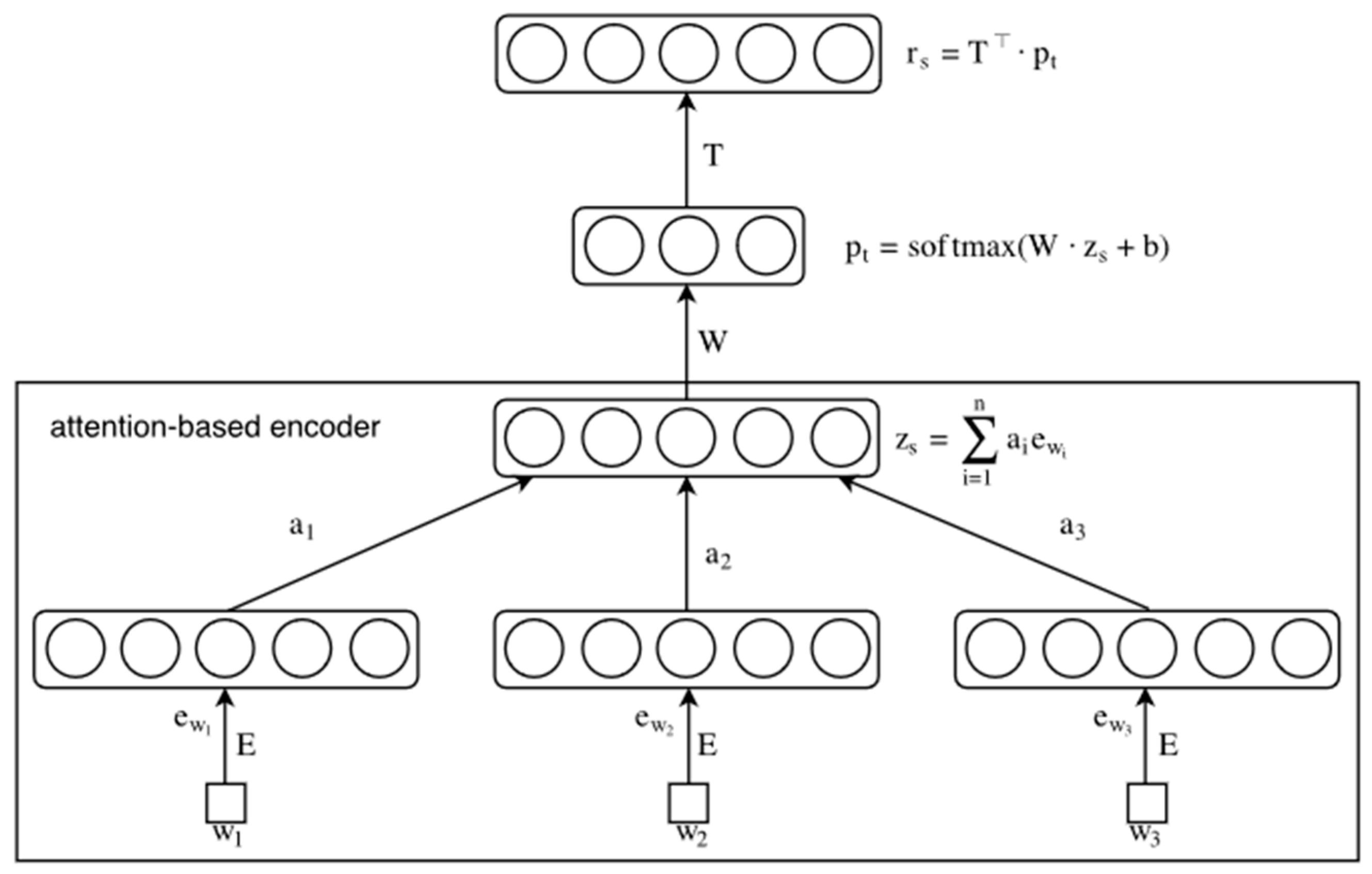
  • Calculate the word embeddings e_(w_1), e_(w_2), e_(w_3), … with dimensionality d for each of the words from the vocabulary based on the whole corpus. From this point, one obtains an assignment of the word w to the feature vector e_w in the feature space R^d.
  • Obtain document embedding z_s. This is done by averaging the embeddings of all the words from the document. The average is weighted by attention weights a_1, a_2, a_3 given to each of the words. These weights are estimated during the model training and can be thought of as a probability that the particular word is the right word to focus on to infer the document’s main topic correctly. It is worth noting that the document embedding shares the same feature space as the word embeddings.
  • Then, calculate p_t using softmax non-linearity and linear transformation W. This vector p_t is of the same dimensionality as the number of aspects to be learned and can be thought of as a representation of the probability that the sentence is from the particular aspect. By taking the biggest probability of this vector, one can obtain the assignment to the particular topic.
  • Increase the dimensionality of the vector p_t to the original dimensionality d by transforming it with aspect matrix T. Vector r_s is obtained.
  • The training of the model is based on minimising the reconstruction error between the vectors z_s and r_s.
This method can capture better, more coherent topics than LDA and its equivalents. The main specified reason is that in LDA, all of the words are assumed to be independent; thus, information about the “closeness” of the meanings of words is lost and has to be learned by assigning similar words to the same topics. This is a challenging task that LDA is not optimised for. On the contrary, using the word embedding approach, the models’ relationships are known a-priori by the model and can be built upon. For example, even without knowing the topics present in the corpus, one would expect that the words “cow” and “milk” should indicate the same topic with high probability. Such information is present in the word embeddings that this method uses.
All three algorithms require various types of data pre-processing. There are a few common actions for all algorithms:
  • Translation of the reviews from Portuguese to English. The Olist e-commerce store operates only in Brazil, which is why most of the reviews are written in Portuguese. Google Translate API was used to change their language to English. This is not only to facilitate understanding of the reviews, but also because NLP tools available for the English language are more advanced than for other languages.
  • Removal of stop-words and punctuation.
  • Lemmatisation using WordNet lemmatizer [60] combined with a Part-of-Speech tagger. This step is needed to limit the number of words in the vocabulary. Thanks to the Part-of-speech tagger, the lemmatizer can change the form of the word on a more informed basis and thus apply correct lemmatisation to more words.
Later steps of the pre-processing were different for each of the algorithms.
For LDA and Gibbs Sampling, converting the lemmatised reviews into vector format was sufficient. In the case of LDA, the count-vectorising approach was applied, removing words that appeared in less than 0.1% of reviews. In the case of Gibbs Sampling, the same pre-processing was performed internally by the training function from the package. After vectorisation, in both cases, one should obtain a matrix with n rows and k columns, where n is the number of observations in the original dataset, and k is the vocabulary size.
Very different pre-processing was required in the case of attention-based aspect extraction. The neural network architecture proposed by the authors simply requires lemmatised reviews in a textual format as the input. Then, one of the layers of the network is meant to embed the currently pre-processed word. These embeddings are not learned during the network training; they should be trained beforehand instead. The authors of the paper propose the word2vec technique [56] for learning embeddings. Following their guidelines, this paper uses this method, with the dimensionality of the vector space set to 200 and the word window set to 10. After applying word2vec on this dataset, a matrix with m rows and 200 columns was obtained, where m stands for the number of words in the dataset, and 200 is the dimensionality of the vector space chosen as a hyper-parameter.
Concerning topic modelling training, optimal hyper-parameters for all three models were tested based on a grid search. For LDA, different numbers of topics were tested (3, 5, 10 and 15). For GSDMM, two parameters influenced topic coherency in each “cluster”. The algorithm was run for all 16 combinations of both parameters chosen from the values 0.01, 0.1, 0.5 and 0.9. For attention-based aspect extraction, the different numbers of topics to learn was tested, using the values 10 and 15. Unfortunately, as this last model takes a very long time to run (around 3 h per one set of hyper-parameters), the number of hyper-parameters checked needed to be limited.
The evaluation of topic extraction is a complex task, as no model-agnostic metrics which compare different models exist. The only reasonable method is human inspection. This is why after running every model, the obtained topics were verified for coherency (whether the reviews inside one topic are similar) and distinctiveness (whether there are visible differences between modelled topics). In the modelling phase, only one-hot encoded topics obtained from the best model were used.

3.3. Variable Selection Methods

The data pre-processing stage transformed data into the input form. However, the inclusion of variables in the final models needed to be justified—from a theoretical point of view or using variable selection methods. This helps to build a more coherent model and increases computational efficiency. In this study, variable pre-processing produced six sets of features:
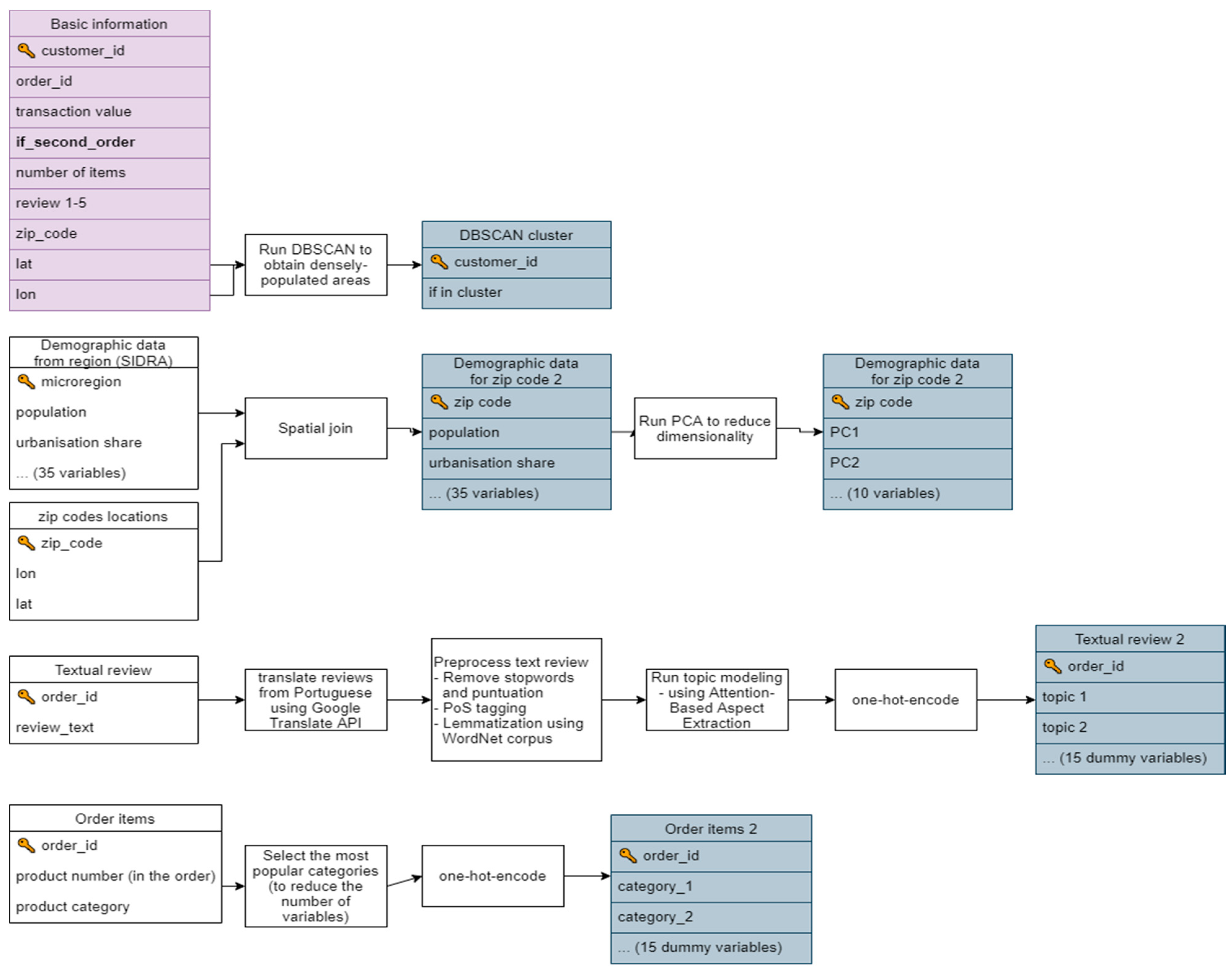
  • Basic information: the value of the purchase, geolocation in raw format lat/long, shipping cost, number of items in the package, review score (six variables).
  • Geodemographic features for the region where the customer is based: age structure, percentage of the population in an urban area, income structure, number of immigrants (35 variables).
  • Geodemographic features transformed using PCA (10 variables/components).
  • An indicator of whether the customer is in an agglomeration area obtained from DBSCAN location data (one variable).
  • Product category that the customer has bought from in prior purchase (15 dummy variables).
  • The main topic that the customer mentioned in their review (15 dummy variables).
Some of these variables are already well known in CRM literature and have been proven to work well. However, in the case of new, never-before-tested variables in churn prediction, one should apply a testing procedure [21] to compare two models; one containing only basic RFM features, and the other RFM features together with new features. In this study, we constructed a baseline model which included only basic features that did not require any pre-processing. Then, for each set of computed features, we built a model containing these new features together with the basic features. Lastly, one model was trained which contained all variables. In consequence, we tested seven feature sets:
  • basic features
  • geodemographic + basic features
  • geodemographic with PCA + basic features
  • agglomeration + basic features
  • product categories + basic features
  • review topic + basic features
  • all variables (with geodemographic features transformed using PCA)
It is important to note that the model containing all variables with demographic features without PCA pre-processing was not trained. There are two reasons for this—one is that the number of variables in this set is very big, which poses implications for performance and the model training would take a very long time. The other reason is that the model that only included PCA demographic variables performed better than the full set of variables.
In the selection of features, we applied an automatic approach using the Boruta algorithm [61], which is popular among machine learning practitioners [62]. The algorithm is a wrapper used for feature selection and is built around the random forest algorithm. It works as follows. Firstly, all features from the original dataset are randomly permuted. This way, one obtains a dataset with close to zero predictive power. Then, the resulting features are added to the original dataset and the random forest model is trained. This model has a built-in feature importance measure, which is usually Mean Decrease Impurity (MDI). After running the model for each of the original features, MDI is compared against all MDI scores for shadow features. If the score is less than the one from any of the shadow features for any original variable, the variable gets a “hit”. The above procedure is repeated for a preassigned number of iterations. Finally, essential features that should make it to the final model are the ones that obtain fewer hits than the preassigned value. However, one should remember that the Boruta algorithm is very time-consuming. The minimal number of runs recommended by the method authors is 100, and one run consists of fitting a random forest model to the whole dataset with a doubled number of features (because of added shadow features). The Boruta algorithm fits the model to 2*k features (original and shadow features) in each iteration, and in the case of this analysis, model computation took about 12 h on a modern laptop. Other wrapper algorithms also require an iterative fitting of the model; they usually start with fitting the model to one variable, in the next iteration to one, and so on up to k features.

3.4. Modelling Methods

In this study, we compared two binary regression models: logistic regression and extreme gradient boosting, which find factors distinguishing churn/non-churn behaviour. The reasons for the choice of these particular models are as follows. Logistic regression is relatively explainable and straightforward and has been used in churn modelling in previous studies [5,6]. On the other hand, the XGBoost model has been shown to yield superior performance in all kinds of modelling using tabular data, and in the context of churn prediction [7]. It can also learn non-linearities and interactions between the variables on its own, contrary to LR, where such features should be introduced to the model manually. We expected that XGBoost would give better performance, but at the cost of losing direct explainability.
XGBoost is based on the principle of boosting and works as follows. Firstly, a weak model (typically a classification tree) is fitted to the data. Then, predictions are made using this model and residuals are obtained. The next model is fitted with the original independent variables, but the dependent variable is the residual obtained from the previous model. This is repeated sufficiently many times, and the final output of the model is the prediction made by the last model. In validation, we used a simple train-test split of the dataset, with 70% of the observations belonging to the training dataset. Optimal hyper-parameters were chosen using two-fold cross-validation on the training dataset. The search space is defined as a grid of all possible combinations of the hyper-parameters.
One crucial problem with this dataset is its very high target class imbalance, as only 3% of the customers decided to buy for a second time. To handle this issue, up-sampling of the minority class on the training dataset was used to obtain equal class proportions [8]. Secondly, we carefully selected an appropriate metric to optimise, as some metrics (like accuracy) are very biased against the minority class in these cases. For example, if the dataset contains 99% of observations from the majority class, one can simply use a classifier that always predicts the majority class and obtain 99% accuracy—although none of the observations from the minority class will be classified correctly. For this reason, the Area-Under-Curve (AUC) metric was used, as it weights the performance of the minority and majority classes equally—which is crucial for non-balanced ratios [8,63]. The AUC metric is based on the Receiver Operating Characteristic (ROC) curve. This curve is created by plotting the true positive rate against the false-positive rate for various cut-offs of the response variable, and the AUC metric is defined as the area under the curve of the ROC metric. It has a range between 0 and 1 (the closer to 1, the better). A value of 0.5 means that the model is no better than random guessing—and thus has zero predictive power. A value of 1 is obtained by the model correctly classifying all observations. It is worth noting that using imbalanced metrics should not change the results when the minority class is up-sampled to obtain equal proportions. However, in the case of this study, up-sampling was applied only on the training set. Because of that, although the results for accuracy and AUC on the training set should be similar, AUC is a better choice on the test set. AUC was used in both model training and evaluation on the test set to maintain consistency.
The difference between logistic regression and XGBoost algorithms lies in the explainability of results. Logistic regression is an interpretable model by design—one can simply look at the model coefficients and infer the strength and direction of influence of a particular feature on the final prediction. On the contrary, XGBoost is still a black-box model whose structure is too complex to be directly inspected—even if some progress in explainability and transparency of results has been done [64]. When checking the importance and direction of influence of variables for model prediction, novel Explainable Artificial Intelligence (XAI) techniques have to be employed. Using such an approach can also help gain intuition about what features the loyal customers have in common. In this study, we used two XAI techniques: Permutation-based Variable Importance (VI) and Partial Dependence Profile (PDP). The first one can help in answering the question “which variables (or categories of variables) influence the predictions the most?”, while the second answers “what is the direction and strength of this influence?”.
Permutation-based variable importance [65] is a model-agnostic method and should be applied to models such as XGBoost, which do not have a model-specific variable importance measure (as, for example, mean decrease gini in the case of random forest). It also allows testing not only feature importance of one variable at a time, but also sets of variables. It is an equivalent of p-value significance in classical econometrics. The method is based on model performance changes when random permutations are applied to predictor variables. Because the feature values are “exchanged” between the observations, they stop bringing any information to the model (because they are random). If the model heavily uses a particular feature in obtaining predictions, then the model’s performance will drop by a large amount. Similarly, if the model does not use a feature at all, the model’s performance will not change when it is shuffled. Such an operation can easily be generalised to sets of features—where one must permute multiple features at once instead of only one. Variable importance effectively deals in XGBoost classification task [66], so in recent state-of-art data science, they are considered complimentary methods [67].
AUC scores (per each feature) should be scaled (Equation (1)) to facilitate interpretation. The values of AUC for the feature f (AUC_f) are scaled to the 0–1 range based on two quantities—AUC for the model without any variable permutations (AUC_full), and 0.5 (AUC score for random classifier). The interpretation of the scaled metric is as follows. Suppose a score for a particular feature is close to 1. In that case, this means that after excluding this feature, the model will start behaving like a random classifier, so this feature is extremely important. On the other hand, if the score is close to 0, the model performance should not change at all, so the feature is unimportant.
s c o r e f = 1 A U C f 0.5 A U C f u l l 0.5
Partial Dependence Profile (PDP) [68] was used as a second technique for testing a feature’s influence on the dependent variable. It aims to discover the strength and direction of the feature’s influence on the model response for all observations on average. PDP is based on the ceteris paribus technique, which performs a “what if” analysis for one observation and one feature. For this observation, the variable of interest is changed, and the model predicts the response for each of these changes. Partial dependence profile is simply an averaged value of such ceteris paribus analysis for each of the observations from the dataset. This method recently gained attention as, in a very simple manner, it presents the effect of a particular explanatory variable on the dependent variable [33]. In this study it was used for testing the strength and direction of the impact of different factors on customer churn.

4. Dataset Statistical Overview

This study utilised data from two sources. The main source was store transaction data from the Brazilian e-commerce site Olist, collected from the public repository on Kaggle.com [accessed on 15 September 2021]. This dataset was enhanced by geodemographic census data obtained from the Brazilian Statistical Office (https://sidra.ibge.gov.br/tabela/3548, accessed on 15 September 2021).
The transaction dataset from the Olist company contains information about 100,000 orders made on the e-commerce site between the years 2016–2018. Besides technical variables indicating keys to join multiple tables from the dataset, it also contains the following feature groups:
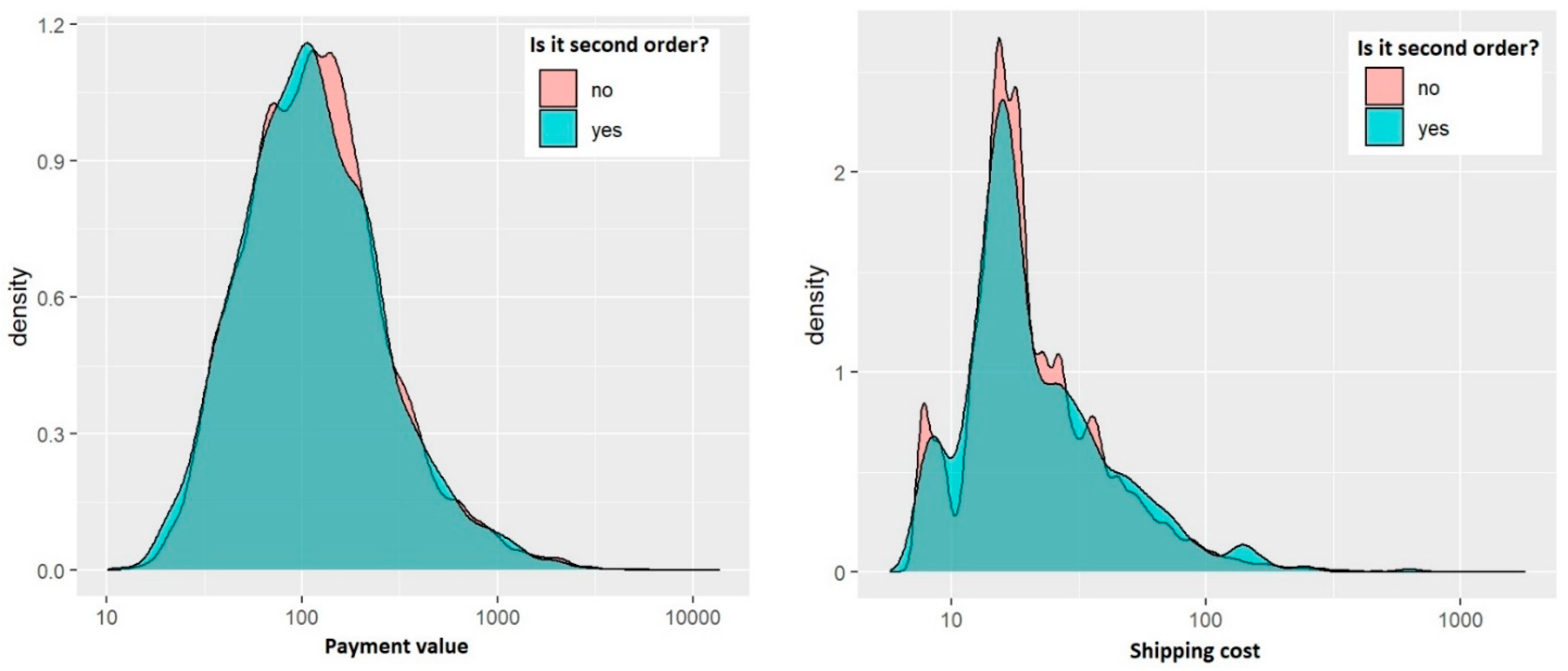
  • payment value—the value of the order in Brazilian Reals.
  • transportation value.
  • number of items the customer purchased in a particular order.
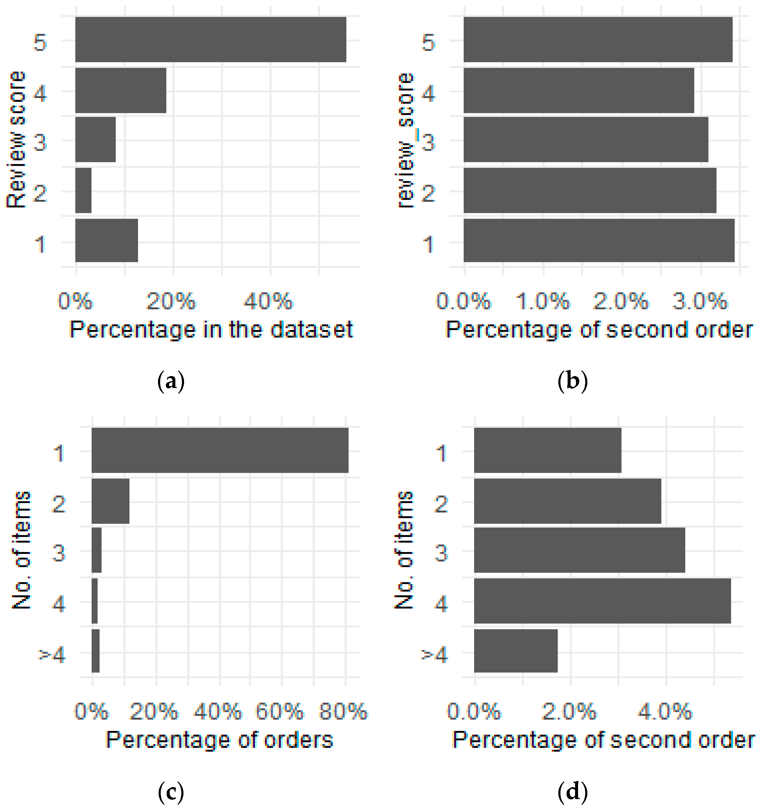
  • review of the order—the customer is able to review the finalised order in two forms: on a numerical scale of 1–5 or through a textual review. In the dataset codebook, the authors stated that not all customers wrote reviews, but this dataset was sampled so that the records without a numerical score from 1–5 were excluded. Only 50% of the records contained textual reviews. The data with a numerical review score from 1–5 was included in the models without pre-processing, but the textual reviews were pre-processed.
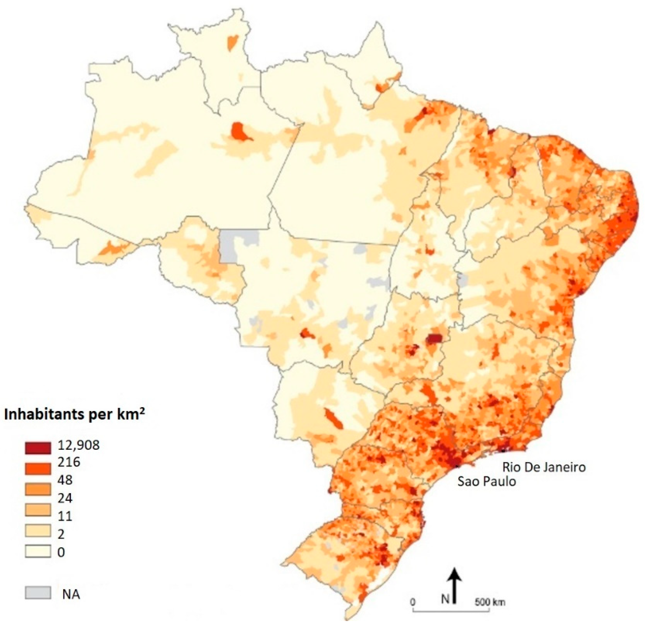
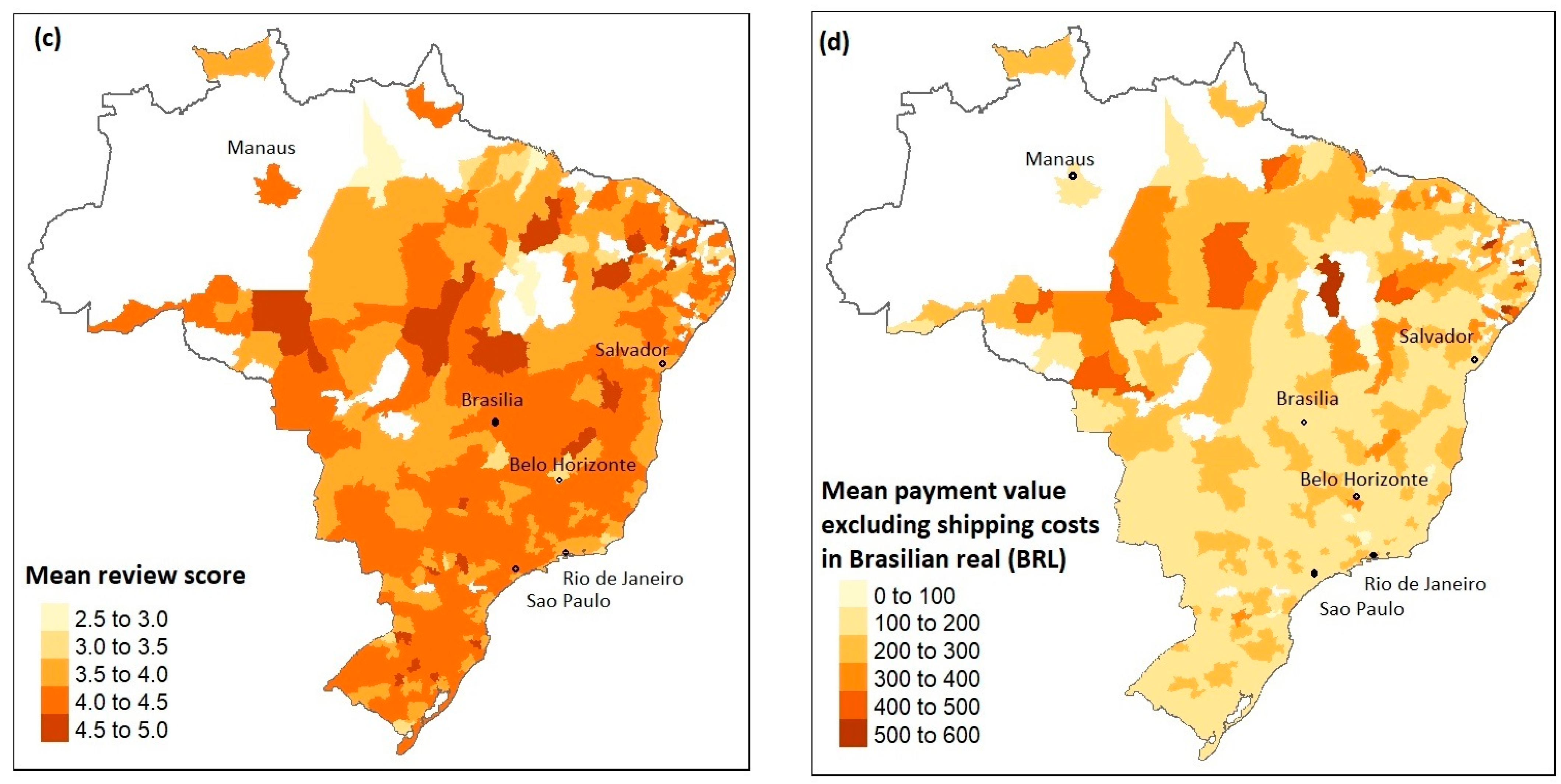
  • location of the customer—the main table containing customer information contains the 5-digit ZIP code of the customer’s home. The company also provided a mapping table in which each ZIP code is assigned to multiple latitude/longitude coordinates. This was probably done for anonymisation—so that one cannot connect the customer from the dataset with their exact house location. To obtain an exact one-to-one customer-geolocation mapping to each zip code, the most central geolocation from the mapping table was assigned. To get the most central point, the Partitioning Around Medoids (PAM) algorithm was used with only one cluster, and the algorithm was run separately for each ZIP code.
  • products bought—the dataset contains information about how many items there were in the package, as well as the product category of each item in the form of raw text. In total, there were 74 categories, but the top 15 accounted for 80% of all the purchases. To limit the number of variables used in the modelling process, the label of all the least popular categories was changed to “others”.
This study aimed to predict the likelihood of a customer becoming a repeat purchaser after just one purchase. In total, 96.6% (96,180) of the transactions in the dataset came from customers who had never previously purchased from that shop.
The geodemographic dataset was obtained from the Instituto Brasileiro de Geografia e Estatística web service. In this study, we used the 2010 census data. The dataset is divided into 558 micro-regions (a Brazilian administrative unit, similar to NUTS 3 European classification). In particular, the following 36 variables were chosen from the dataset:
  • total population of the micro-region: one variable.
  • age structure—the percentage of people in a specific age group (where the width of the groups are equal to 5 years): 20 variables.
  • percentage of people living in rural areas and urban areas: two variables.
  • percentage of immigrants compared to total micro-region population: one variable.
  • earnings structure—share of the people who earn between x0*minimum_wage and x1*minimum_wage: 11 variables.

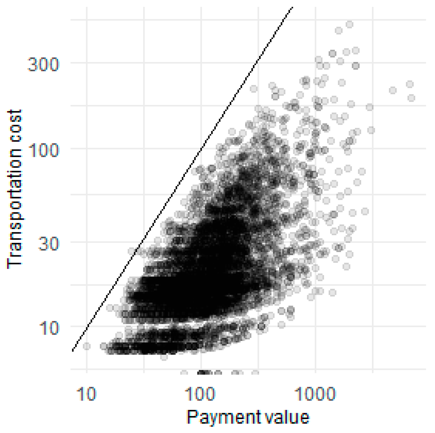
4.1. Statistics of Transactions

In the whole dataset, 96,000 orders (96.57%) were customers’ first orders (Table 1). The number of orders per customer then fell abruptly, and there were only 47 orders (0.05%) in the dataset which came from purchasers who ordered five or more times. The mean value of the transaction does not change significantly with the number of orders. If the company was successful in ensuring that the customer placed a second order, they gained about the same revenue as from the customer’s first order. In the last column, the percentages of stage-to-stage movement are presented. For example, the probability that customers who bought one time will also buy a second time was 3.18%. The same value, but from second to third order, was 8.56%. This means that encouraging the customer to buy for the second time is the hardest task the company faces. With the following purchases, the customers become more and more loyal. For this reason, in this study, only the first customer’s purchase is analysed.
The comparison of payments (left) and transport costs (right) between the groups of first-time and “loyal” customers (first and second purchase) shows that those distributions are very similar and almost overlap (Figure 4). We used the Kernel Density Estimation technique to obtain the smoothed density plots. As the distribution is highly right-skewed, we took the logarithm of the values. This means that the payment value and shipping cost would probably not be good predictors of churn in a univariate approach, although they can interact with other features and begin to have predictive power. Machine learning methods can infer such interaction by themselves. Any studies on what features should interact with payment value to improve the model’s performance are missing from the literature.
Interestingly, the values of the ordered products and the transportation cost are correlated (with Pearson correlation around 0.504). For each order value, the shipping fee was rarely bigger than the product’s value. The relationship of these values (in logarithms) with a 45° line is shown in Figure 5. This probably comes from the company’s policy to limit the transportation cost, as the customers would not buy the company’s products if the transportation costs more than the product itself.
The structure of review ratings for the whole dataset and the second purchase is somewhat surprising (Figure 6). In general, most reviews are positive—75% of the reviews score four and five, but the tendency for negative score polarisation exists, where customers unsatisfied with an order are more likely to score one than two (Figure 6a). In the context of churn, the customers who give a one-star review for the first purchase are equally likely as those who score five to make a second order. The difference in the likelihood of re-purchase between the groups is very small, ranging from 2.9% for a review that scores four (the smallest percentage) and 3.45% for a review that scores one (Figure 6b). This is unintuitive, as one would expect that clients unsatisfied with the first purchase would never buy from the same store again. It can be questioned whether these results are caused by chance and whether the review score does not influence the probability to come back at all. In particular, the difference between the percentages for scores one and five (0.003%) is so small that it is most likely caused by chance. However, the number of items purchased has predictive power for the next purchase. The more items the customer buys in the first order, the more likely it is that they will place a second order (Figure 6d). This relationship is very strong, and the re-purchase chance doubles with every item, up to four items. The re-purchase chance when buying more than four items (>4) forms a marginal amount of the overall transactions and is beyond the analysis considered here.
In the analysed case, the most popular category, “bed, bath and tables”, accounted for almost 12% of all items bought from the shop (Table 2). The statistics are sorted by the percentage of customers who made their first purchase in a specific category and later decided to buy from the shop for a second time. The differences between the probabilities of a second-purchase chance are visible—for “the best” category, the probability is 13.8%, while for the worst, it is only 1.3%. This is a promising result, and hints that the dummy variable indicating product category can serve as an important feature in the modelling phase.

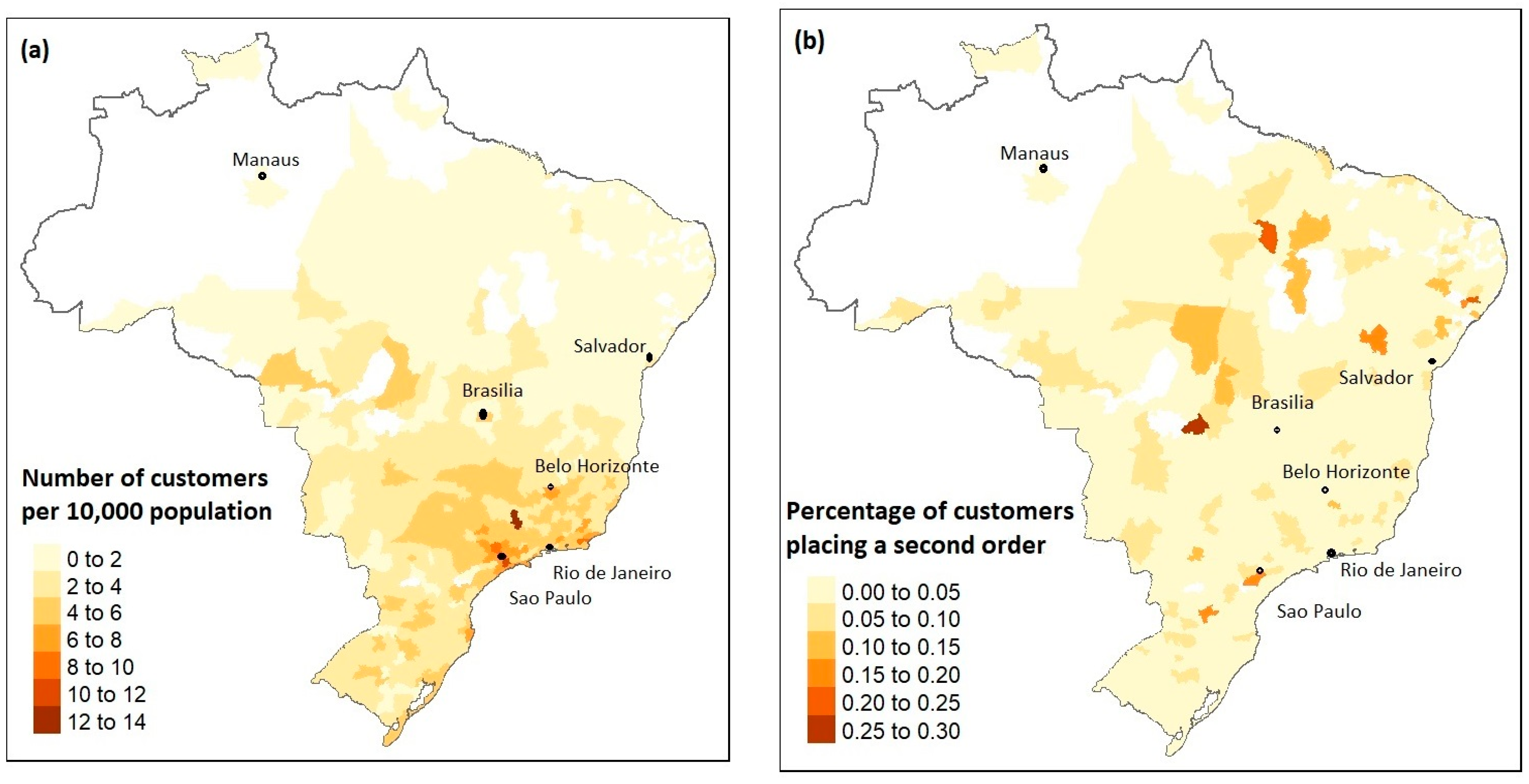
4.2. Spatial Analysis of Data

Below we compare the spatial densities of the Brazilian population (Figure 7) and Olist customers (Figure 8), which are correlated significantly (Pearson coef. ≈ 93%). The most densely populated areas are located in the southern part of the country, where the biggest cities like São Paulo and Rio de Janeiro are located (Figure 7). Another populated area is on the eastern coast. The north-western part of the country is the least populated. The distribution of customers follows this density very closely. In Figure 8, customers are shown to be aggregated to the micro-region level. Due to reliability issues, micro-regions with less than 5 customers were removed. The highest number of Olist customers per 10,000 inhabitants (Figure 8a) appears in the southern part of the country, concentrated in the triangle between the São Paulo, Rio de Janeiro and Belo Horizonte agglomerations. The percentage of second-order customers appears mainly in the northern part of the country, although this relationship is weak. The same pattern appears for the mean review score (Figure 8c). The mean transaction value (Figure 8d) is larger in the north, which is a more desolate part of Brazil (because of the Amazon Rainforest). One explanation could be that in these parts the delivery of packages is more complicated, expensive and takes more time, and thus customers are more eager to place one bigger order than multiple smaller orders. Another possibility is that in the northern part of the country, the competition between e-commerce sites is smaller, and thus customers are pushed to buy more items from one supplier.

5. Modelling Results

5.1. Results of the Pre-Modelling Phase

Topic modelling was used to extract meaningful information from the customer’s text reviews. The resulting topic assignments should help us to validate if customer perception is important for their propensity to churn. Moreover, such data can be used in other parts of CRM, such as live monitoring of customer satisfaction. The topics obtained from LDA, Gibbs Sampling and aspect extraction methods were manually assessed. In LDA and Gibbs Sampling, the topic assignments were not coherent, and the models were not able to infer topics meaningfully. The only reasonable output was produced by the last method, attention-based aspect extraction. For some of the inferred topics, all the reviews had similar content—for example, one topic included reviews which praised fast delivery (“On-time delivery”), and another contained short positive messages about the purchase (“OK”). An interesting remark is that “spam” reviews (e.g., “vbvbsgfbsbfs”, “Ksksksk”) were also classified into one topic. This suggests that topics are correctly inferred by the aspect extraction method, and the variables indicating topic assignments can improve the machine learning model. The topic modelling results with examples of reviews for each topic and proposals of topic labels are presented in Appendix B. Technically, attention-based aspect extraction was superior to latent Dirichlet allocation and its improved version and can probably discover topics better in the case of short texts. Nevertheless, using LDA is considerably easier, as this method is widely popular with a good coverage of documentation and easy-to-apply implementations. On the other hand, aspect extraction requires some level of expertise regarding neural network modelling. The available implementation requires some changes to the code so that it works on a dataset other than the one used in the original study. Besides that, neural network model training takes a couple of hours, while for LDA it takes only twenty minutes.
Customer density, obtained with the DBSCAN algorithm, divided customers into groups living in rural (sparsely populated) or urban (densely populated) areas. This information was then included in the machine learning model to test if customers from rural areas are less prone to churn. Visual inspection the assignment of customers to DBSCAN density clusters showed that the boundaries of the clusters overlapped with the boundaries of bigger cities, which proves that the clustering inferred densely populated areas correctly.
PCA-dimension reduction was applied to 36 geodemographic features to reduce the number of features that the models would have to learn, while retaining most of the information from the original set of features. The first 10 most informative PCA eigenvectors (loadings) accounted for 97.3% of the explained variance. Such a high value of explained variance means that applying the PCA transformation was successful in data compression and information preservation. Consequently, the first 10 eigenvectors (instead of 36 features) were included as explanatory variables in the modelling phase, which greatly reduced the model complexity and training time.

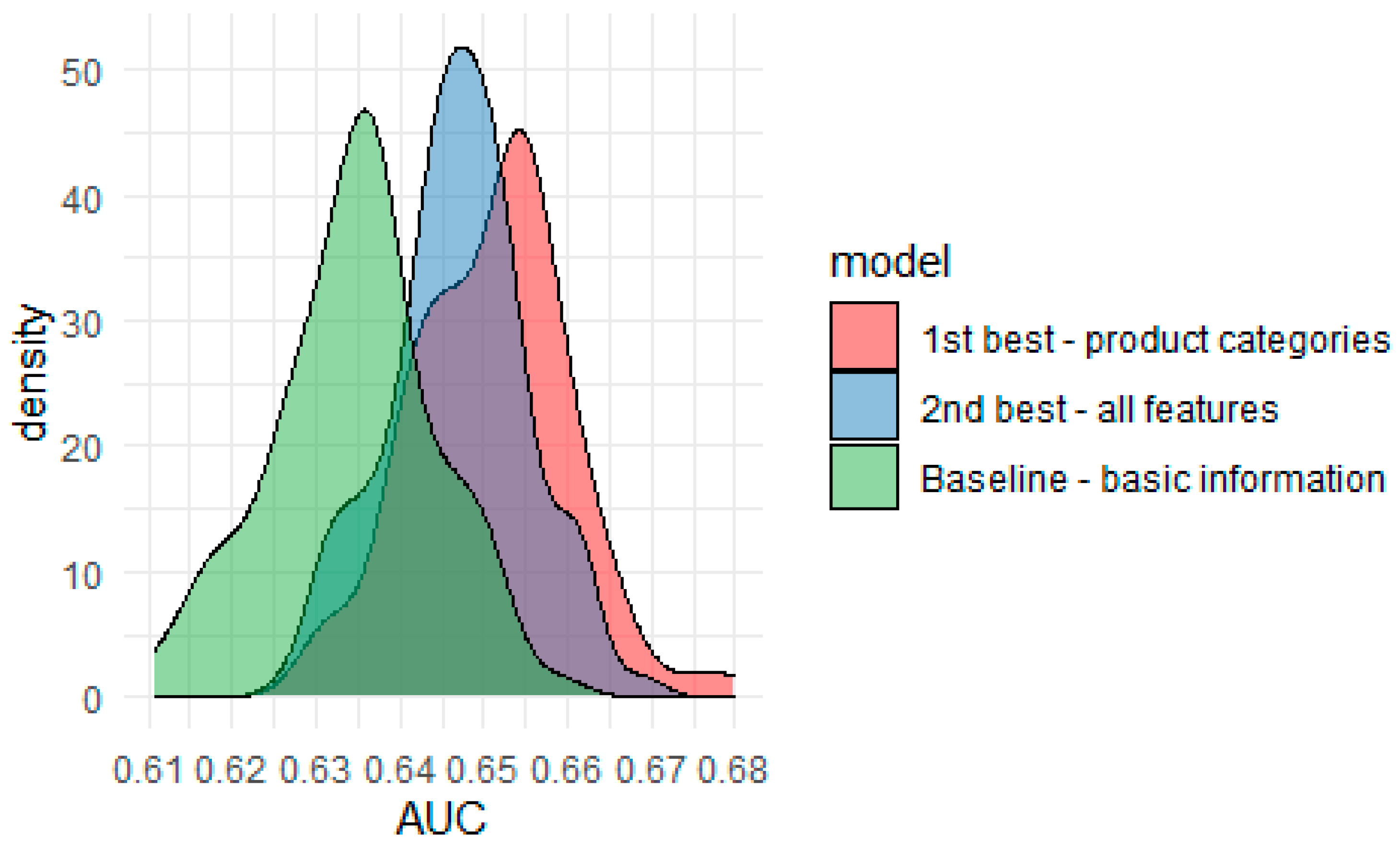
5.2. Performance Analysis

AUC metric analysis was used to compare all XGBoost and LR models tested in this study, which differed in terms of the sets of independent variables used (Table 3). All models used the same dependent variable, which was an indicator of whether the customer had placed a second order. The best AUC score in the test set was achieved by the XGBoost model with basic features combined with dummies which indicated the product categories that the customer bought during their first purchase. Its AUC was greater than 0.5, which means that the model has a predictive power better than random guessing. The second best XGB model contains all variables, with PCA-transformed demographic variables and product categories; thus, similar performance is not surprising. The percentage drop in AUC between the first and second XGB model is very small (0.6%). The model with only basic information is about 2.5% worse. The AUC score of the model based on Boruta-selected features is 0.646% less than the model, including all variables. This means that using the Boruta algorithm did not bring additional predictive power to the model. The model with review topics performed better than without them, making review topics relevant to model performance. In the case of the Logistic Regression (LR) models, the main finding is that even the best LR model (containing product categories and basic features) performed worse than the worst XGBoost model (0.586 vs. 0.625, respectively), and the ranking of models changed. This suggests that linear modelling is, in general, very poorly suited for this prediction task. AUC values for the LR model test set oscillate below 0.6, which means that the models are very poorly fitted to the data. The worst LR model (AUC test = 0.546), with the agglomeration (population) feature only, shows performance very close to the random classifier (AUC test = 0.5), so one could argue that this model does not have any predictive power. Interestingly, based on AUC values, both the LR and XGBoost models use the same features fir the highest-performing models—namely product categories and all variables. This suggests that these variables provide the biggest predictive power, regardless of the model used. The second interesting remark comes from comparing the models based on an agglomeration set of features (population density indicator). In the XGBoost model, this feature is rated as the third most informative (after excluding the Boruta set to compare meaningfully with the LR table), while it is scored as the least informative in the case of LR. One possible explanation is the inherent ability of XGBoost to create interactions between variables, while these interactions need to be included in LR models manually.
From a CRM perspective, the most important result of the modelling procedure is that the created models have predictive power for churn prediction. This means that by using the model’s predictions, a firm can forecast which customers are most likely to place a second order and can be encouraged further; and on the other hand, which customers have a very low probability of buying and whom the company should restrain from targeting to save money.
The AUC scores in Table 3 are the point estimates. One cannot guess if the performance would still be the same for a slightly different test set from such information. This is especially crucial in the case of this study, as the differences between all the XGBoost models are not large. A standard way to compare the models’ performance more robustly is using a bootstrapping technique. Observations from the test set were sampled with replacement (100 re-sample rounds), and the AUC measure was calculated with the density function. This again provided a ranking of the models (Figure 9) demonstrating that the best model used product categories and basic information, the second best used all variables, and the baseline used only basic information. The curve for the model with basic features stands out from the others. However, the difference between the highest- and second highest-performing models is not as clear—it looks like the better model has a slightly better density curve shape, but this should be investigated more thoroughly. With the Kolmogorov-Smirnov (K-S) test, we checked whether the empirical distributions came from the same probability distribution. This is a non-parametric test to assess whether two empirical samples come from the same distribution. The K-S statistic is calculated based on the largest distance between the empirical distribution functions of both samples, and this statistic is then compared against the Kolmogorov distribution. The null hypothesis in this test is that two samples come from the same underlying distribution. The test was run twice using two alternative hypotheses. The first one with H1: auc_best =/= auc_2nd_best, and the second one: H1: auc_best > auc_2nd_best. The p-value for the first hypothesis was 0.0014, which suggests that models are distinguishable. The p-value for the second hypothesis was 0.0007, which confirms that the performance of the first model (only product categories) is significantly better than that of the second one (all variables).
Aside from the statistical justification for choosing the smaller model (with fewer variables), the theory of Occam’s razor heuristic is relevant. The model with product categories has 21 variables, while the one with all variables includes 47. If there is no important reason for why the more complex approach should be used, the simpler method is usually preferable. In this case, using a simpler model has the following advantages for usage in a CRM context. First, it provides faster inference about new customers—especially in an online prediction setting when predictions must be made on the fly. Secondly, the projections are easier to interpret, and thirdly, it is easier to train and re-train the model.
Lift metric analysis computes the likelihood of re-purchase in ranked groups of customers. More specifically, one creates a ranking of customers in which they are sorted by their likelihood to buy for a second time. For each cumulative group in the ranking (the top 1% of customers, the top 10%, etc.), one can compute which percentage of this group is truly buying for the second time. An ultimate goal of customer churn prediction is gaining information on which customers are most likely to place a second order. Lift metric analysis is a go-to tool for measuring the performance of targeting campaigns. It is also very easily understood by CRM experts without a deep knowledge of statistics and machine learning.
Technically, in lift metric analysis, customers are divided into segments defined as the top x% of the ranking which is output by the targeting model. The procedure for calculating the lift metric, for example, of the top 5% of customers, is defined as follows:
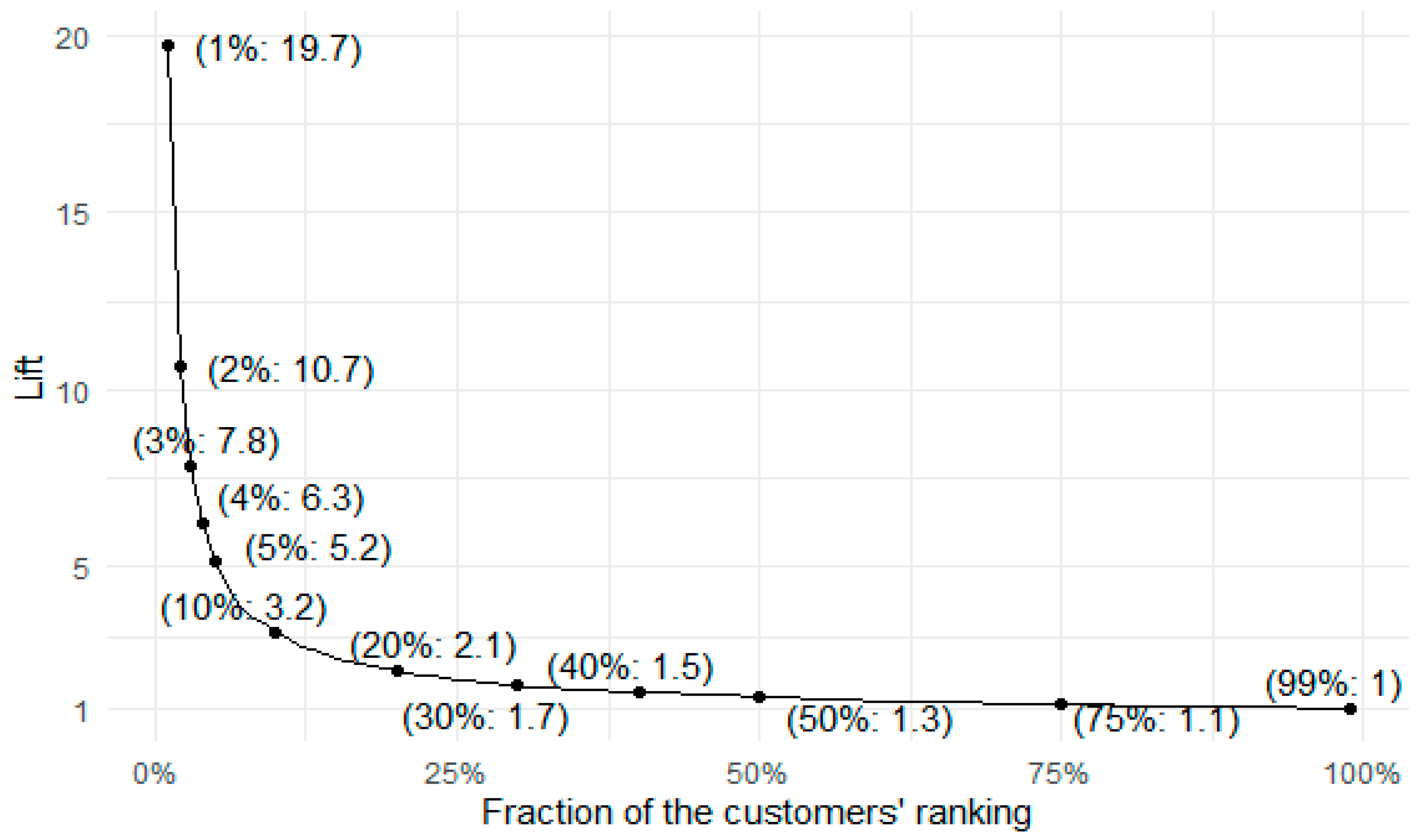
  • Sample 5% of all customers. Calculate the share of these customers (share_random), who have a positive response (who truly bought for a second time).
  • Using a machine learning model, predict the probability of buying for a second time all the customers. Then, rank these customers by the likelihood and select the top 5% with the highest probability. Calculate the share of these customers (share_model) who have a positive response.
  • Calculate the lift measure as share_model/share_random. If the lift value is equal to one, this means that the machine learning model is no better at predicting the top 5% of the best customers than random guessing. The bigger the value, the better the model is in the case of this top 5% segment. For example, if the lift metric is equal to three, the model is three times better at targeting promising customers than random targeting.
Such calculations can be repeated for multiple customer segments, typically defined by the top x% of the ranking. CRM experts can then consider lift values for various segments, combine this insight with targeting cost, and decide what percentage of the customers should be targeted.
A lift curve (Figure 10, Appendix C) is convenient for visualising lift metrics for multiple segments at once, with a fraction of top customers ranked by probability to re-purchase on the x-axis and lift value on the y-axis. The shape of the plot resembles the 1/x function. The lift values are very big for the smallest percentage of the best customers to target, and they get smaller quickly. This means that the more customers the company would like to target based on the model’s prediction, the less marginal the effects would be from using the model. For example, for the top 1% of customers, the model can predict retention 18.7 times better than a random targeting approach. It is still very effective for the top 5%, being 4.2 times better than random. If one wants to target half of the customers, the improvement over random targeting is 0.3 (130%), and although this value is less impressive than for smaller percentages, it is still an improvement over random targeting.

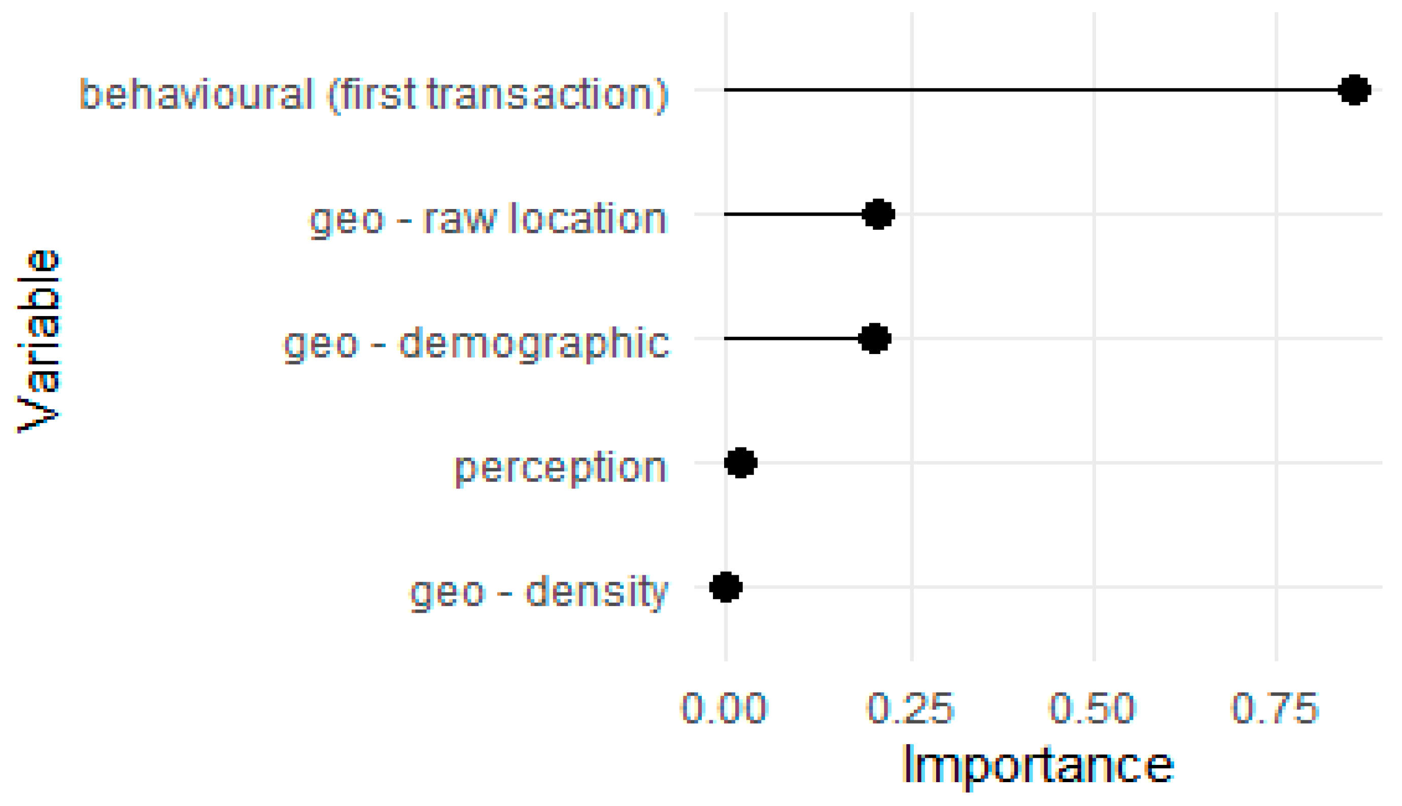
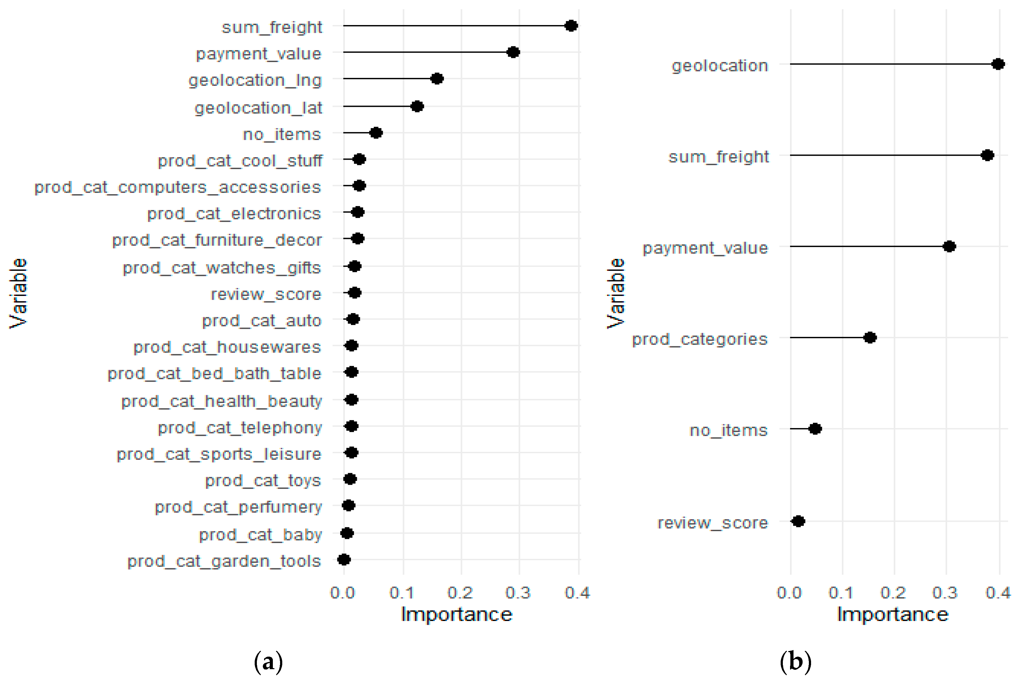
5.3. Understanding Feature Impact with Explainable Artificial Intelligence

Discovering which features to use and how to drive the predictions of customer churn/loyalty is very important for successful CRM. In this study, permutation-based variable importance is first employed to check if particular sets of features have any influence on the model’s predictions, and if they do, how strong this influence is. Secondly, the partial dependence profile technique is used to check the direction of this influence.
Permutation-based Variable Importance (VI) was assessed for the two best XGBoost models (with all variables and with basic features and product categories). VI can answer questions about the impact of particular sets of variables. The variables were grouped into five sets:
  • behavioural—variables describing the first transaction of the customer: payment value, product category, etc.
  • perception—variables describing quantitative revives (on a scale of 1–5) and dummies for textual (topic) reviews.
  • “geo” variables—with three subgroups:
    demographic variables describing the population structure of a customer’s region.
    raw location, being simply longitude/latitude coordinates.
    density variable, indicating whether the customer lives in a densely populated area.
Considering all variables in the five thematic groups (Figure 11), the best set of variables contains the behavioural features. The following two sets, geo-demographic and raw spatial location, have a similar moderate influence. The perception variables (reviews) and the density population (rural/urban) indicator have the lowest impact on the model’s predictions. These results follow our expectations. We show that a customers’ propensity to churn depends on: (i) payment value for the first order, number of items bought, shipping cost, (ii) categories of the products bought, (iii) demographic environment of the customer and (iv) customer location. At the same time, the customers’ propensity to churn is not influenced by: (i) population density in the customer’s area and division into rural and urban areas, (ii) quantitative review of the first purchase or (iii) qualitative review summarised as a topic.
The second best XGB model which includes all variables reveals the detailed impact 1080 of all considered factors, individually (Figure 12a) and in groups (Figure 12b). The most important variables are the transportation cost, the value paid, and the geo-location provided by longitude and latitude. Most of the dummies which indicate product categories are in the latter part of the ranking. One can question why these features are ranked as relatively unimportant variables when they lead to a 2.5% gain in AUC compared to the model which does not used these features. This is because conceptually, all dummies which indicate product category are considered separately. The same effect is seen with geographic coordinates. To account for this, feature importance for these variable sets (“geolocation” and “prod_categories”) was used instead of individual feature importance. This information is presented in the right subfigure. After this operation, product categories gained relative importance to become the fourth most important variable, and the geolocation variable set becomes more important than payment value and transportation cost.
Partial Dependence Profile (PDP) (Figure 13) allows for testing the direction and strength of the influence of various factors on customer churn. It was applied to payment value for the first order, the number of items purchased, customer location and review score. The PDP for payment value (Figure 13a) is non-monotonous. From an analysis of the smoothed model response (blue line), one can say that it continuous to increase until the point of around 100. This means that on average, until the payment value reaches 100, the bigger the payment value, the bigger probability of placing a second order by the customer as predicted by the model. After this threshold of 100, the probability of buying for the second time falls slowly. The PDP for the number of items purchased (Figure 13b) shows that the relationship between the number of items bought in the first purchase and the probability of the second purchase is negative—the more items purchased, the less likely the second purchase. One must remember that there is only one product in 80% of the orders, while in 10% there are two items. At the same time, the drop in the model’s response between one and two items is not very abrupt, meaning that this feature on its own cannot serve as a very good discriminator of customer churn for most of the observations. For CRM, information about such a relationship can lead to the following trade-off. The more the customer buys in the first purchase, the bigger the chance that they will not make a second purchase. This can have implications in cross-selling campaigns. The company can maximise the revenue from the first transaction by making the customer buy more, but then there is a bigger possibility that the customer will not make the second purchase. In the case of the PDP for geolocation data (Figure 13c), the predictions are the highest in two distinct areas—one having its centre close to Brasilia (the new capital of the country) and the other one on the same latitude but closer to the western country border. The predictions form a visible pattern in stripes, which comes from a limitation of the model underlying the XGBoost method: decision trees [69]. A simple decision tree algorithm works by partitioning the feature space on a discrete basis. A typical output of such a model in 2D space is the formation of visible rectangles. Because XGBoost consists of stacked decision trees, the resulting partition pattern is a bit more complex, but decision-tree-typical artefacts are still visible. The PDP for review scores (Figure 13d) should be treated with caution, as variable importance assessment showed it to be relatively non-important, and the model response is relatively flat in reaction to changes in review score. For reviews which score one and two, the response does not change at all, meaning that it does not matter “how bad” the review is. Rather, it shows that unsatisfied customers will not buy again in general. With scores which range from two to five, the model response increases monotonically as is expected.

6. Discussion, Implications and Conclusions

This study aimed to build and test a comprehensive churn model for e-commerce using a transactions dataset from the Brazilian Olist e-commerce retail company. The study is not typical as customers were not bound by contract, their loyalty rate was very low (one digit, ca. 3.3%) and churn was predicted without long purchase history but by using the first transaction only. Those challenges have been met by enriching the transactional database (including typical behavioural data on the purchase value, shipping cost, product categories and number of items in the first purchase) by analysing customer location (zip-code) and their socio-economic environment (as geodemographic data for the customer’s region from census, rural/urban location of the customer) and perception features provided as score and text reviews by the customer.
Results of the study are essential for CRM development. As expected from other studies, behavioural features, including the category of the product purchased (analysed as category dummies from one-hot encode), payment value and shipping cost are important and significant for loyalty prediction as in [3,9,21,39]. We found that customers buying one or two items are more likely to make a second purchase than the customers who bought three or more items. Geodemographic features describing population structure in a customer’s region as in [16,19] and regional location of the customer and geographical factors as in [3,19,43,70] (analysed as raw geo-coordinates lat/long from zip code) also play a role in predicting loyalty. Local population density, classifying areas with DBSCAN into rural or urban, had little importance in churn modelling. However, we found that textual information does not always add value to the model as in [71,72]. We have shown that the popular Latent Dirichlet Allocation method, a go-to model for topic modelling, did not yield meaningful results as the reviews were too short and the neural-network-based aspect extraction method performed much better. However, even when inferring the topic was successful, it was shown that this feature was not important for predicting customer churn. For modelling, we used two algorithms. Machine learning Extreme Gradient Boosting (XGBoost) performed significantly better than logistic regression, mostly in computation time and prediction quality, showing the same direction and strength of explanatory variables. The power of machine learning other than the p-value approach to detect important factors lies in primarily using novel solutions such as permutation-based variable importance, bootstrapped AUC scores or partial dependence profile, all being a part of XAI solutions (explainable artificial intelligence). However, when important relationships are discovered, the logistic regression model built on guidelines from ML may also be efficient, while its inherent explainability is its advantage.
Managerial implications from this study are straightforward. CRM, especially targeted towards churn prediction, is challenging but feasible, even with no-history data. Transaction, location and geodemographic data are the most relevant predictors of customer churn, and they should be considered first. Product categories purchased in the first transaction may influence the propensity to churn positively or negatively—this is to be analysed carefully in further studies. That means that besides behavioural and transactional variables (which do not require much resource investment for pre-processing), the best variables came from census data and included spatial dimensions. Companies should consider including spatial analyses of the customer as a standard. On the contrary, customer perception proxied by the numeric reviews and the topics of the text reviews were shown to be not important—according to our experience, text processing is a costly procedure with inferior results. The predictions obtained from the model can be used in customer targeting to address particular actions to the customers who are most likely to stay with the company. However, to successfully integrate the model with the company’s data environment, many more issues have to be addressed. This includes (i) writing input data validation, (ii) setting up the server to host the model so that it can make predictions for new and incoming customers, and (iii) creating a continuous evaluation system so that the performance of the model can be monitored and checked to ensure it does not deteriorate over time.
There are some limitations of this study. The first one is technical—only two algorithms were tested. The reason for not including more models was resource constraints; the training of all the models used in this study took around 30 h. Performing model training and validation is easily parallelisable, so a potential improvement would be using multi-CPU cloud infrastructure to test more models in a shorter time. The second one refers to problems with possible comparisons. Previous studies often used data from stationery shops and/or where customers were bound with contract relations, which may affect the importance of the factors considered. Many other studies also reported model quality rather than the impact of the variables. The presented analysis is also pioneering in its approach and filling of the research gaps, making it partly incomparable to previous studies and opening new paths for further examination. The third limitation results from the dataset which was used in this study. The analysed transactions were made in 2016–2018 and, therefore, were pre-COVID-19. One can expect that during the COVID-19 pandemic, e-commerce has been driven by other factors and different customer behaviour than in pre- and post-pandemic times. This also opens the path for further research and comparative studies to understand whether the listed factors are universal and independent of circumstance.
The above listed limitations establish research prospects, future directions and recommendations. Except for a need for post-COVID comparisons, there is a wide gap in churn studies using geographical and spatial information. Validation of presented results should use the proposed methodology as well as the other tools such as spatial autocorrelation analysis, geographically weighted regression, spatial classification, Euclidean distance fields technique [69], etc. In general, spatial methods are based on the assumption that spatially close customers tend to have similar behaviour and characteristics. Additionally, as this study is pioneering in merging minor loyalty rate, first-purchase data only, non-contract customer relations, spatial factors and textual reviews, the prospective studies should validate this approach on other case studies.

Author Contributions

Conceptualisation, K.M. and K.K.; methodology, K.M.; software, K.M.; validation, K.M. and K.K.; formal analysis, K.M.; investigation, K.M.; resources, K.M.; data curation, K.M.; writing—original draft preparation, K.M.; writing—review and editing, K.K.; visualisation, K.M..; supervision, K.K.; project administration, K.K.; funding acquisition, K.K. All authors have read and agreed to the published version of the manuscript.

Funding

This research received no external funding.

Institutional Review Board Statement

Not applicable.

Informed Consent Statement

Not applicable.

Data Availability Statement

Data used in the research are publicly available, originally at https://www.kaggle.com/olistbr/brazilian-ecommerce (accessed on 15 September 2021) and https://sidra.ibge.gov.br/tabela/3548 (accessed on 15 September 2021). Pre-processed data are available at https://app.sugarsync.com/iris/wf/D1836703_09668593_7630608 (accessed on 15 September 2021).

Conflicts of Interest

The authors declare no conflict of interest.

Appendix A

Joining the data from the Brazilian census and the e-commerce company sources proved to be challenging. There were multiple reasons for this:
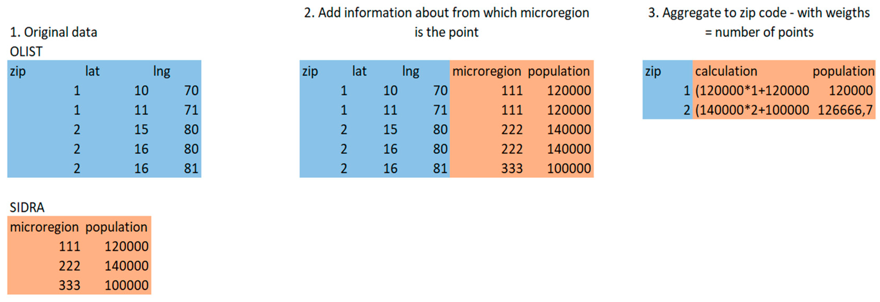
  • In the e-commerce dataset, the spatial dimensions are encoded mainly in the form of ZIP codes, while in the demographic dataset they are in the form of micro-regions (a Brazilian administrative unit).
  • The boundaries of zip codes and micro-regions do not align.
  • The customer’s geolocation data has three columns—zip code and lat/long coordinates. For each zip code, there are multiple entries for coordinates. This probably means that the company has exact coordinates of each of their customers but decided to not provide exact customer-location mapping in the public dataset for anonymisation reasons. Because of this, the boundaries of zip codes cannot be specified precisely, and one has to rely on the particular points from this zip code area.
An approach presented in a paper in response to the challenge of joining these two data sources was as follows:
  • For each point in the geolocation dataset, establish in which micro-region it is located, then join the dataset for that region to the OLIST geolocation dataset.
  • Group the dataset by zip code and calculate the mean of each of the features in the dataset; in this case, this mean would be a weighted mean (weighted in the form of “how many customers are in this area?”) (An example is shown in Figure A1).
Figure A1. Diagram depicting spatial join of transaction and demographic databases.
Jtaer 17 00009 g0a1

Appendix B

Table A1. Topics inferred by attention-based aspect extraction.
Topic No.Topic DescriptionNumber of ReviewsPercent of Customers with Second OrderExample Review
0Mentions product97203.2%Reliable seller, ok product and delivery before the deadline.
great seller arrived before the deadline, I loved the product
Very good quality product, arrived before the promised deadline
1Unsatisfied (mostly about delivery)14392.8%I WOULD LIKE TO KNOW WHAT HAS BEEN, I ALWAYS RECEIVED AND THIS PURCHASE NOW HAS DISCUSSED
Terrible
I would like to know when my product will arrive? Since the delivery date has passed, I would like an answer, I am waiting!
2Short positive message22703.6%Store note 10
OK I RECOMMEND
OK
3Short positive message, but about the product only13792.9%Excellent quality product
Excellent product.
very good, I recommend the product.
4Non-coherent topic63393.6%I got exactly what I expected. Other orders from other sellers were delayed, but this one arrived on time.
I bought the watch, unisex and sent a women's watch, much smaller than the specifications of the ad.
so far I haven't received the product.
5Positive message but longer than topic 211944.5%Wonderful
super recommend the product which is very good!
Everything as advertised.... Great product...
6Problems with delivery—wrong products, too many/too little things in package28923.8%I bought two units and only received one and now what do I do?
I bought three packs of five sheets each of transfer paper for dark tissue and received only two
The delivery was split in two. There was no statement from the store. I came to think that they had only shipped part of the product.
7Good comments about particular seller48393.4%Congratulations lannister stores loved shopping online safe and practical Congratulations to all happy Easter
I recommend the seller...
congratulations station... always arrives with a lot of antecedence.. Thank you very much....
8Short message, mostly about quality of the product38083.4%But a little, braking... for the value ta Boa.
Very good. very fragrant.
I loved it, beautiful, very delicate
9non-coherent12753.4%The purchase was made easily. The delivery was made well before the given deadline. The product has already started to be used and to date, without problems.
I hope it lasts because it is made of fur.
I asked for a refund and no response so far
10Short message, lots of times wrong spelling/random letters159.1%vbvbsgfbsbfs
I recommend... mayor;
Ksksksk
11non-coherent26142.5%I always buy over the Internet and delivery takes place before the agreed deadline, which I believe is the maximum period. At stark, the maximum term has expired and I have not yet received the product.
Great store for partnership: very fast, well packaged and quality products! Only the cost of shipping that was a little sour.
I DID NOT RECEIVE THE PRODUCT AND IS IN THE SYSTEM I RECEIVED BEYOND PAYING EXPENSIVE SHIPPING
12Praises about the product20032.2%very beautiful and cheap watch.
Good product, but what came to me does not match the photo in the ad.
Beautiful watch I loved it
13Short positive message about the delivery17883.0%On-time delivery
It took too long for delivery
super fast delivery.... arrived before the date...

Appendix C. Table of Lift Values for Selected Quantiles

Table A2. Lift values for selected quantiles—general probability of buying for second time is 3.29%.
Fraction of CustomersNo. Customers in GroupProbability in Selected GroupLift
1%3200.6519.71
2%6400.3510.66
3%9590.267.84
4%12790.216.26
5%15980.175.16
10%31960.103.16
20%63920.072.07
30%95870.051.65
40%12,7830.051.48
50%15,9780.041.35

References

  1. Dick, A.S.; Basu, K. Customer Loyalty: Toward an Integrated Conceptual Framework. J. Acad. Mark. Sci. 1994, 22, 99–113. [Google Scholar] [CrossRef]
  2. Gefen, D. Customer Loyalty in e-Commerce. J. Assoc. Inf. Syst. 2002, 3, 2. [Google Scholar] [CrossRef]
  3. Buckinx, W.; Poel, D.V.D. Customer base analysis: Partial defection of behaviourally loyal clients in a non-contractual FMCG retail setting. Eur. J. Oper. Res. 2005, 164, 252–268. [Google Scholar] [CrossRef]
  4. Bach, M.P.; Pivar, J.; Jaković, B. Churn Management in Telecommunications: Hybrid Approach Using Cluster Analysis and Decision Trees. J. Risk Financ. Manag. 2021, 14, 544. [Google Scholar] [CrossRef]
  5. Nie, G.; Rowe, W.; Zhang, L.; Tian, Y.; Shi, Y. Credit Card Churn Forecasting by Logistic Regression and Decision Tree. Expert Syst. Appl. 2011, 38, 15273–15285. [Google Scholar] [CrossRef]
  6. Dalvi, P.K.; Khandge, S.K.; Deomore, A.; Bankar, A.; Kanade, V.A. Analysis of customer churn prediction in telecom industry using decision trees and logistic regression. In Proceedings of the 2016 Symposium on Colossal Data Analysis and Networking (CDAN), Indore, India, 18–19 March 2016; pp. 1–4. [Google Scholar]
  7. Gregory, B. Predicting Customer Churn: Extreme Gradient Boosting with Temporal Data. arXiv 2018, arXiv:1802.03396. [Google Scholar]
  8. Xiao, J.; Jiang, X.; He, C.; Teng, G. Churn prediction in customer relationship management via GMDH-based multiple classifiers ensemble. IEEE Intell. Syst. 2016, 31, 37–44. [Google Scholar] [CrossRef]
  9. Miguéis, V.; Van Den Poel, D.; Camanho, A.; e Cunha, J.F. Modeling partial customer churn: On the value of first product-category purchase sequences. Expert Syst. Appl. 2012, 39, 11250–11256. [Google Scholar] [CrossRef]
  10. Tamaddoni Jahromi, A.; Sepehri, M.M.; Teimourpour, B.; Choobdar, S. Modeling Customer Churn in a Non-Contractual Setting: The Case of Telecommunications Service Providers. J. Strateg. Mark. 2010, 18, 587–598. [Google Scholar] [CrossRef] [Green Version]
  11. Sithole, B.T.; Njaya, T. Regional Perspectives of the Determinants of Customer Churn Behaviour in Various Indus-tries in Asia, Latin America and Sub-Saharan Africa. Sch. J. Econ. Bus. Manag. 2018, 5, 211–217. [Google Scholar]
  12. Ngai, E.W.; Xiu, L.; Chau, D. Application of data mining techniques in customer relationship management: A literature review and classification. Expert Syst. Appl. 2009, 36, 2592–2602. [Google Scholar] [CrossRef]
  13. Hadden, J.; Tiwari, A.; Roy, R.; Ruta, D. Computer assisted customer churn management: State-of-the-art and future trends. Comput. Oper. Res. 2007, 34, 2902–2917. [Google Scholar] [CrossRef]
  14. Mozer, M.C.; Richard, W.; David, B.G.; Eric, J.; Howard, K. Predicting Sub-scriber Dissatisfaction and Improving Retention in the Wireless Telecommunications Industry. IEEE Trans. Neural Netw. 2000, 11, 690–696. [Google Scholar] [CrossRef] [Green Version]
  15. Long, H.V.; Son, L.H.; Khari, M.; Arora, K.; Chopra, S.; Kumar, R.; Le, T.; Baik, S.W. A New Approach for Construction of Geodemographic Segmentation Model and Prediction Analysis. Comput. Intell. Neurosci. 2019, 2019, 9252837. [Google Scholar] [CrossRef]
  16. Zhao, Y.; Li, B.; Li, X.; Liu, W.; Ren, S. Customer Churn Prediction Using Improved One-Class Support Vector Machine. In Proceedings of the Computer Vision–ECCV 2014; Springer: Berlin/Heidelberg, Germany, 2005; pp. 300–306. [Google Scholar]
  17. Jha, M. Understanding Rural Buyer Behaviour. IIMB Manag. Rev. 2003, 15, 89–92. [Google Scholar]
  18. Kracklauer, A.; Passenheim, O.; Seifert, D. Mutual customer approach: How industry and trade are executing collaborative customer relationship management. Int. J. Retail. Distrib. Manag. 2001, 29, 515–519. [Google Scholar] [CrossRef]
  19. De Caigny, A.; Coussement, K.; De Bock, K.W.; Lessmann, S. Incorporating textual information in customer churn prediction models based on a convolutional neural network. Int. J. Forecast. 2020, 36, 1563–1578. [Google Scholar] [CrossRef]
  20. Bardicchia, M. Digital CRM-Strategies and Emerging Trends: Building Customer Relationship in the Digital Era; Independently published; 2020. [Google Scholar]
  21. Oliveira, V.L.M. Analytical Customer Relationship Management in Retailing Supported by Data Mining Techniques. Ph.D. Thesis, Universidade do Porto, Porto, Portugal, 2012. [Google Scholar]
  22. Achrol, R.S.; Kotler, P. Marketing in the Network Economy. J. Mark. 1999, 63, 146. [Google Scholar] [CrossRef]
  23. Choi, D.H.; Chul, M.K.; Kim, S.I.; Kim, S.H. Customer Loyalty and Disloyalty in Internet Re-tail Stores: Its Antecedents and Its Effect on Customer Price Sensitivity. Int. J. Manag. 2006, 23, 925. [Google Scholar]
  24. Burez, J.; Poel, D.V.D. CRM at a pay-TV company: Using analytical models to reduce customer attrition by targeted marketing for subscription services. Expert Syst. Appl. 2007, 32, 277–288. [Google Scholar] [CrossRef] [Green Version]
  25. Au, W.-H.; Chan, K.C.; Yao, X. A novel evolutionary data mining algorithm with applications to churn prediction. IEEE Trans. Evol. Comput. 2003, 7, 532–545. [Google Scholar] [CrossRef] [Green Version]
  26. Verbeke, W.; Martens, D.; Mues, C.; Baesens, B. Building comprehensible customer churn prediction models with advanced rule induction techniques. Expert Syst. Appl. 2011, 38, 2354–2364. [Google Scholar] [CrossRef]
  27. Paruelo, J.; Tomasel, F. Prediction of Functional Characteristics of Ecosystems: A Comparison of Artificial Neural Networks and Regression Models. Ecol. Model. 1997, 98, 173–186. [Google Scholar] [CrossRef]
  28. Murthy, S.K. Automatic Construction of Decision Trees from Data: A Multi-Disciplinary Survey. Data Min. Knowl. Discov. 1998, 2, 345–389. [Google Scholar] [CrossRef]
  29. Caruana, R.; Niculescu-Mizil, A. An empirical comparison of supervised learning algorithms. In Proceedings of the 23rd International Conference on Machine Learning-ICML ’06, Pittsburgh, PA, USA, 25–29 June 2006; Association for Computing Machinery (ACM): New York, NY, USA, 2006; pp. 161–168. [Google Scholar]
  30. Chen, T.; He, T.; Benesty, M.; Khotilovich, V.; Tang, Y.; Cho, H. Xgboost: Extreme Gradient Boosting; R Package Version 0.4-2; 2015; Volume 1, pp. 1–4. [Google Scholar]
  31. Nielsen, D. Tree Boosting with Xgboost-Why Does Xgboost Win “Every” Machine Learning Competition? Master’s Thesis, Norwegian University of Science and Technology’s, Trondheim, Norway, 2016. [Google Scholar]
  32. Nanayakkara, S.; Fogarty, S.; Tremeer, M.; Ross, K.; Richards, B.; Bergmeir, C.; Xu, S.; Stub, D.; Smith, K.; Tacey, M.; et al. Characterising Risk of in-Hospital Mortality Following Cardiac Arrest Using Machine Learning: A Retrospective International Registry Study. PLoS Med. 2018, 15, e1002709. [Google Scholar] [CrossRef] [Green Version]
  33. Biecek, P.; Tomasz, B. Explanatory Model Analysis: Explore, Explain, and Examine Predictive Models; CRC Press: Boca Raton, FL, USA, 2021. [Google Scholar]
  34. Doshi-Velez, F.; Kim, B. Towards a Rigorous Science of Interpretable Machine Learning. arXiv 2017, arXiv:1702.08608. [Google Scholar]
  35. Rai, A. Explainable AI: From black box to glass box. J. Acad. Mark. Sci. 2019, 48, 137–141. [Google Scholar] [CrossRef] [Green Version]
  36. Suryadi, D. Predicting Repurchase Intention Using Textual Features of Online Customer Reviews. In Proceedings of the 2020 International Conference on Data Analytics for Business and Industry: Way Towards a Sustainable Economy (ICDABI), Sakheer, Bahrain, 26–27 October 2020; pp. 1–6. [Google Scholar] [CrossRef]
  37. Lucini, F.R.; Tonetto, L.M.; Fogliatto, F.S.; Anzanello, M.J. Text mining approach to explore dimensions of airline customer satisfaction using online customer reviews. J. Air Transp. Manag. 2020, 83, 101760. [Google Scholar] [CrossRef]
  38. Schmittlein, D.C.; Peterson, R.A. Customer Base Analysis: An Industrial Purchase Process Application. Mark. Sci. 1994, 13, 41–67. [Google Scholar] [CrossRef]
  39. Bhattacharya, C.B. When Customers Are Members: Customer Retention in Paid Membership Contexts. J. Acad. Mark. Sci. 1998, 26, 31–44. [Google Scholar] [CrossRef]
  40. Athanassopoulos, A.D. Customer Satisfaction Cues To Support Market Segmentation and Explain Switching Behavior. J. Bus. Res. 2000, 47, 191–207. [Google Scholar] [CrossRef]
  41. Lee, J.Y.; Bell, D.R. Neighborhood Social Capital and Social Learning for Experience Attributes of Products. Mark. Sci. 2013, 32, 960–976. [Google Scholar] [CrossRef] [Green Version]
  42. Verbeke, W.; Dejaeger, K.; Martens, D.; Hur, J.; Baesens, B. New insights into churn prediction in the telecommunication sector: A profit driven data mining approach. Eur. J. Oper. Res. 2012, 218, 211–229. [Google Scholar] [CrossRef]
  43. De la Llave, M.Á.; López, F.A.; Angulo, A. The Impact of Geographical Factors on Churn Pre-diction: An Application to an Insurance Company in Madrid’s Urban Area. Scand. Actuar. J. 2019, 3, 188–203. [Google Scholar] [CrossRef]
  44. Harris, R.; Sleight, P.; Webber, R. Geodemographics, GIS and Neighbourhood Targeting; John Wiley & Sons: Hoboken, NJ, USA, 2005; Volume 8. [Google Scholar]
  45. Singleton, A.D.; Spielman, S.E. The Past, Present, and Future of Geodemographic Research in the United States and United Kingdom. Prof. Geogr. 2014, 66, 558–567. [Google Scholar] [CrossRef] [Green Version]
  46. Braun, T.; Webber, R. Targeting Customers: How to Use Geodemographic and Lifestyle Data in Your Business (3rd edition). Interact. Mark. 2004, 6, 200–201. [Google Scholar] [CrossRef]
  47. Sun, T.; Wu, G. Consumption patterns of Chinese urban and rural consumers. J. Consum. Mark. 2004, 21, 245–253. [Google Scholar] [CrossRef]
  48. Sharma, S.; Singh, M. Impact of brand selection on brand loyalty with special reference to personal care products: A rural urban comparison. Int. J. Indian Cult. Bus. Manag. 2021, 22, 287. [Google Scholar] [CrossRef]
  49. Felbermayr, A.; Nanopoulos, A. The Role of Emotions for the Perceived Usefulness in Online Customer Reviews. J. Interact. Mark. 2016, 36, 60–76. [Google Scholar] [CrossRef]
  50. Zhao, Y.; Xu, X.; Wang, M. Predicting overall customer satisfaction: Big data evidence from hotel online textual reviews. Int. J. Hosp. Manag. 2019, 76, 111–121. [Google Scholar] [CrossRef]
  51. Howley, T.; Madden, M.G.; O’Connell, M.-L.; Ryder, A.G. The Effect of Principal Component Analysis on Machine Learning Accuracy with High Dimensional Spectral Data. In Proceedings of the International Conference on Innovative Techniques and Applications of Artificial Intelligence, Cambridge, UK, 15–17 December 2020; Springer: Berlin/Heidelberg, Germany, 2005. [Google Scholar]
  52. Corner, S. Choosing the Right Type of Rotation in PCA and EFA. JALT Test. Eval. SIG Newsl. 2009, 13, 20–25. [Google Scholar]
  53. Blei, D.M.; Ng, A.Y.; Jordan, M.I. Latent Dirichlet Allocation. J. Mach. Learn. Res. 2003, 3, 993–1022. [Google Scholar]
  54. Hong, L.; Davison, B.D. Empirical study of topic modeling in Twitter. In Proceedings of the First Workshop on Social Media Analytics-SOMA ’10; Association for Computing Machinery (ACM): New York, NY, USA, 2010; pp. 80–88. [Google Scholar]
  55. Yin, J.; Wang, J. A dirichlet multinomial mixture model-based approach for short text clustering. In Proceedings of the 20th ACM SIGKDD International Conference on Knowledge Discovery and Data Mining, New York, NY, USA, 24–27 August 2014; Association for Computing Machinery (ACM): New York, NY, USA, 2014; pp. 233–242. [Google Scholar] [CrossRef]
  56. Mikolov, T.; Chen, K.; Corrado, G.; Dean, J. Efficient Estimation of Word Representations in Vector Space. arXiv 2013, arXiv:1301.3781. [Google Scholar]
  57. He, R.; Lee, W.S.; Ng, H.T.; Dahlmeier, D. An Unsupervised Neural Attention Model for Aspect Extraction. In Proceedings of the 55th Annual Meeting of the Association for Computational Linguistics (Volume 1: Long Papers); Association for Computational Linguistics: Vancouver, BC, Canada, 2017. [Google Scholar]
  58. Tulkens, S.; van Cranenburgh, A. Embarrassingly Simple Unsupervised Aspect Extraction. In Proceedings of the Proceedings of the 58th Annual Meeting of the Association for Computational Linguistics; Association for Computational Linguistics: Vancouver, BC, Canada, 2020; pp. 3182–3187. [Google Scholar] [CrossRef]
  59. Luo, L.; Ao, X.; Song, Y.; Li, J.; Yang, X.; He, Q.; Yu, D. Unsupervised Neural Aspect Extraction with Sememes. In Proceedings of the Proceedings of the Twenty-Eighth International Joint Conference on Artificial Intelligence, Macao, 10–16 August 2019; pp. 5123–5129. [Google Scholar] [CrossRef] [Green Version]
  60. Kilgarriff, A.; Fellbaum, C. WordNet: An Electronic Lexical Database; MIT Press: Cambridge, MA, USA, 2000. [Google Scholar]
  61. Kursa, M.; Rudnicki, W. Feature Selection with the Boruta Package. J. Stat. Softw. 2010, 36, 1–13. [Google Scholar] [CrossRef] [Green Version]
  62. Kumar, S.S.; Shaikh, T. Empirical Evaluation of the Performance of Feature Selection Approaches on Random Forest. In Proceedings of the 2017 International Conference on Computer and Applications (ICCA), Doha, United Arab Emirates, 6–7 September 2017; pp. 227–231. [Google Scholar]
  63. Li, K.; Zhou, G.; Zhai, J.; Li, F.; Shao, M. Improved PSO_AdaBoost Ensemble Algorithm for Imbalanced Data. Sensors 2019, 19, 1476. [Google Scholar] [CrossRef] [Green Version]
  64. Sagi, O.; Rokach, L. Approximating XGBoost with an interpretable decision tree. Inf. Sci. 2021, 572, 522–542. [Google Scholar] [CrossRef]
  65. Biecek, P. DALEX: Explainers for Complex Predictive Models in R. J. Mach. Learn. Res. 2018, 19, 3245–3249. [Google Scholar]
  66. Minhas, A.S.; Singh, S. A new bearing fault diagnosis approach combining sensitive statistical features with improved multiscale permutation entropy method. Knowl.-Based Syst. 2021, 218, 106883. [Google Scholar] [CrossRef]
  67. Greenwell, B.M.; Boehmke, B.C.; Gray, B. Variable Importance Plots-An Introduction to the vip Package. R J. 2020, 12, 343. [Google Scholar] [CrossRef]
  68. Friedman, J.H. Greedy function approximation: A gradient boosting machine. Ann. Stat. 2001, 29, 1189–1232. [Google Scholar] [CrossRef]
  69. Behrens, T.; Schmidt, K.; Rossel, R.A.V.; Gries, P.; Scholten, T.; Macmillan, R.A. Spatial modelling with Euclidean distance fields and machine learning. Eur. J. Soil Sci. 2018, 69, 757–770. [Google Scholar] [CrossRef]
  70. Kaya, E.; Dong, X.; Suhara, Y.; Balcisoy, S.; Bozkaya, B.; Pentland, A. “Sandy” Behavioral attributes and financial churn prediction. EPJ Data Sci. 2018, 7, 41. [Google Scholar] [CrossRef] [Green Version]
  71. de la Llave Montiel, M.A.; López, F. Spatial models for online retail churn: Evidence from an online grocery delivery service in Madrid. Pap. Reg. Sci. 2020, 99, 1643–1665. [Google Scholar] [CrossRef]
  72. Fridrich, M. Understanding Customer Churn Prediction Research with Structural Topic Models. Econ. Comput.-Tion Econ. Cybern. Stud. Res. 2020, 54, 301–317. [Google Scholar]
Figure 1. Flowchart of analytic steps.
Jtaer 17 00009 g001
Figure 2. Data pre-processing—transformations of source tables to obtain final input data.
Jtaer 17 00009 g002
Figure 3. Attention-Based Aspect Extraction model architecture.
Jtaer 17 00009 g003
Figure 4. Density distributions of payment value and transportation cost in groups of first and second purchase. Note: x-axis is log-transformed.
Jtaer 17 00009 g004
Figure 5. Scatterplot of transportation value and order value. Note: The logarithm of both axes is used for better plot clarity.
Jtaer 17 00009 g005
Figure 6. Percentage of orders grouped by: (a) review scores in general; (b) review scores for the second order; (c) number of items in general; (d) number of items in second order. Note: All orders with more than 4 items were grouped into one category. In graph (d) the y axis shows the number of items purchased in the first order, while the x axis refers to the purchase probability in the second order.
Jtaer 17 00009 g006
Figure 7. Map of Brazil’s population density.
Jtaer 17 00009 g007
Figure 8. Spatial statistics of customers by micro-regions: (a) number of customers per 10,000 inhabitants, (b) percentage of customers who placed a second order, (c) mean review score, (d) mean payment value. Note: regions with less than 5 customers were removed as the summary statistics would be biased.
Jtaer 17 00009 g008aJtaer 17 00009 g008b
Figure 9. Bootstrap AUC estimates for three XGBoost models.
Jtaer 17 00009 g009
Figure 10. Lift curve for best XGBoost model.
Jtaer 17 00009 g010
Figure 11. Variable importance plots for the model with all variables.
Jtaer 17 00009 g011
Figure 12. Variable importance plots for the model with all variables: (a) individual variables, (b) groups of variables.
Jtaer 17 00009 g012
Figure 13. Partial dependence profiles for selected factors: (a) payment value of the purchase; (b) number of items in the customer’s purchase; (c) customer’s location; (d) 1–5 review score. Note: In panel (a) the blue line is a smoothed PDP curve.
Jtaer 17 00009 g013
Table 1. Sequential orders analysis.
Order NumberNo. of OrdersShare of Number of OrdersMean ValueThe Proportion from the Previous Stage
196,18096.57%161-
230603.07%1503.18%
32620.26%1528.56%
4490.05%19718.70%
5 or more470.05%101-
Total99,598100%-
Table 2. Product categories.
Product CategoryNo. ItemsPercentage of the First OrderPercentage of the Second Order
bed_bath_table750911.4%13.8%
furniture_decor58018.8%11.5%
sports_leisure61709.4%9.4%
health_beauty699610.6%7.4%
computers_accessories56018.5%6.7%
housewares50477.7%5.8%
watches_gifts44756.8%3.8%
telephony35125.3%3.5%
garden_tools34325.2%3.4%
auto33165.0%2.9%
toys32504.9%2.6%
perfumery27924.2%2.6%
cool_stuff30414.6%2.0%
baby25303.8%1.9%
electronics24233.7%1.3%
Table 3. AUC values for XGBoost and logistic regression models.
AUC TestAUC TrainPerformance Drop vs. the Best Model
Model with Included
Basic Variables and…
XGBLRXGBLRXGBLR
Product categories0.65050.58620.99950.59220.00%0.00%
All remaining variables0.64600.58130.99970.5960−0.68%−0.84%
Features selected by Boruta algorithm0.64260.58010.99980.5912−1.20%−1.05%
Population density indicator0.63820.54640.99930.5532−1.88%−6.79%
Review topics0.63530.56390.99920.5595−2.34%−3.81%
Nothing more0.63380.55350.99910.5529−2.56%−5.58%
Geodemographics (with PCA)0.63230.54820.99960.5606−2.80%−6.48%
Geodemographics (without PCA)0.62540.54920.99950.5632−3.86%−6.31%
Note: The table was sorted by highest-performing XGB models. The final columns show the percentage change in performance compared to the best-performing model.
Publisher’s Note: MDPI stays neutral with regard to jurisdictional claims in published maps and institutional affiliations.

