Time Eigenstates for Potential Functions without Extremal Points

Abstract

In a previous paper, we introduced a way to generate a time coordinate system for classical and quantum systems when the potential function has extremal points. In this paper, we deal with the case in which the potential function has no extremal points at all, and we illustrate the method with the harmonic and linear potentials.

1. Introduction

A subject related to the concept of entropy is time. Evolution equations for mechanical systems are reversible, but the entropy of the system sets a specific time direction, eliminating the reversibility of the equations of motion. Time in Quantum Mechanics is an old subject of research and has lead to many interesting developments. At the end of this paper, there is a small, incomplete, list of references on this subject [1,2,3,4,5,6,7,8,9,10,11,12,13,14,15,16,17,18,19,20,21,22,23,24,25,26,27,28,29,30,31,32,33,34,35,36,37,38,39,40,41,42,43,44,45,46,47,48,49,50,51,52,53,54,55,56,57,58,59,60,61,62,63,64,65,66,67,68,69,70,71,72]. In a previous paper, we have proposed the use of coordinate eigenstates located at the extremal points of the potential function as a zero time eigenstate for the generation of a time coordinate system in classical and in quantum systems [73]. However, that proposal does not work for a potential function without extremal points, as is the case of the linear potential. Therefore, in this paper, we address the issue of constructing a time coordinate for that type of potential function. With these results, we will be able to generate a time coordinate system for any potential function for classical and quantum systems.

Let us consider a one-dimensional Hamiltonian for a physical system of the form:

$$H=\frac{p^2}{2m}+V\left(q\right)$$

(1)

If we want to use the energy shells as a coordinate in phase-space, a good choice for a second coordinate is the surfaces that cross all of the energy shells. The normal direction to the constant energy shells is given by the vector:

$${\mathbf{X}}^{\perp H}=\nabla H=\left(\frac{\partial H}{\partial q},\frac{\partial H}{\partial p}\right)=\left(-F\left(q\right),\frac{p}{m}\right)$$

(2)

There are two cases for which one of the components of this vector vanishes: when the force vanishes and when $p=0$. The case of vanishing force was treated in [73]. In that work, there was given a justification for the use of coordinate eigenstates, placed at the zero force places, as zero-time eigenstates for the generation of a time coordinate in classical phase space and in quantum systems. In this paper, we consider the second case, the use of momentum eigenstates at $p=0$ as the zero-time eigenstate. This curve is easy to generate in Classical and also in Quantum Mechanics, so that is a good choice for an initial time eigenstate, especially for potential functions with no extremal points, as is the case of the linear potential. We will use the harmonic and linear potential to illustrate the concepts developed here.

2. Time Eigenstates for Classical Systems

Let us consider the task of generating a time coordinate system for classical systems. To generate a time coordinate system, we start with the momentum eigencurve with $p=0$ as the zero-time eigencurve, i.e.,

$$\begin{array}{c}\hfill {\gamma }_T\left(0\right):=\{z\mid p=0\}\end{array}$$

(3)

where $z=(q,p)$ is a point in phase-space. This curve is normal to the constant energy shells and, then, it crosses all of that shells. The remaining time eigencurves, $\gamma \left(t\right)$, are generated by the time propagation of the zero time eigencurve, $\gamma \left(0\right)$. These curves are then given as:

$$\begin{array}{c}\hfill {\gamma }_T\left(t\right)=\{z\left(t\right)\mid p\left(0\right)=0\}\end{array}$$

(4)

where $z\left(t\right)$ is the phase-space point obtained from $(q,p=0)$ after evolution for a time, t.

The time eigenfunction is a Dirac’s delta function with the time eigencurve as support:

$${\nu }_T(z;t):=\delta (z-z_t),z_t\in {\gamma }_T\left(t\right)$$

(5)

The evaluation of the time variable on any point of the support of this function results in the value, t. With these and the energy eigencurves, $\gamma \left(E\right)$, and eigenfunctions, ${\nu }_E(z;E)$:

$${\gamma }_H\left(E\right)=\{z\mid H\left(z\right)=E\}.{\nu }_E(z;E):=\delta (z-z_E),z_E\in {\gamma }_H\left(E\right)$$

(6)

we have a pair of variables and functions that can be used as an alternative to the usual phase-space coordinates $(q,p)$ and its eigenfunctions.

For instance, for the harmonic oscillator, the time eigencurve is:

$${\gamma }_T\left(t\right)=\sqrt{2ϵ}(cos\left(t\right),sin\left(t\right))$$

(7)

and, then, to each point in phase-space, there is a defined value of energy and time, given by:

$$\begin{array}{c}\hfill t={tan}^{-1}\left(\frac{p}{q}\right),ϵ=\frac{1}{2}(q^2+p^2)\end{array}$$

(8)

which is just the polar coordinate system. Since energy and time is now another coordinate system equivalent to the phase space coordinates, a phase-space function, $f\left(z\right)$, can also be written in terms of the energy time variables, $(E,t)$. For instance, an energy-time Gaussian probability density:

$$\rho (E,t)=\frac{1}{\pi {\sigma }_E{\sigma }_T}{e}^{-{(E-E_0)}^2/\left(2{\sigma }_E^2\right)-t^2/\left(2{\sigma }_T^2\right)}$$

(9)

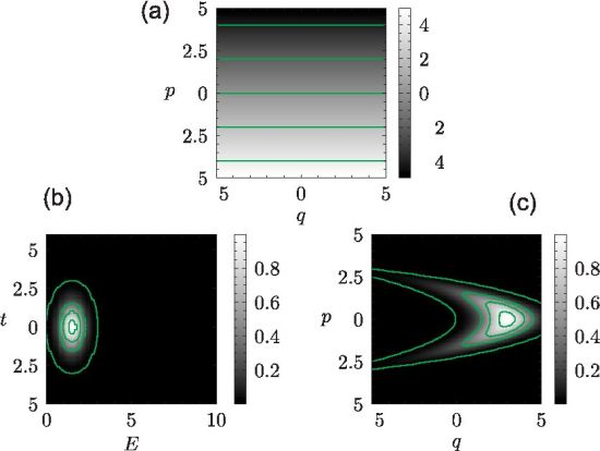
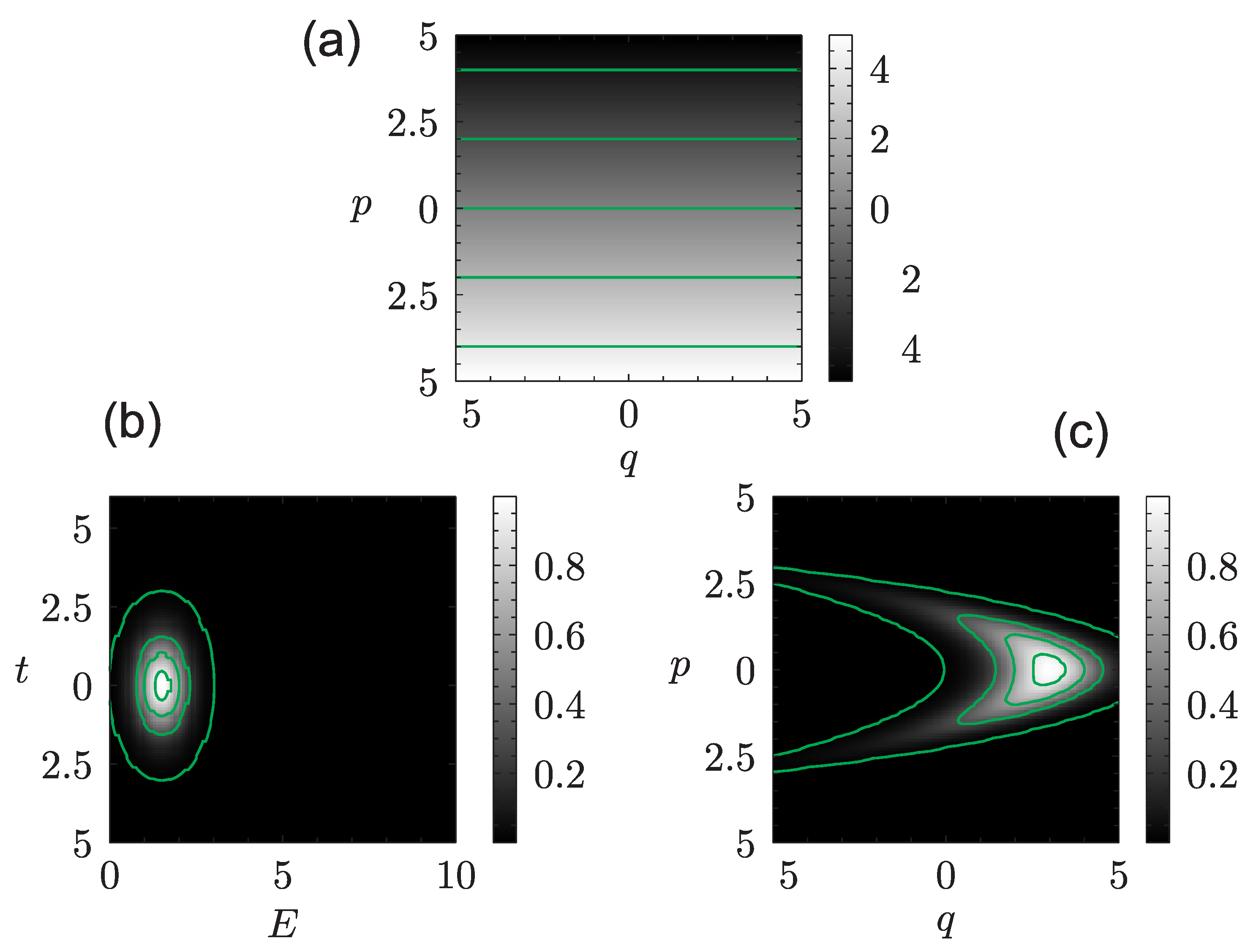
will have another shape and other widths in phase space. In Figure 1, we show plots of the time function, $t\left(z\right)$, for one period, and density plots of the unnormalized energy-time Gaussian probability density in energy-time space and in phase space for the harmonic oscillator. In that calculation, $E_0=1.5$, ${\sigma }_E=0.5$ and ${\sigma }_T=1$.

Figure 1. Time-energy coordinates for the classical Harmonic oscillator. (a) Values of the time function, $t\left(z\right)$, in phase-space; (b) Density plots of an energy-time Gaussian probability density in energy-time space; (c) Density plots of an energy-time Gaussian probability density in phase-space. Here, $E_0=1.5$, ${\sigma }_E=0.5$ and ${\sigma }_t=1$, in dimensionless units.

Figure 1. Time-energy coordinates for the classical Harmonic oscillator. (a) Values of the time function, $t\left(z\right)$, in phase-space; (b) Density plots of an energy-time Gaussian probability density in energy-time space; (c) Density plots of an energy-time Gaussian probability density in phase-space. Here, $E_0=1.5$, ${\sigma }_E=0.5$ and ${\sigma }_t=1$, in dimensionless units.

Let us now consider the linear potential $V\left(q\right)=aq$, where a is a real constant. The time eigencurve for the this potential is given by:

$$\begin{array}{c}\hfill {\gamma }_T\left(t\right)=\left\{z\right|p=-at\}\end{array}$$

(10)

The time variable depends only upon p and a plot of this variable and of the time-energy Gaussian of Equation (9), in time-energy and in phase-space, is shown in Figure 2.

Figure 2. Time-energy coordinates for the classical linear potential. (a) Values of the time function, $t\left(z\right)$; (b) Density plots of an energy-time Gaussian probability density in energy-time space; (c) Density plots of an energy-time Gaussian probability density in phase-space. Here, $E_0=1.5$, ${\sigma }_E=0.5$ and ${\sigma }_T=1$ in dimensionless units.

Figure 2. Time-energy coordinates for the classical linear potential. (a) Values of the time function, $t\left(z\right)$; (b) Density plots of an energy-time Gaussian probability density in energy-time space; (c) Density plots of an energy-time Gaussian probability density in phase-space. Here, $E_0=1.5$, ${\sigma }_E=0.5$ and ${\sigma }_T=1$ in dimensionless units.

We have defined a time coordinate system for classical systems. The method used for that can also be used in quantum systems, as we show below. The advantages of this choice are that the momentum eigenstate at $p=0$ is easy to generate and that it will be formed with all of the energy eigenstates.

In the next section, we will deal with quantum systems, and we will consider both cases, the continuous and the discrete energy spectrum cases. We will also use the linear potential to illustrate the method.

3. Quantum Systems: Continuous Spectrum

Let us consider a one-dimensional quantum system and proceed to obtain time eigenstates, with the linear potential as an illustration of the method.

3.1. Derivation of Time Eigenstates

We will derive time eigenstates for a continuous energy spectrum by the rewriting of the identity operator and by making use of the integral representation of Dirac’s delta function. The main assumption here is that there is a state $|t=0\rangle$, such that $\langle E|t=0\rangle =e^{i\alpha }$, the same value of α for all the energy eigenstates, $|E\rangle$. We will apply the following results to the linear potential.

We start with the expansion of the identity operator in terms of energy eigenstates:

$$\begin{array}{ccc}\hfill \widehat{I}& =& \int dE|E\rangle \langle E|=\int d{E}^{\prime }dE|E^{\prime }\rangle \delta (E-E^{\prime })\langle E|=\int d{E}^{\prime }dE|E^{\prime }\rangle \frac{1}{2\pi \hslash }\int dt{e}^{it(E-E^{\prime })/\hslash }\langle E|\hfill \\ & =& \frac{1}{2\pi \hslash }\int dt\int d{E}^{\prime }dE{e}^{-it\widehat{H}/\hslash }|E^{\prime }\rangle \langle E^{\prime }|t=0\rangle \langle t=0|E\rangle \langle E|e^{it\widehat{H}/\hslash }\hfill \\ & =& \frac{1}{2\pi \hslash }\int dt{e}^{-it\widehat{H}/\hslash }|t=0\rangle \langle t=0|e^{it\widehat{H}/\hslash }\hfill \\ & =& \int dt|t\rangle \langle t|\hfill \end{array}$$

(11)

where we have made use of $1=e^{i\alpha }{e}^{-i\alpha }=\langle E^{\prime }|t=0\rangle \langle t=0|E\rangle$ and where we have defined time eigenstates as:

$$\begin{array}{c}\hfill |t\rangle :=\frac{1}{\sqrt{2\pi \hslash }}{e}^{-it\widehat{H}/\hslash }|t=0\rangle =\frac{1}{\sqrt{2\pi \hslash }}\int dE{e}^{-itE/\hslash }\langle E|t=0\rangle |E\rangle =\frac{e^{i\alpha }}{\sqrt{2\pi \hslash }}\int dE{e}^{-itE/\hslash }|E\rangle \end{array}$$

(12)

Note that we have written the identity operator in terms of time eigenstates $|t\rangle$.

The Hamiltonian is written in terms of time eigenstates as follows:

$$\begin{array}{ccc}\hfill \widehat{H}& =& \int d{E}^{\prime }dE|E^{\prime }\rangle \langle E^{\prime }|\widehat{H}|E\rangle \langle E|\hfill \\ & =& \int d{E}^{\prime }dEE\delta (E^{\prime }-E)|E^{\prime }\rangle \langle E^{\prime }|t=0\rangle \langle t=0|E\rangle \langle E|\hfill \\ & =& \int d{E}^{\prime }dEE\frac{1}{2\pi \hslash }\int dt{e}^{it(E-E^{\prime })/\hslash }|E^{\prime }\rangle \langle E^{\prime }|t=0\rangle \langle t=0|E\rangle \langle E|\hfill \\ & =& \frac{1}{2\pi \hslash }\int dt\int d{E}^{\prime }dEE{e}^{-it\widehat{H}/\hslash }|E^{\prime }\rangle \langle E^{\prime }|t=0\rangle \langle t=0|E\rangle \langle E|e^{it\widehat{H}/\hslash }\hfill \\ & =& \frac{1}{2\pi \hslash }\int dt\int dE{e}^{-it\widehat{H}/\hslash }|t=0\rangle \langle t=0|E\rangle \langle E|\left(-i\hslash \frac{\partial }{\partial t}\right)e^{itE/\hslash }\hfill \\ & =& \int dt|t\rangle \left(-i\hslash \frac{\partial }{\partial t}\right)\langle t|\hfill \end{array}$$

(13)

We now form a time operator as:

$$\begin{array}{ccc}\hfill \widehat{T}& =& \int dt|t\rangle t\langle t|\hfill \\ & =& \int d{E}^{\prime }dE\frac{1}{2\pi \hslash }\int dt{e}^{-it{E}^{\prime }/\hslash }|E^{\prime }\rangle \langle E^{\prime }|t=0\rangle t\langle t=0|E\rangle \langle E|e^{itE/\hslash }\hfill \\ & =& \int d{E}^{\prime }dE\frac{1}{2\pi \hslash }\int dt{e}^{-it{E}^{\prime }/\hslash }\langle E^{\prime }|t=0\rangle \langle t=0|E\rangle |E^{\prime }\rangle \langle E|\left(-i\hslash \frac{\partial }{\partial E}{e}^{itE/\hslash }\right)\hfill \\ & =& -\int d{E}^{\prime }dE\langle E^{\prime }|t=0\rangle \langle t=0|E\rangle |E^{\prime }\rangle \langle E|i\hslash \frac{\partial }{\partial E}\frac{1}{2\pi \hslash }\int dt{e}^{it(E-E^{\prime })/\hslash }\hfill \\ & =& -\int d{E}^{\prime }dE\langle E^{\prime }|t=0\rangle \langle t=0|E\rangle |E^{\prime }\rangle \langle E|i\hslash \frac{\partial }{\partial E}\delta (E-E^{\prime })\hfill \\ & =& -i\hslash \int d{E}^{\prime }\langle E^{\prime }|t=0\rangle \langle t=0|E\rangle |E^{\prime }\rangle \langle E|\delta (E-E^{\prime }){|}_{\mathrm{boundary}}\hfill \\ & & +i\hslash \int d{E}^{\prime }dE\delta (E^{\prime }-E)\frac{\partial }{\partial E}\langle E^{\prime }|t=0\rangle \langle t=0|E\rangle |E^{\prime }\rangle \langle E|\hfill \\ & =& -i\hslash |E\rangle \langle E|{|}_{\mathrm{boundary}}+i\hslash \int d{E}^{\prime }dE\delta (E^{\prime }-E)\frac{\partial }{\partial E}\langle E^{\prime }|t=0\rangle \langle t=0|E\rangle |E^{\prime }\rangle \langle E|\hfill \\ & =& \int dE|E\rangle \left(i\hslash \frac{\partial }{\partial E}\right)\langle E|+\mathrm{b}.\mathrm{t}.\hfill \end{array}$$

(14)

where we have made use of integration by parts and b.t. stands for the boundary terms. For the linear potential, the boundary term vanishes if the wave packet has components in a finite interval of momentum values. With this, we have time and energy representations of the time operator.

When boundary terms can be neglected, the n-th power of $\widehat{T}$ can be written as the integral of $|t\rangle t^n\langle t|$ as:

$$\begin{array}{ccc}\hfill {\widehat{T}}^n& =& \int d{E}^{\prime }\cdots dE|E^{\prime }\rangle \left(i\hslash \frac{\partial }{\partial E^{\prime }}\right)\langle E^{\prime }|\cdots |E\rangle \left(i\hslash \frac{\partial }{\partial E}\right)\langle E|=\int dE|E\rangle {\left(i\hslash \frac{\partial }{\partial E}\right)}^n\langle E|\hfill \\ & =& \int d{E}^{\prime }dE\delta (E^{\prime }-E)|E^{\prime }\rangle {\left(i\hslash \frac{\partial }{\partial E}\right)}^n\langle E|\hfill \\ & =& i\hslash \int d{E}^{\prime }\delta (E^{\prime }-E)|E^{\prime }\rangle {\left(i\hslash \frac{\partial }{\partial E}\right)}^{n-1}\langle E|{|}_{\mathrm{E}\mathrm{boundary}}\hfill \\ & & +\int d{E}^{\prime }dE\left(-i\hslash \frac{\partial \delta (E^{\prime }-E)}{\partial E}\right)|E^{\prime }\rangle {\left(i\hslash \frac{\partial }{\partial E}\right)}^{n-1}\langle E|\hfill \\ & =& \int d{E}^{\prime }dE|E^{\prime }\rangle \langle E|{\left(-i\hslash \frac{\partial }{\partial E}\right)}^n\delta (E^{\prime }-E)+\mathrm{b}.\mathrm{t}.\hfill \\ & =& \int d{E}^{\prime }dE|E^{\prime }\rangle \langle E|{\left(-i\hslash \frac{\partial }{\partial E}\right)}^n\frac{1}{2\pi \hslash }\int dt{e}^{it(E-E^{\prime })/\hslash }\hfill \\ & =& \frac{1}{2\pi \hslash }\int dtd{E}^{\prime }dE|E^{\prime }\rangle \langle E|t^n{e}^{it(E-E^{\prime })/\hslash }\hfill \\ & =& \frac{1}{2\pi \hslash }\int dtd{E}^{\prime }dE{e}^{-it\widehat{H}/\hslash }|E^{\prime }\rangle \langle E^{\prime }|t=0\rangle t^n\langle t=0|E\rangle \langle E|e^{it\widehat{H}/\hslash }\hfill \\ & =& \int dt|t\rangle t^n\langle t|\hfill \end{array}$$

(15)

The time eigenstates Equation (12) are indeed the eigenstates of the time operator Equation (14):

$$\begin{array}{ccc}\hfill \widehat{T}|t\rangle & =& \int dE|E\rangle \left(i\hslash \frac{\partial }{\partial E}\right)\langle E|\frac{1}{\sqrt{2\pi \hslash }}\int d{E}^{\prime }{e}^{-it{E}^{\prime }/\hslash }\langle E^{\prime }|t=0\rangle |E^{\prime }\rangle \hfill \\ & =& \frac{1}{\sqrt{2\pi \hslash }}\int dE|E\rangle \left(i\hslash \frac{\partial }{\partial E}\right)\int d{E}^{\prime }{e}^{-it{E}^{\prime }/\hslash }\langle E^{\prime }|t=0\rangle \langle E|E^{\prime }\rangle \hfill \\ & =& \frac{1}{\sqrt{2\pi \hslash }}\int dE|E\rangle \left(i\hslash \frac{\partial }{\partial E}\right)e^{-itE/\hslash }{e}^{i\alpha }=\frac{1}{\sqrt{2\pi \hslash }}\int dE|E\rangle t{e}^{-itE/\hslash }{e}^{i\alpha }\hfill \\ & =& t|t\rangle \hfill \end{array}$$

(16)

Now, let us see the result of the commutator between the time and Hamiltonian operators. For one of the components of the identity operator, we have that:

$$\begin{array}{ccc}\hfill i\hslash \frac{d}{dt}|t\rangle \langle t|& =& \frac{i\hslash }{2\pi \hslash }\frac{d}{dt}{e}^{-it\widehat{H}/\hslash }|t=0\rangle \langle t=0|e^{it\widehat{H}/\hslash }\hfill \\ & =& \frac{i\hslash }{2\pi \hslash }\left(-\frac{i}{\hslash }\widehat{H}\right)e^{-it\widehat{H}/\hslash }|t=0\rangle \langle t=0|e^{it\widehat{H}/\hslash }+\frac{i\hslash }{2\pi \hslash }{e}^{-it\widehat{H}/\hslash }|t=0\rangle \langle t=0|\left(\frac{i}{\hslash }\widehat{H}\right)e^{it\widehat{H}/\hslash }\hfill \\ & =& \widehat{H}|t\rangle \langle t|-|t\rangle \langle t|\widehat{H}\hfill \\ & =& [\widehat{H},|t\rangle \langle t\left|\right]\hfill \end{array}$$

(17)

Thus:

$$\begin{array}{ccc}\hfill [\widehat{I},\widehat{H}]& =& \int dt\left[\right|t\rangle \langle t|,\widehat{H}]=-\int dti\hslash \frac{d}{dt}|t\rangle \langle t|=-i\hslash |t\rangle \langle t|{|}_{t=-\infty }^{\infty }\hfill \end{array}$$

(18)

and:

$$\begin{array}{ccc}\hfill [\widehat{T},\widehat{H}]& =& \int dt\left[\right|t\rangle t\langle t|,\widehat{H}]=-\int dtti\hslash \frac{d}{dt}|t\rangle \langle t|=-i\hslash t|t\rangle \langle t|{|}_{t=-\infty }^{\infty }+i\hslash \int dt|t\rangle \langle t|\frac{dt}{dt}\hfill \\ & =& i\hslash \widehat{I}-i\hslash t|t\rangle \langle t|{|}_{t=-\infty }^{\infty }\hfill \end{array}$$

(19)

Since the Hilbert space is composed of ${\mathcal{L}}^2$ functions, we expect that in energy-time space, the wave function will also be of an integrable square type and, then, the boundary terms will vanish. This leads to the conclusion that $\widehat{I}$ and $\widehat{T}$ have the desired commutator with $\widehat{H}$.

3.2. Equalities Involving Powers of Time

We can write down an expression for any power of t:

$$\begin{array}{c}\hfill \left[\int dt{t}^{n+1}|t\rangle \langle t|,\widehat{H}\right]=-i\hslash \int dt{t}^{n+1}\frac{d}{dt}|t\rangle \langle t|=-i\hslash t^{n+1}|t\rangle \langle t|{|}_{-\infty }^{\infty }+i\hslash \int dt\frac{d{t}^{n+1}}{dt}|t\rangle \langle t|\end{array}$$

(20)

i.e., we have that:

$$\begin{array}{c}\hfill \left[{\widehat{T}}^{n+1},\widehat{H}\right]=i\hslash (n+1){\widehat{T}}^n\end{array}$$

(21)

where ${\widehat{T}}^n:=\int dt{t}^n|t\rangle \langle t|$. This equality is consistent with the constant commutator being a derivation.

From the above equality, it is easy to show, by the induction method, that:

$$\begin{array}{c}\hfill \underset{n}{\underbrace{\left[\cdots \left[{\widehat{T}}^n,\widehat{H}\right],\cdots ,\widehat{H}\right]}}=n!{\left(i\hslash \right)}^n\end{array}$$

(22)

3.3. Change of Representation

We can obtain the energy eigenvector from the time eigenvectors as follows:

$$\begin{array}{ccc}\hfill \int dt{e}^{iEt/\hslash }{\langle E|t=0\rangle }^{*}|t\rangle & =& \frac{1}{2\pi \hslash }\int dt{e}^{iEt/\hslash }{\langle E|t=0\rangle }^{*}{e}^{-it\widehat{H}/\hslash }\int d{E}^{\prime }\langle E^{\prime }|t=0\rangle |E^{\prime }\rangle \hfill \\ & =& \int d{E}^{\prime }\frac{{\langle E|t=0\rangle }^{*}}{2\pi \hslash }\int dt{e}^{i(E-E^{\prime })t/\hslash }\langle E^{\prime }|t=0\rangle |E^{\prime }\rangle \hfill \\ & =& \int d{E}^{\prime }{\langle E|t=0\rangle }^{*}\delta (E-E^{\prime })\langle E^{\prime }|t=0\rangle |E^{\prime }\rangle \hfill \\ & =& |E\rangle \hfill \end{array}$$

(23)

and vice-versa, from the definition, we can see that the appropriate sum of energy eigenstates results in the time eigenstate:

$$\begin{array}{c}\hfill \int dE\frac{e^{-itE/\hslash }}{\sqrt{2\pi \hslash }}\langle E|t=0\rangle |E\rangle =\frac{e^{-it\widehat{H}/\hslash }}{\sqrt{2\pi \hslash }}\int dE\langle E|t=0\rangle |E\rangle =|t\rangle \end{array}$$

(24)

3.4. Orthogonality between Time Eigenstates

The time eigenstates are not orthogonal for the same zero time state:

$$\begin{array}{ccc}\hfill \langle t^{\prime }|t\rangle & =& \frac{1}{2\pi \hslash }\langle t=0|e^{i{t}^{\prime }\widehat{H}/\hslash }{e}^{-it\widehat{H}/\hslash }|t=0\rangle =\frac{1}{2\pi \hslash }\langle t=0|e^{-i(t-t^{\prime })\widehat{H}/\hslash }|t=0\rangle =\langle t=0|t-t^{\prime }\rangle \hfill \end{array}$$

(25)

However, assuming that there is a set of zero-time eigenstates that are orthogonal, these states are indeed orthogonal when t is the same and the zero time states are different:

$$\begin{array}{ccc}\hfill \langle t=0;{\tau }^{\prime }|t=0;\tau \rangle & =& \int d{E}^{\prime }dE\langle E^{\prime }|\langle t=0;{\tau }^{\prime }|E^{\prime }\rangle \frac{e^{it\widehat{H}/\hslash }{e}^{-it\widehat{H}/\hslash }}{2\pi \hslash }\langle E|t=0;\tau \rangle |E\rangle \hfill \\ & =& \frac{1}{2\pi \hslash }\int d{E}^{\prime }dE\langle t=0;{\tau }^{\prime }|E^{\prime }\rangle \langle E^{\prime }|E\rangle \langle E|t=0;\tau \rangle \hfill \\ & =& \frac{1}{2\pi \hslash }\int dE\langle t=0;{\tau }^{\prime }|E\rangle \langle E|t=0;\tau \rangle \hfill \\ & =& \frac{1}{2\pi \hslash }\delta ({\tau }^{\prime }-\tau )\hfill \end{array}$$

(26)

where τ is a parameter that distinguishes between the different zero time eigenstates.

4. Quantum Systems: Discrete Spectrum

We need to consider a discrete version of the above results, so that we can handle the cases of discrete spectrum and discretized versions of a continuous spectrum model system. In this section, we introduce time eigenstates for systems with a discrete spectrum.

4.1. Derivation of Time Eigenstates

Again, to obtain time eigenstates, we rewrite the identity operator, written as an energy eigenstates expansion, using an approximation to Kronecker’s delta with $sin\left(x\right)/x$, and later, we use the integral representation of this function.

For some large $T\in \mathbb{R}$, and denoting by $|n\rangle$ the eigenvectors of the Hamiltonian operator, we have that:

$$\begin{array}{ccc}\hfill \widehat{I}\left(T\right)& =& \sum _n|n\rangle \langle n|=\sum _{m,n}|m\rangle {\delta }_{mn}\langle n|\approx \sum _{m,n}|m\rangle \frac{2\hslash }{T(E_n-E_m)}sin\left(\frac{T(E_n-E_m)}{2\hslash }\right)\langle n|\hfill \\ & =& \sum _{m,n}|m\rangle \frac{1}{T}{\int }_{-T/2}^{T/2}dt{e}^{it(E_n-E_m)/\hslash }\langle n|=\frac{1}{T}{\int }_{-T/2}^{T/2}dt\sum _{m,n}{e}^{-it\widehat{H}/\hslash }|m\rangle \langle n|e^{it\widehat{H}/\hslash }\hfill \\ & =& \frac{1}{T}{\int }_{-T/2}^{T/2}dt|t\rangle \langle t|\hfill \end{array}$$

(27)

This defines time eigenstates of the form:

$$|t\rangle =e^{-it\widehat{H}/\hslash }|t=0\rangle ,|t=0\rangle =\sum _m|m\rangle$$

(28)

Note that if there is a state $|t=0\rangle$, such that $\langle n|t=0\rangle =e^{i\alpha }$, we can take it as a zero time eigenstate, and then, we can additionally do the following:

$$\begin{array}{ccc}\hfill \widehat{I}\left(T\right)& =& \frac{1}{T}{\int }_{-T/2}^{T/2}dt\sum _{m,n}{e}^{-it\widehat{H}/\hslash }|m\rangle \langle m|t=0\rangle \langle t=0|n\rangle \langle n|e^{it\widehat{H}/\hslash }\hfill \\ & =& \frac{1}{T}{\int }_{-T/2}^{T/2}dt|t\rangle \langle t|\hfill \end{array}$$

(29)

where we now have defined time eigenstates as:

$$\begin{array}{c}\hfill |t\rangle :=e^{-it\widehat{H}/\hslash }|t=0\rangle =\sum _m{e}^{-it{E}_m/\hslash }\langle m|t=0\rangle |m\rangle \end{array}$$

(30)

The advantage of this definition is that the time eigenstate can be more specific than just the sum of all of the energy eigenstates. The following properties hold for the second type of time eigenstate.

We form a T-dependent time operator as:

$$\begin{array}{ccc}\hfill \widehat{T}\left(T\right)& =& \frac{1}{T}{\int }_{-T/2}^{T/2}dt|t\rangle t\langle t|=\sum _{m,n}\frac{1}{T}{\int }_{-T/2}^{T/2}dt{e}^{-it{E}_m/\hslash }|m\rangle \langle m|t=0\rangle t\langle t=0|n\rangle \langle n|e^{it{E}_n/\hslash }\hfill \\ & =& \sum _{m,n}\frac{1}{T}{\int }_{-T/2}^{T/2}dtt{e}^{it(E_n-E_m)/\hslash }\langle m|t=0\rangle \langle t=0|n\rangle |m\rangle \langle n|\hfill \\ & =& \sum _{m\ne n}\frac{i\hslash }{E_n-E_m}\left[\frac{2\hslash }{T(E_n-E_m)}sin\left(\frac{T(E_n-E_m)}{2\hslash }\right)-cos\left(\frac{T(E_n-E_m)}{2\hslash }\right)\right]|m\rangle \langle n|\hfill \end{array}$$

(31)

The domain of this operator is the Hilbert space. With this equality, we have time and energy representations of the time operator. This time operator is similar to the operator used by Galapon [74] and later analyzed by Arai et al. [75,76]. However, Galapon’s operator does not make use of the oscillating factors; they do not give expressions for the time eigenvectors, and their operator is valid only in a limited domain.

The above defined operators have the expected commutators with $\widehat{H}$, for wave functions with a finite support in time. The time derivative of one component is:

$$\begin{array}{c}\hfill i\hslash \frac{d}{dt}|t\rangle \langle t|=-i\hslash \frac{i}{\hslash }\widehat{H}|t\rangle \langle t|+i\hslash |t\rangle \langle t|\frac{i}{\hslash }\widehat{H}=[\widehat{H},|t\rangle \langle t\left|\right]\end{array}$$

(32)

This equality allows us to find what the commutator between $\widehat{I}\left(T\right)$ and $\widehat{H}$ is:

$$\begin{array}{c}\hfill [\widehat{I}\left(T\right),\widehat{H}]=\frac{1}{T}{\int }_{-T/2}^{T/2}dt\left[\right|t\rangle \langle t|,\widehat{H}]=-\frac{1}{T}{\int }_{-T/2}^{T/2}dti\hslash \frac{d}{dt}|t\rangle \langle t|=-i\hslash \frac{1}{T}|t\rangle \langle t|{|}_{t=-\infty }^{\infty }\end{array}$$

(33)

and:

$$\begin{array}{ccc}\hfill [\widehat{T}\left(T\right),\widehat{H}]& =& \frac{1}{T}{\int }_{-T/2}^{T/2}dt\left[\right|t\rangle t\langle t|,\widehat{H}]=-\frac{1}{T}{\int }_{-T/2}^{T/2}dtti\hslash \frac{d}{dt}|t\rangle \langle t|\hfill \\ & =& -i\hslash \frac{t}{T}|t\rangle \langle t|{|}_{t=-\infty }^{\infty }+\frac{1}{T}{\int }_{-T/2}^{T/2}dt|t\rangle \langle t|i\hslash \frac{dt}{dt}=-i\hslash \frac{1}{T}|t\rangle \langle t|{|}_{t=-\infty }^{\infty }+i\hslash \widehat{I}\left(T\right)\hfill \end{array}$$

(34)

It is easy to see that the time operator, $\widehat{T}\left(T\right)$, is self adjoint and that the eigenoperator of the commutator, $[\widehat{T},•]$, is the propagator, i.e.,

$$\begin{array}{c}\hfill [\widehat{T},e^{-i\tau \widehat{H}/\hslash }]=\tau e^{-i\tau \widehat{H}/\hslash }\end{array}$$

(35)

Based on the last equality, we can show that the time eigenstate Equation (30) is indeed an eigenstate of the time operator Equation (31).

$$\begin{array}{ccc}\hfill t|t\rangle & =& t{e}^{-it\widehat{H}/\hslash }|t=0\rangle =[\widehat{T},e^{-it\widehat{H}/\hslash }]|t=0\rangle =\widehat{T}{e}^{-it\widehat{H}/\hslash }|t=0\rangle -e^{-it\widehat{H}/\hslash }\widehat{T}|t=0\rangle =\widehat{T}|t\rangle \hfill \end{array}$$

(36)

where we have made use of the fact that $|t=0\rangle$ is the time eigenstate with eigenvalue zero.

For the Hamiltonian, we have that:

$$\begin{array}{ccc}\hfill \widehat{H}& =& \sum _{m,n}|m\rangle \langle m|\widehat{H}|n\rangle \langle n|=\sum _{mn}{E}_n{\delta }_{mn}|m\rangle \langle m|t=0\rangle \langle t=0|n\rangle \langle n|\hfill \\ & \approx & \sum _{mn}{E}_n\frac{2\hslash }{T(E_n-E_m)}sin\left(\frac{T(E_n-E_m)}{2\hslash }\right)|m\rangle \langle m|t=0\rangle \langle t=0|n\rangle \langle n|\hfill \\ & =& \sum _{mn}\frac{E_n}{T}{\int }_{-T/2}^{T/2}dt{e}^{it(E_n-E_m)/\hslash }|m\rangle \langle m|t=0\rangle \langle t=0|n\rangle \langle n|\hfill \\ & =& \sum _{mn}\frac{1}{T}{\int }_{-T/2}^{T/2}dt{e}^{-it{E}_m/\hslash }|m\rangle \langle m|t=0\rangle \left(-i\hslash \frac{\partial }{\partial t}\right)\langle t=0|n\rangle \langle n|e^{it{E}_n/\hslash }\hfill \\ & =& \frac{1}{T}{\int }_{-T/2}^{T/2}dt|t\rangle \left(-i\hslash \frac{\partial }{\partial t}\right)\langle t|\hfill \end{array}$$

(37)

as expected.

The discrete version of the time operator has the same properties as the continuous counterpart. Some of them follow.

4.2. Change of Representation

We can obtain the energy eigenvector from the time eigenvectors as follows:

$$\begin{array}{ccc}\hfill \frac{1}{T}{\int }_{-T/2}^{T/2}dt{e}^{i{E}_{n}t/\hslash }{\langle n|t=0\rangle }^{*}|t\rangle & =& \frac{1}{T}{\int }_{-T/2}^{T/2}dt{e}^{i{E}_{n}t/\hslash }{\langle n|t=0\rangle }^{*}{e}^{-it\widehat{H}/\hslash }\sum _m\langle m|t=0\rangle |m\rangle \hfill \\ & =& \sum _m\frac{1}{T}{\int }_{-T/2}^{T/2}dt{e}^{i(E_n-E_m)t/\hslash }{\langle n|t=0\rangle }^{*}\langle m|t=0\rangle |m\rangle \hfill \\ & =& \sum _m\frac{2\hslash }{T(E_n-E_m)}sin\left(\frac{T(E_n-E_m)}{2\hslash }\right)|m\rangle \hfill \\ & \underset{T\to \infty }{⟶}& |n\rangle \hfill \end{array}$$

(38)

and vice-versa, from the definition, we can see that the appropriate sum of energy eigenstates results in the time eigenstate:

$$\begin{array}{ccc}\hfill \sum _n{e}^{-it{E}_n/\hslash }\langle n|t=0\rangle |n\rangle & =& e^{-it\widehat{H}/\hslash }\sum _n\langle n|t=0\rangle |n\rangle =|t\rangle \hfill \end{array}$$

(39)

4.3. Orthogonality between Time Eigenstates

The time eigenstates are not orthogonal for the same zero time eigenstate:

$$\begin{array}{ccc}\hfill \langle t^{\prime }|t\rangle & =& \langle t=0|e^{i{t}^{\prime }\widehat{H}/\hslash }{e}^{-it\widehat{H}/\hslash }|t=0\rangle \hfill \\ & =& \langle t=0|e^{-i(t-t^{\prime })\widehat{H}/\hslash }|t=0\rangle =\langle t=0|t-t^{\prime }\rangle \hfill \end{array}$$

(40)

However, the time eigenstates are indeed orthogonal between two eigenstates when t is the same and the zero time states are different:

$$\begin{array}{ccc}\hfill \langle t=0;{\tau }^{\prime }|t=0;\tau \rangle & =& \sum _{mn}\langle m|\langle t=0;{\tau }^{\prime }|m\rangle e^{it\widehat{H}/\hslash }{e}^{-it\widehat{H}/\hslash }\langle n|t=0;\tau \rangle |n\rangle \hfill \\ & =& \sum _{mn}\langle t=0;{\tau }^{\prime }|m\rangle \langle m|n\rangle \langle n|t=0;\tau \rangle =\sum _n\langle t=0;{\tau }^{\prime }|n\rangle \langle n|t=0;\tau \rangle \hfill \\ & =& \delta ({\tau }^{\prime }-\tau )\hfill \end{array}$$

(41)

where τ is a parameter that differentiates the $|t=0\rangle$ states and where we have assumed that they are orthonormal.

5. Matrix Elements of Operators

A calculation that can be used to verify our results is the matrix elements of operators. It is also interesting, by itself, to find the matrix elements of the time operator. Therefore, in this section, we calculate these matrix elements in coordinate space. These matrix elements are easy to calculate once we have the energy eigenstates at our disposal, since identity, Hamiltonian and time operators have been written in terms of them. What we need is the energy eigenstates in coordinate and momentum representations.

We calculate the matrix elements of quantum operators for the linear potential with $a=1$ and Hamiltonian:

$$\widehat{H}=\frac{1}{2m}{\widehat{P}}^2+a\widehat{Q}$$

(42)

For numerical calculations, we will use a discretized version of the spectrum, and we will work in the energy interval, $E\in (-40,40)$. The unnormalized energy eigenfunction for the linear potential, in the momentum representation, is:

$${\varphi }_E\left(p\right)=e^{-iEp/a\hslash +i{p}^3/6am\hslash }$$

(43)

This function complies with the requirement of $\langle E|p\rangle =e^{i\alpha }$ when $p=0$, as is needed for the results of this paper. Thus, this is our zero-time eigenstate.

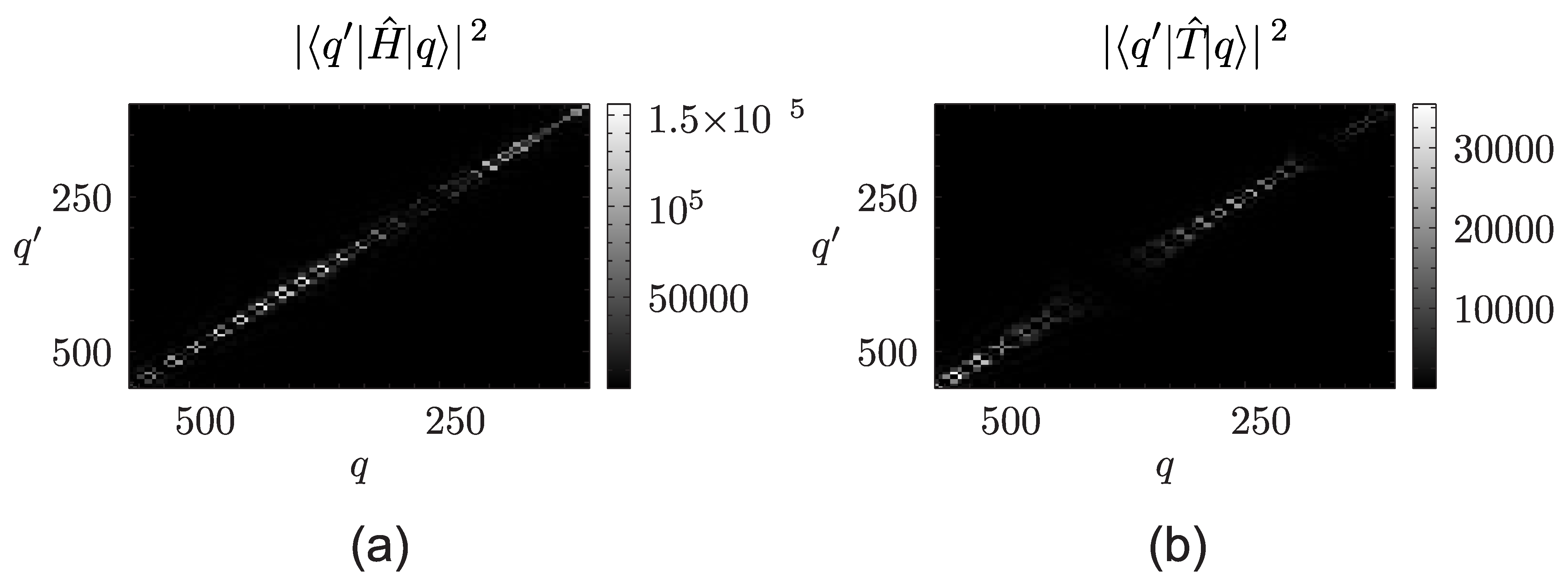
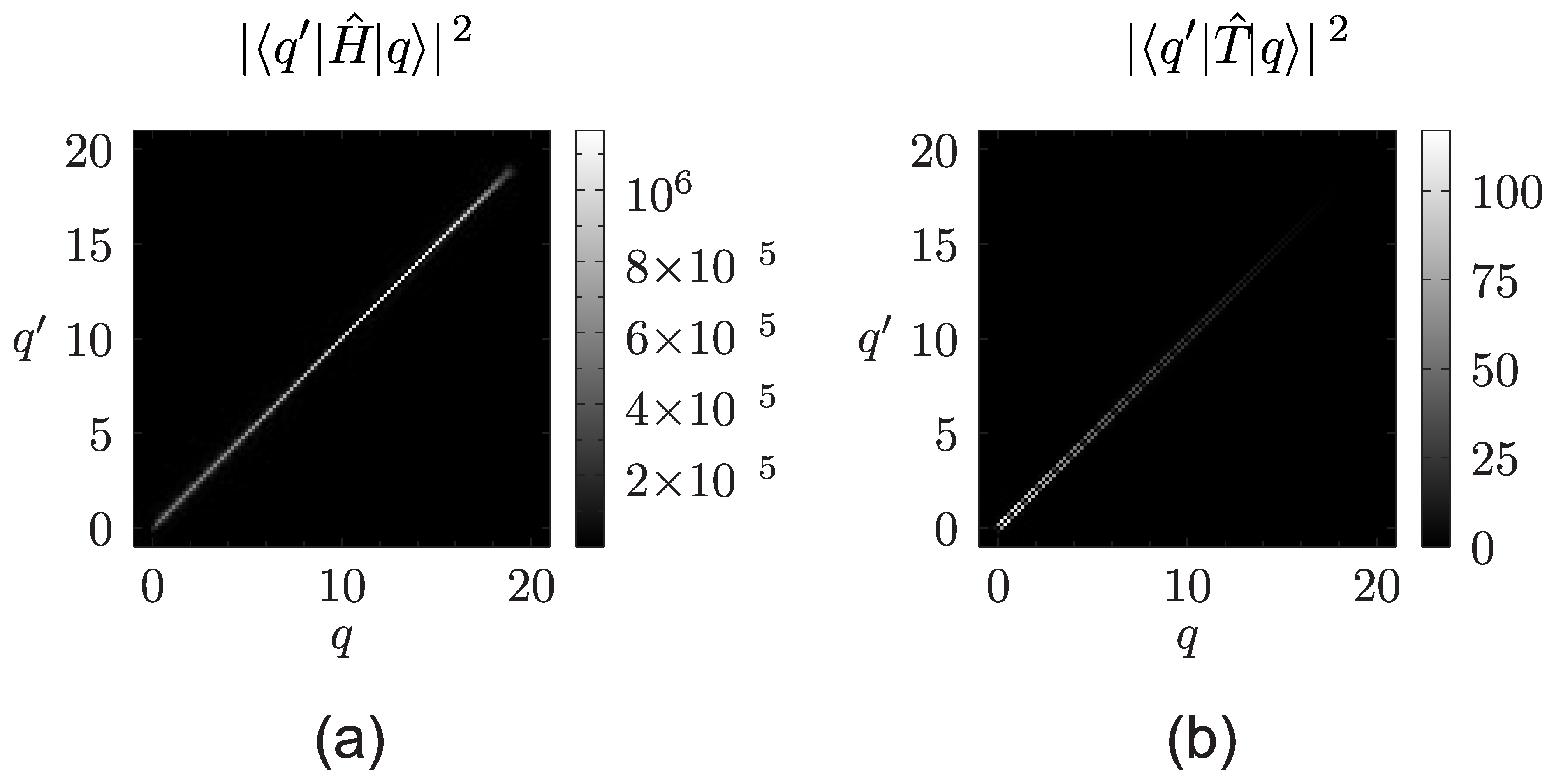
By using the results of Section 4, we have made density plots of the squared magnitude of the coordinate matrix elements of operators, which are shown in Figure 3. The matrix representation of these operators is diagonal or near diagonal for the time operator. The Hamiltonian and time matrix elements oscillate, and the time operator has higher values for large negative values of q.

Figure 3. (a) Density plots of the squared magnitude of the coordinate matrix elements of the Hamiltonian ; (b) time operators for the linear potential $V\left(q\right)=aq$ with $a=1$.

Figure 3. (a) Density plots of the squared magnitude of the coordinate matrix elements of the Hamiltonian ; (b) time operators for the linear potential $V\left(q\right)=aq$ with $a=1$.

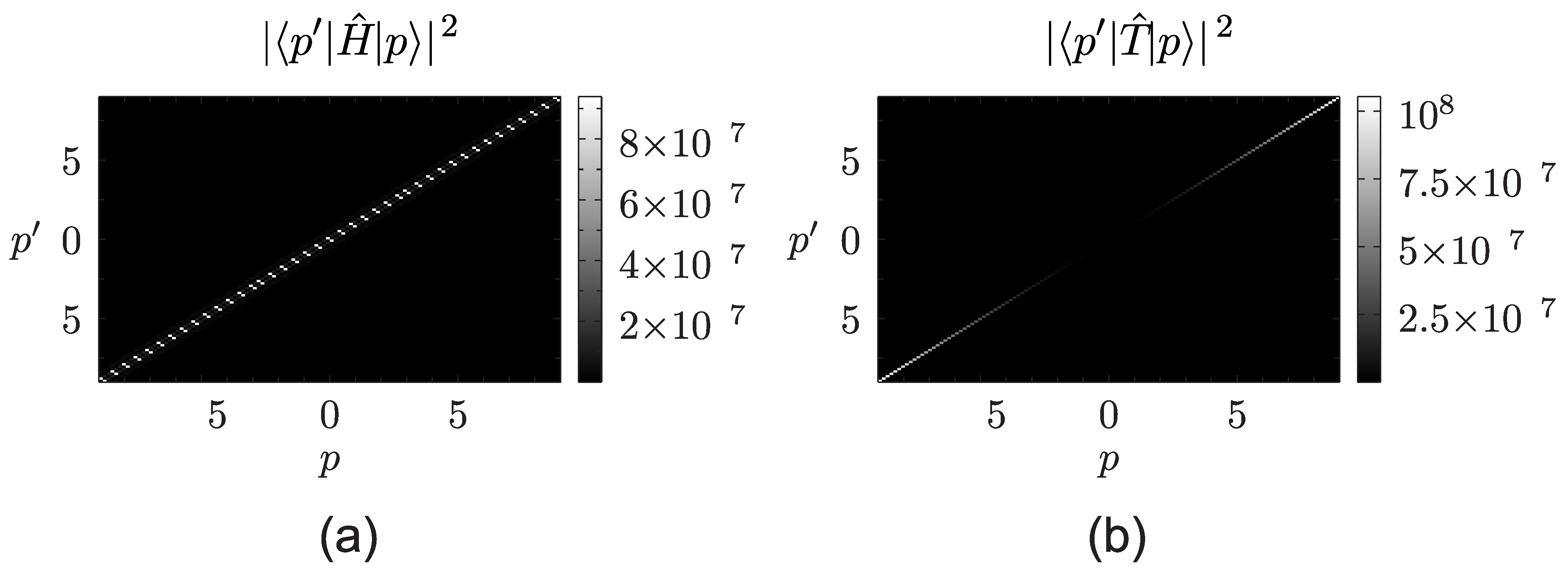
The squared magnitude of the matrix elements of operators in the momentum representation is shown in Figure 4. We notice that the values of the squared magnitude of the matrix elements of the time operator increases with the increase of the magnitude of the momentum.

Figure 4. (a) Density plots of the squared magnitude of the momentum matrix elements of the Hamiltonian; (b) time operators for the linear potential $V\left(q\right)=aq$ with $a=1$.

Figure 4. (a) Density plots of the squared magnitude of the momentum matrix elements of the Hamiltonian; (b) time operators for the linear potential $V\left(q\right)=aq$ with $a=1$.

In Figure 5, there are density plots of the squared magnitude of coordinate matrix elements of operators for the harmonic oscillator. When the value $T=\pi$ is used, we obtain the matrix representation of the operators for positive coordinate, but if we use the value $T=2\pi$, we obtain the matrix elements for all values of q. As always, the matrix elements for the identity and for the Hamiltonian are diagonal in the coordinate representation and around the diagonal for the time operator.

Figure 5. Density plots of the squared magnitude of the coordinate matrix elements of some operators for the harmonic oscillator. On left, the Hamiltonian operator, and on right, the time operator. We have used $T=\pi$. The matrix elements extend to negative coordinates when $T=2\pi$. We have used 50 energy eigenfunctions for these plots.

Figure 5. Density plots of the squared magnitude of the coordinate matrix elements of some operators for the harmonic oscillator. On left, the Hamiltonian operator, and on right, the time operator. We have used $T=\pi$. The matrix elements extend to negative coordinates when $T=2\pi$. We have used 50 energy eigenfunctions for these plots.

6. Remarks

We have shown how to define a time coordinate system in phase space for classical systems. Any hypersurface that crosses the energy shells can be used as a zero time surface, but the surfaces introduced in [73] and in this paper are easy to use for any potential function with the additional advantage that the same process can be used for quantum systems.

Our operator and states comply with the desired properties for a time operator and its eigenstates. The time eigenstates are similar to coordinate and momentum eigenstates in that they are not normalizable at all, and therefore, are not part of the Hilbert space, but the domain of the time operator is indeed the Hilbert space. In a similar way as the coordinate and momentum eigenstates, the time eigenstates can be used as an alternative coordinate for classical and quantum systems. Thus, we can adopt the point of view that energy and time are an alternative coordinate system similar to coordinate and momentum variables.

The coordinate matrix elements of the identity, Hamiltonian and time operators, in the time eigenstates basis, support our results. They also have the expected properties.

For systems with higher dimension than one, the zero-time eigencurve is a hypersurface with one of the components of the momentum equal to zero. The evolution of that curve generates the time coordinate system in phase space.

With these results, we are starting to solve a series of old puzzles in Quantum Mechanics, puzzles that are also present in Classical Mechanics.

References

- Holevo, A.S. Probabilistic and Statistical Aspects of Quantum Theory; North-Holland: Amsterdam, The Netherlands, 1982. [Google Scholar]
- Grot, N.; Rovelli, C.; Tate, R.S. Time of arrival in quantum mechanics. Phys. Rev. A 1996, 54, 4676–4690. [Google Scholar] [CrossRef] [PubMed]
- Rovelli, C. Quantum mechanics without time: A model. Phys. Rev. D 1990, 42, 2638–2646. [Google Scholar] [CrossRef]
- Rovelli, C. Time in quantum gravity: An hypothesis. Phys. Rev. D 1991, 43, 442–456. [Google Scholar] [CrossRef]
- Kijowski, J. On the time operator in quantum mechanics and the Heisenberg uncertainty relation for energy and time. Rep. Math. Phys. 1974, 6, 361–386. [Google Scholar] [CrossRef]
- Hegerfeldt, G.C.; Muga, J.G.; Muñoz, J. Manufacturing time operators: Covariance, selection criteria, and examples. Phys. Rev. A 2010, 82, 012113. [Google Scholar] [CrossRef]
- Jaffé, C.; Brumer, P. Classical liouville mechanics and intramolecular relaxation dynamics. J. Phys. Chem. 1984, 88, 4829–4839. [Google Scholar] [CrossRef]
- Muga, J.G.; Sala-Mayato, R.; Egusquiza, I.L. (Eds.) Time in Quantum Mechanics; Springer: Berlin, Germany, 2008; Lecture Notes in Physics; Volume 734.
- Muga, J.G.; Leavens, C.R. Arrival time in quantum mechanics. Phys. Rep. 2000, 338, 353–438. [Google Scholar] [CrossRef]
- Galapon, E.A. Paulis theorem and quantum canonical pairs: The consistency of a bounded, self-adjoint time operator canonically conjugate to a Hamiltonian with non-empty point spectrum. Proc. R. Soc. Lond. A 2002, 458, 451–472. [Google Scholar] [CrossRef]
- Sombillo, D.L.B.; Galapon, E.A. Quantum time of arrival Goursat problem. J. Math. Phys. 2012, 53, 043702. [Google Scholar] [CrossRef]
- Pauli, W. Handbuch der Physik, 1st ed.; Geiger, H., Scheel, K., Eds.; Springer: Berlin, Germany, 1926; Volume 23. [Google Scholar]
- De la Madrid, R.; Isidro, J.M. The HFT selfadjoint variant of time operators. Adv. Stud. Theor. Phys. 2008, 2, 281–289. [Google Scholar]
- Razavy, M. Time of arrival operator. Can. J. Phys. 1971, 49, 3075–3081. [Google Scholar] [CrossRef]
- Razavy, M. Quantum-mechanical time operator. Am. J. Phys. 1967, 35, 955–960. [Google Scholar] [CrossRef]
- Isidro, J.M. Bypassing Paulis theorem. Phys. Lett. A 2005, 334, 370–375. [Google Scholar] [CrossRef]
- Muga, J.G. The time of arrival concept in quantum mechanics. Superlattices Microstruct. 1998, 23, 833–842. [Google Scholar] [CrossRef]
- Torres-Vega, G. Marginal picture of quantum dynamics related to intrinsic arrival times. Phys. Rev. A. 2007, 76, 032105. [Google Scholar] [CrossRef]
- Torres-Vega, G. Energy-time representation for quantum systems. Phys. Rev. A. 2007, 75, 032112. [Google Scholar] [CrossRef]
- Torres-Vega, G. Quantum-like picture for intrinsic, classical, arrival distributions. J. Phys. A 2009, 42, 465307. [Google Scholar] [CrossRef]
- Torres-Vega, G. Dynamics as the preservation of a constant commutator. Phys. Lett. A 2007, 369, 384–392. [Google Scholar] [CrossRef]
- Torres-Vega, G. Correspondence, Time, Energy, Uncertainty, Tunnelling, and Collapse of Probability Densities. In Theoretical Concepts of Quantum Mechanics; Pahlavani, M.R., Ed.; InTech: Rijeka, Croatia, 2012; Chapter 4. [Google Scholar]
- Torres-Vega, G. Classical and Quantum Conjugate Dynamics—The Interplay Between Conjugate Variables. In Advances in Quantum Mechanics; Bracken, P., Ed.; InTech: Rijeka, Croatia, 2013; Chapter 1. [Google Scholar]
- Jaffé, C.; Brumer, P. Classical-quantum correspondence in the distribution dynamics of integrable systems. J. Chem. Phys. 1985, 82, 2330–2340. [Google Scholar] [CrossRef]
- Bokes, P. Time operators in stroboscopic wave-packet basis and the time scales in tunneling. Phys. Rev. A 2011, 83, 032104. [Google Scholar] [CrossRef]
- Bokes, P.; Corsetti, F.; Godby, R.W. Stroboscopic wave-packet description of nonequilibrium many-electron problems. Phys. Rev. Lett. 2008, 101, 046402. [Google Scholar] [CrossRef] [PubMed]
- Bokes, P.; Corsetti, F.; Godby, R.W. Stroboscopic wavepacket description of non-equilibrium many-electron problems: Demonstration of the convergence of the wavepacket basis. 2008; arXiv:0803.2448. [Google Scholar]
- Baute, A.D.; Sala Mayato, R.; Palao, J.P.; Muga, J.G.; Egusquiza, I.L. Time of arrival distribution for arbitrary potentials and Wigner’s time-energy uncertainty relation. Phys. Rev. A 2000, 61, 022118. [Google Scholar] [CrossRef]
- Giannitrapani, R. Positive-operator-valued time observable in quantum mechanics. Int. J. Theor. Phys. 1997, 36, 1575–1584. [Google Scholar] [CrossRef]
- Kobe, D.H. Canonical transformation to energy and “tempus” in classical mechanics. Am. J. Phys. 1993, 61, 1031–1037. [Google Scholar] [CrossRef]
- Kobe, D.H.; Aguilera-Navarro, V.C. Derivation of the energy-time uncertainty relation. Phys. Rev. A 1994, 50, 933–938. [Google Scholar] [CrossRef] [PubMed]
- Rosenbaum, D.M. Super Hilbert space and the quantum-mechanical time operators. J. Math. Phys. 1969, 10, 1127–1144. [Google Scholar] [CrossRef]
- Johns, O.D. Canonical transformation with time as a coordinate. Am. J. Phys. 1989, 57, 204–215. [Google Scholar] [CrossRef]
- Leavens, C.R. Time of arrival in quantum and Bohmian mechnaics. Phys. Rev. A 1998, 58, 840–847. [Google Scholar] [CrossRef]
- Lippmann, B.A. Operator for time delay induced by scattering. Phys. Rev. 1966, 151, 1023–1024. [Google Scholar] [CrossRef]
- Werner, R.F. Wigner quantisation of arrival time and oscillator phase. J. Phys. A 1988, 21, 4565–4575. [Google Scholar] [CrossRef]
- Marshall, T.W.; Watson, E.J. A drop of ink falls from my pen...It comes to earth, I know not when. J. Phys. A 1985, 18, 3531–3559. [Google Scholar] [CrossRef]
- Wigner, E.P. Lower limit for the energy derivative of the scattering phase shift. Phys. Rev. 1955, 98, 145–147. [Google Scholar] [CrossRef]
- Allcock, G.R. The time of arrival in quantum mechanics I. Formal considerations. Ann. Phys. 1969, 53, 253–285. [Google Scholar] [CrossRef]
- Allcock, G.R. The time of arrival in quantum mechanics II. The individual measurement. Ann. Phys. 1969, 53, 286–310. [Google Scholar] [CrossRef]
- Allcock, G.R. The time of arrival in quantum mechanics III. The measurement ensemble. Ann. Phys. 1969, 53, 311–348. [Google Scholar] [CrossRef]
- Delgado, V. Probability distribution of arrival times in quantum mechanics. Phys. Rev. A 1998, 57, 762–770. [Google Scholar] [CrossRef]
- Delgado, V.; Muga, J.G. Arrival time in quantum mechanics. Phys. Rev. A 1997, 56, 3425–3435. [Google Scholar] [CrossRef]
- Halliwell, J.J. Arrival time in quantum theory from an irreversible detector model. Prog. Theor. Phys. 1999, 102, 707–717. [Google Scholar] [CrossRef]
- Muga, J.G.; Baute, A.D.; Damborenea, J.A.; Egusquiza, I.L. Model for the arrival-time distribution in fluorescence time-of-flight experiments. 2000; arXiv:quant-ph/0009111. [Google Scholar]
- Galapon, E.A.; Caballar, R.F.; Bahague, R.T., Jr. Confined quantum time of arrivals. Phys. Rev. Lett. 2004, 93, 180406. [Google Scholar] [CrossRef] [PubMed]
- Eric, A.; Galapon, F.; Delgado, J.; Gonzalo, M.; Iñigo, E. Transition from discrete to continuous time-of-arrival distribution for a quantum particle. Phys. Rev. A 2005, 72, 042107. [Google Scholar]
- Galapon, E.A.; Caballar, R.F.; Bahague, R.T., Jr. Confined quantum time of arrival for the vanishing potential. Phys. Rev. A 2005, 72, 062107. [Google Scholar] [CrossRef]
- Galapon, E.A. What could have we been missing while Pauli’s theorem was in force? 2003; arXiv:quant-ph/0303106. [Google Scholar]
- Muga, J.G.; Leavens, C.R.; Palao, J.P. Space-time properties of free-motion time-of-arrival eigenfunctions. Phys. Rev. A 1998, 58, 4336–4344. [Google Scholar] [CrossRef]
- Skulimowski, M. Construction of time covariant POV measures. Phys. Lett. A 2002, 297, 129–136. [Google Scholar] [CrossRef]
- Damborenea, J.A.; Egusquiza, I.L.; Hegerfeldt, G.C.; Muga, J.G. Measurement-based approach to quantum arrival times. Phys. Rev. A 2002, 66, 052104. [Google Scholar] [CrossRef]
- Baute, A.D.; Egusquiza, I.L.; Muga, J.G. Time of arrival distributions for interaction potentials. Phys. Rev. A 2001, 64, 012501. [Google Scholar] [CrossRef]
- Brunetti, R.; Fredenhagen, K. Time of occurrence observable in quantum mechanics. Phys. Rev. A 2002, 66, 044101. [Google Scholar] [CrossRef]
- Hegerfeldt, G.C.; Seidel, D. Operator-normalized quantum arrival times in the presence of interaction. Phys. Rev. A 2004, 70, 012110. [Google Scholar] [CrossRef]
- Kochański, P.; Wódkiewicz, K. Operational time of arrival in quantum phase space. Phys. Rev. A 1999, 60, 2689–2699. [Google Scholar] [CrossRef]
- Baute, A.D.; Egusquiza, I.L.; Muga, J.G.; Sala-Mayato, R. Time of arrival distributions from position-momentum and energy-time joint measurements. Phys. Rev. A 2000, 61, 052111. [Google Scholar] [CrossRef]
- Aharonov, Y.; Bohm, D. Time in quantum theory and the uncertainty relation for time and energy. Phys. Rev. 1961, 122, 1649–1658. [Google Scholar] [CrossRef]
- Bracken, A.J.; Melloy, G.F. Probability backflow and a new dimensionless quantum number. J. Phys. A Math. Gen. 1994, 27, 2197–2211. [Google Scholar] [CrossRef]
- Martens, H.; de Muynck, W.M. The inaccuracy principle. Found. Phys. 1990, 20, 357–380. [Google Scholar] [CrossRef]
- Smith, F.T. Lifetime matrix in collision theory. Phys. Rev. 1960, 118, 349–356. [Google Scholar] [CrossRef]
- Landauer, R. Barrier interaction time in tunneling. Rev. Mod. Phys. 1994, 66, 217–228. [Google Scholar] [CrossRef]
- Leavens, C.R. On the “standard” quantum mechanical approach to times of arrival. Phys. Lett. A 2002, 303, 154–165. [Google Scholar] [CrossRef]
- Peres, A. Measurement of time by quantum clocks. Am. J. Phys. 1980, 48, 552–557. [Google Scholar] [CrossRef]
- León, J. Time-of-arrival formalism for the relativistic particle. J. Phys. A 1997, 30, 4791–4801. [Google Scholar] [CrossRef]
- León, J.; Julve, J.; Pitanga, P.; de Urríes, F.J. Time of arrival in the presence of interactions. Phys. Rev. A 2000, 61, 062101. [Google Scholar] [CrossRef]
- Galindo, A. Phase and number. Lett. Math. Phys. 1984, 8, 495–500. [Google Scholar] [CrossRef]
- Kuusk, P.; Kõiv, M. Measurement of time in nonrelativistic quantum and classical mechanics. 2001; arXiv:quant-ph/0102003. [Google Scholar]
- Mikuta-Martinis, V.; Martinis, M. Existence of time operator for a singular harmonic oscillator. Concepts Phys. 2005, 2, 69–80. [Google Scholar]
- Helstrom, C.W. Estimation of a displacement parameter of a quantum system. Int. J. Theor. Phys. 1974, 11, 357–378. [Google Scholar] [CrossRef]
- Garrison, J.C.; Wong, J. Canonically conjugate pairs, uncertainty relations, and phase operators. J. Math. Phys. 1970, 11, 2242–2249. [Google Scholar] [CrossRef]
- Torres-Vega, G.; Jiménez-García, M.N. A method for choosing an initial time eigenstate in classical and quantum systems. Entropy 2013, 15, 2415–2430. [Google Scholar] [CrossRef]
- Galapon, E.A. Self-adjoint time operator is the rule for discrete semi-bounded Hamiltonians. Proc. R. Soc. Lond. A 2002, 458, 2671–2689. [Google Scholar] [CrossRef]
- Arai, A. Necessary and sufficient conditions for a Hamiltonian with discrete eigenvalues to have time operators. Lett. Math. Phys. 2009, 87, 67–80. [Google Scholar] [CrossRef]
- Arai, A.; Matsuzawa, Y. Time operators of a Hamiltonian with purely discrete spectrum. Rev. Math. Phys. 2008, 20, 951–978. [Google Scholar] [CrossRef]
© 2013 by the author; licensee MDPI, Basel, Switzerland. This article is an open access article distributed under the terms and conditions of the Creative Commons Attribution license ( http://creativecommons.org/licenses/by/3.0/).
Share and Cite
MDPI and ACS Style
Torres-Vega, G. Time Eigenstates for Potential Functions without Extremal Points. Entropy 2013, 15, 4105-4121. https://0-doi-org.brum.beds.ac.uk/10.3390/e15104105
AMA Style
Torres-Vega G. Time Eigenstates for Potential Functions without Extremal Points. Entropy. 2013; 15(10):4105-4121. https://0-doi-org.brum.beds.ac.uk/10.3390/e15104105
Chicago/Turabian StyleTorres-Vega, Gabino. 2013. "Time Eigenstates for Potential Functions without Extremal Points" Entropy 15, no. 10: 4105-4121. https://0-doi-org.brum.beds.ac.uk/10.3390/e15104105