Article

Probabilistic Confusion Entropy for Evaluating Classifiers

College of Information Technical Science, Nankai University, Tianjin 300071, China
*
Author to whom correspondence should be addressed.
Entropy 2013, 15(11), 4969-4992; https://0-doi-org.brum.beds.ac.uk/10.3390/e15114969
Submission received: 12 August 2013 / Revised: 4 November 2013 / Accepted: 7 November 2013 / Published: 14 November 2013

Abstract

:
For evaluating the classification model of an information system, a proper measure is usually needed to determine if the model is appropriate for dealing with the specific domain task. Though many performance measures have been proposed, few measures were specially defined for multi-class problems, which tend to be more complicated than two-class problems, especially in addressing the issue of class discrimination power. Confusion entropy was proposed for evaluating classifiers in the multi-class case. Nevertheless, it makes no use of the probabilities of samples classified into different classes. In this paper, we propose to calculate confusion entropy based on a probabilistic confusion matrix. Besides inheriting the merit of measuring if a classifier can classify with high accuracy and class discrimination power, probabilistic confusion entropy also tends to measure if samples are classified into true classes and separated from others with high probabilities. Analysis and experimental comparisons show the feasibility of the simply improved measure and demonstrate that the measure does not stand or fall over the classifiers on different datasets in comparison with the compared measures.

1. Introduction

Classifier evaluation is one of the fundamental issues in the machine learning and pattern recognition societies, especially when a new classification method is introduced and compared with other possible candidates. The accuracy of a classifier has usually been taken as the measure for this purpose. Nevertheless, classification accuracy has been found to be inefficient for measuring some properties, such as the class discrimination power, of classifiers. It has also been criticized for its incapability of evaluating classifiers in the case of cost/benefit decision analysis. Many performance measures have been proposed for evaluating classification models. In recent years, some researchers strongly recommended to evaluate classification models by a graphical, multi-objective analysis method, such as the ROC (Receiver operating characteristic) analysis [1,2], instead of by scalar performance measures. Though they were proposed for evaluating classifiers from different aspects, most of the measures and analysis methods were originally designed for two-class problems. For employing such measures in the multi-class case, some measures have been generalized to be computed based on c ( c 1 ) 1-vs.-1 or c 1-vs.-others two-class problems transformed from original multi-class problems, where c is the number of classes. Nevertheless, such generalized measures are likely unable to take into account all aspects of multi-class problems, which are usually the cases in real applications and tend to be more complicated to deal with. In the two-class case, if a sample of one class is correctly classified with high probability, it must be classified into the other class with low probability. In other words, given the information of a sample classified into one class, the information of the sample classified into the other class is deterministic. However, this is not true for the multi-class case. For example, in a four-class case, if a sample is classified into its true class with probability of 40%, we still have to know the probabilities with which it is classified into the other three classes to intuitively determine whether or not the sample is well classified. It may be classified into each of the other three classes with probability of 20%. It may also be misclassified into one of the other three classes with probability of 60%. As one may find, given the probability of 40%, the probabilities with which the sample is classified into the other classes may vary and generate various results. Generally, a sample is expected to be classified into its true class with high probability. In addition, if a sample is classified into one class with probability of zero, we can determine that this sample is well separated from this class. We do not expect a sample to be classified into all classes with equal probability. Such cases can hardly be differentiated by the generalized measures computed based on converted two-class problems.
In [3], the measure of confusion entropy, CEN for short, was introduced for evaluating classifiers in the multi-class case. By exploiting the misclassification information of confusion matrices, the measure takes into consideration both the classification accuracy and class discrimination power of classifiers. Analysis and experimental results had shown the effectiveness of the measure. Recently, confusion entropy was systematically compared with the Matthews Correlation Coefficient [4], in which CEN was suggested to be reserved for specific topics where high discrimination is crucial. Nevertheless, the measure leaves out of account the probabilities of samples classified into different classes, which are exploited in evaluating classifiers by some performance measures based on a probabilistic understanding of error. In this paper, we propose to generate probability-based confusion matrices of candidate classifiers. The confusion entropy of one classifier is then computed based on its probabilistic confusion matrix, which is called the probabilistic confusion entropy. Besides taking into account both the classification accuracy and class discrimination power of classifiers, probabilistic confusion entropy also tries to measure if samples are classified into true classes with high probabilities and into other classes unevenly with low probabilities. In the paper, both analysis and experimentation are conducted to show the effectiveness of the improved measure.
The rest of the paper is organized as follows. Section 2 reviews the related work. In Section 3, we discuss what one may be concerned with in evaluating the classification model of an information system and try to discuss what available measures can evaluate. In Section 4, we define confusion entropy based on a probabilistic confusion matrix. We also analyze the simply improved measure to show its feasibility for classifier evaluation. In Section 5, we experimentally compare probabilistic confusion entropy with mean absolute error, mean squared error and four variants of AUC (The area under the ROC curve). Finally, Section 6 concludes the paper.

2. Related Work

Ferri et al. [5] grouped scalar performance measures into three families: the metrics based on a threshold and a qualitative understanding of error, the metrics based on a probabilistic understanding of error and the metrics based on how well the model ranks the samples. In addition, another group involves graphical, multi-objective analysis methods. The first group involves the measures of classification accuracy, sensitivity, specificity, precision and recall. It also encompasses the measures of the F-score, the sensitivity-PPA (Positive predictive accuracy) average and the sensitivity-PPA product [6], the AUC defined by one run (AUC b ), which is also called balanced accuracy, Youden’s index [7,8], which has linear correspondence with AUC b , the odds ratio or cross-product, the discriminant power [9], which can be computed directly from the odds ratio, the likelihood, Cohen’s kappa [10,11], relative classifier information (RCI) [12,13], normalized mutual information (NMI) [6,14], Matthews Correlation Coefficient (MCC) [15], the mean F-measure [16], macro average arithmetic [17], macro average geometric [5], etc. Confusion entropy [3], CEN for short, also belongs to this group. All these measures can be computed based on a confusion matrix. In this group, RCI, NMI, MCC and CEN were originally designed for multi-class problems. The second group involves the measures of the macro average mean probability rate (MAPR) [17], mean probability rate (MPR) [18], mean absolute error (MAE), mean squared error (MSE), LogLoss (LogL) [19,20], calibration loss (CalL) [21,22], calibration by bins (CalB) [23], etc. For computing these measures, we have to obtain the probabilities with which the samples are classified into their true classes. Generally, the lager the probabilities, the better the classifiers. Various variants of AUC comprise the third group. AUC has become an important performance measure [24,25,26]. The AUC of a binary classifier has been demonstrated to have a Mann–Whitney–Wilcoxon statistic interpretation. To avoid using different misclassification cost distributions for different classifiers, Hand [27,28] introduced the H-measure, an invariant alternative to the AUC for evaluating classifiers. It is demonstrated to be a variation of the area under the cost curve [29]. For evaluating classifiers in the multi-class case, various variants of AUC have been studied. Fawcett [24,30] introduced two kinds of AUC of each class against the rest. Ferri [5] and Hand [31] introduced two kinds of AUC of each class against each other. There are also some other variants, such as the scored AUC [32], SAUC for short, the probabilistic AUC [33], PAUC for short, etc. The last one should be put into the second group according to its definition. For computing AUC or its variants, we also have to obtain the probabilities or scores with which the samples are classified into different classes. Different from the measures in the second group, these measures are mainly concerned about whether the samples of one class are classified into their true classes with probabilities higher than the probabilities with which the samples of other classes are misclassified into this class. The fourth group involves ROC analysis [1,2,34,35], cost curve analysis [36], the projection-based framework for performance evaluation [37], Brier curves [38] and some other visualization methods for classifier evaluation. Compared with the measures in the first three groups, these methods may be taken as different and fine-grained ways of evaluating classifiers. ROC analysis has been widely studied and employed, especially in medical diagnosis [25,34,39,40,41]. It is strongly recommended for classifier evaluation [42], for it is accepted that any system built with a single “best” classifier is brittle if the false positive requirement can change. It is certain that analyzing classification models in a graphical, multi-objective way sets forth an attractive direction for researchers to devote their efforts. The main challenge of these methods is how to conduct such visualized and multi-objective analysis in the multi-class case.
Many systematic analyses and experiments have been conducted to compare different measures within the same and different groups. Various measures defined for the two-class case were discussed and compared in [5,6,43,44,45,46,47,48,49,50,51]. Recently, some of the generalized measures that were originally introduced for the two-class case are also compared [46,52]. Ferri [5] and Sokolova [46] intensively compared the measures within the same group. Some measures were shown to highly correlate with others. The works enrich us with the relations between various performance measures. All these works show that it is proper to employ different performance measures in different settings. Furthermore, the studies are still attractive for finding new measures by considering some possible aspects of classification or by considering some interesting aspects in a new way, e.g., the measure introduced in [53], and on evaluating classifiers in some new settings, e.g., the cost curve analysis [36], the projection-based framework for performance evaluation [37], etc.

3. Performance Evaluation of Classification Models

Generally, a proper performance measure has to be chosen for evaluating the key classification model of an information system. For convenient discussion, we take as examples three typical classification results in the format of Weka [54], which is a software package for machine learning. The simple classification results of three classifiers, M 1 , M 2 and M 3 , are shown in Table 1, Table 2 and Table 3. The simple results can be taken as the classification results of the key classification model with different parameters when deploying a real information system. By adjusting parameters, we may intend to tune the system for the specific task or for working in the right status. After adjustments, we have to know if the system has been adjusted expectedly to a better level. Then, we are confronted with the problem of what measures we can trust for this purpose. In the following, we discuss what different measures may or may not measure based on the three examples. Then, we discuss what we can expect from classifiers for introducing the improved confusion entropy. Instead of reviewing all the measures, we mainly discuss and compare some typical measures of the first three aforementioned groups.
Generally, the classification results of different classifiers can be separated into two categories: one is that each sample is assigned a class label after classification; the other is that each sample is classified into different classes with different probabilities. The classifiers, which generate the first category results, are called crisp classifiers, while others are called soft classifiers. For the first category, classification results are usually summarized in confusion matrices. The classification results of the two categories can be simply converted into each other. If the probability of one sample classified into a class takes one and takes zero for all the other classes, the first category changes to the second category. On the other hand, if we assign a sample the class label to which it is classified with the largest probability, the second category is then converted to the first one. Some measures are computed directly based on probability and are not concerned too much about how the samples have been classified into different classes. Some other measures are computed based on a confusion matrix.
Table 1. Classification result of M 1 . TCLS, true class label of a sample; PCLS, predicted class label of a sample; MisCLS, misclassified class label of a sample.
No.TCLSPCLSMisCLS p ( s , 1 ) p ( s , 2 ) p ( s , 3 )
1 c 1 c 1 *0.9470.0510.002
2 c 1 c 1 *0.8950.1040.001
3 c 1 c 1 *0.9980.0010.001
4 c 1 c 3 +0.3720.228*0.4
5 c 1 c 2 +0.355*0.6120.033
6 c 2 c 2 0.101*0.8940.005
7 c 2 c 2 0.001*0.9840.015
8 c 2 c 1 +*0.4890.2810.23
9 c 3 c 3 0.070*0.93
10 c 3 c 3 0.070*0.93
Table 2. Classification result of M 2 .
No.TCLSPCLSMisCLS p ( s , 1 ) p ( s , 2 ) p ( s , 3 )
1 c 1 c 1 *0.7290.0980.173
2 c 1 c 1 *0.6840.040.276
3 c 1 c 1 *0.6840.040.276
4 c 1 c 3 +0.2170.1*0.683
5 c 1 c 2 +0.079*0.8960.025
6 c 2 c 2 0.217*0.6960.087
7 c 2 c 2 0.217*0.6960.087
8 c 2 c 1 +*0.6840.040.276
9 c 3 c 3 0.040.276*0.684
10 c 3 c 3 0.040.276*0.684
Table 3. Classification result of M 3 .
No.TCLSPCLSMisCLS p ( s , 1 ) p ( s , 2 ) p ( s , 3 )
1 c 1 c 1 *0.7290.2710
2 c 1 c 1 *0.6840.3160
3 c 1 c 1 *0.6840.3160
4 c 1 c 3 +0.2170*0.783
5 c 1 c 2 +0.079*0.9210
6 c 2 c 2 0.304*0.6960
7 c 2 c 2 0.304*0.6960
8 c 2 c 1 +*0.960.040
9 c 3 c 3 00.316*0.684
10 c 3 c 3 00.316*0.684
In the three tables, “TCLS” indicates the true class label of a sample, “PCLS” indicates the predicted class label, and “+” in the “MisCLS” column means the corresponding sample is misclassified. p ( s , i ) indicates the probability with which sample s is classified into class c i .
The results in the three tables are the second kind of result. If we are only concerned about which class a sample is classified into, we then get the first kind of result. It is easy to notice that the confusion matrices of the three classifiers, M 1 , M 2 and M 3 , turn out to be the same, just as shown in Table 4, where “Pci” indicates the predicted class label is c i , “Tci” indicates the true class label is c i .
Table 4. Confusion matrix of M 1 , M 2 and M 3 .
Pc1Pc2Pc3
Tc1311
Tc2120
Tc3002
Obviously, all measures based on the confusion matrix in the first group, including accuracy, CEN, etc., will take the same value and cannot differentiate between the three classifiers. This also implies that we can get no benefit from the adjustment of the system, though it is not a fact that can be obviously noticed in the results. In addition, the probabilities with which the samples are classified into their true classes are the same as in Table 2 and Table 3. This implies some measures based on a probabilistic understanding of error in the second group, such as MAPR, MPR, MAE, LogL, etc., cannot differentiate between M 2 and M 3 . It can be seen that MSE can differentiate and rank M 2 ahead of M 3 . For the different variants of AUC in the third group, the AUC values of AU1U (AUC of each class against each other, using the uniform class distribution) and AUNU (AUC of each class against the rest, using the uniform class distribution) are 0.97, 0.81, 0.74 and 0.96, 0.79, 0.71. That is, both AU1U and AUNU rank M 1 the best and M 2 ahead of M 3 , which is the same as that of MSE. It may be hard to determine whether M 2 is better than M 3 . Some may prefer M 2 to M 3 , while some others may take to the opposite. We can notice in Table 3 that all the samples of c 3 are clearly separated from c 1 , and four out of five samples of c 1 are clearly separated from c 3 . In the next section, it is shown that the proposed measure prefers M 3 to M 2 .
From the simple examples, one may realize that a proper measure is indeed necessary. In many publications, AUC has been demonstrated to be more effective than accuracy, especially in addressing the issue of class discrimination power, which has now been taken as one of the most important aspects of classifiers. However, it has also been found that AUC may mislead classifier evaluation. Hence, we are still confronted with the problem of choosing a proper measure. To this end, we reconsider what we can expect from a classifier. The above classification results convey all the classification information of the classifiers. Hence, what we can expect is three-fold, which is what has been done to group different measures into the first three groups. We may expect, firstly, that samples are correctly classified as much as possible, secondly, samples are classified into true classes with probabilities as high as possible, and finally, samples of different classes are separated from each other as much as possible. Different measures were originally defined to evaluate classifiers with different expectations. A measure may rank one classification model higher, while another may furnish the opposite recommendation. Hence, it is helpful to verify if some measure can inclusively measure more things than other measures. As reviewed in Section 2, many experiments have been conducted to reveal the relations between different measures. Though we are enriched with the many helpful comparisons, it is in fact hard to compare and choose a superior one out of different measures, which can inclusively measure more things. The idea for improving the original confusion entropy is to introduce a measure that tries to take all the three aspects into consideration to evaluate classifiers. It is certainly necessary to experimentally verify if the simply improved measure is indeed more effective than other measures. In the following sections, we firstly introduce the new measure and then compare it with other measures.

4. Confusion Entropy Based on Probabilistic Confusion Matrix

Given a sample, s, its probability of being classified into class i by a classifier is denoted as p ( s , i ) . For a problem of n samples and m classes, we have
i = 1 m p ( s , i ) = 1 .
Generally, the predicted class label of sample s can be simply assigned as
a r g max i { p ( s , i ) } .
With all samples being assigned class labels, we can then get a confusion matrix [ a i , j ] . It indicates that a i , j samples with true class label i are classified into class j. Based upon [ a i , j ] , we can compute the confusion entropy of the classifier under evaluation. Suppose there are n i samples for each class, i. We have
n = i = 1 m n i ,
and for each class, i, we have
n i = j = 1 m a i , j .
Suppose S i denotes the set of samples with true class label i. For exploiting the information of probabilities, we compute the probabilistic confusion matrix as follows. For each cell of the confusion matrix, we compute:
p i , j = 1 n i s S i p ( s , j )
Consequently, we obtain a matrix [ p i , j ] , which we call the probabilistic confusion matrix of the classifier. Apparently, for each class i, we have
j p i , j = 1 .
It is easy to notice that p i , j in Equation (5) has a clear probabilistic sense. It indicates that the samples in S i with true class label i are classified into class j with an average probability p i , j .
Subsequently, we can compute the confusion entropy based on the matrix [ p i , j ] . First of all, we compute the confusion entropy with respect to class j ( j = 1 , . . . , m ) as:
C E N j = k = 1 , k j m ( P j , k j l o g 2 ( m 1 ) P j , k j + P k , j j l o g 2 ( m 1 ) P k , j j )
where:
P i , j j = p i , j k = 1 m ( p j , k + p k , j ) , i j , i , j = 1 , . . . , m
and:
P i , j i = p i , j k = 1 m ( p i , k + p k , i ) , i j , i , j = 1 , . . . , m
Finally, we compute the confusion entropy of the classifier as:
C E N = j P j C E N j
where:
P j = k ( p j , k + p k , j ) 2 k , l p k , l
We call the confusion entropy computed based on [ p i , j ] the relative probabilistic confusion entropy, rpCEN for short, of the classifier.
We can also compute p i , j in Equation (5) simply as:
p i , j = s S i p ( s , j )
We call the confusion entropy computed based on [ p i , j ] probabilistic confusion entropy, pCEN for short. As one may notice, if class distribution is balanced, pCEN is equivalent to rpCEN. By computing pCEN, the effect of class distribution can be reflected in the measure.
Let us take a further look at the computation of C E N j in Equation (7) to investigate what the simply improved measure computes for classifier evaluation. Obviously, C E N j consists of two parts with respect to row j and column j of the probabilistic confusion matrix. From the row part ( k = 1 , k j m P j , k j l o g 2 ( m 1 ) P j , k j ), we can see that C E N j tends to be small if p j , j is large. p j , j will take a large value if most samples of class j are correctly classified with high probabilities. This implies that the improved confusion entropy tends to rank the classifier high if it classifies the samples of class j correctly with high probabilities. Furthermore, the row part tends to be small if the distribution of probabilities, with which the samples of class j are classified into other classes, is imbalanced. Extremely, if some p j , k = 0 , which means the samples of class j are clearly separated from class k, the row part tends to be small. This implies that the improved measure tends to rank the classifier high if it unevenly separates samples of different classes. Apparently, a similar observation can be obtained for the column part of C E N j . From the discussion, we can find that the improved measure takes into consideration three aspects in classifier evaluation: accuracy, probability and class discrimination power.
Table 5. Probabilistic confusion matrix of M 1 .
Pc1Pc2Pc3
Tc10.7140.1990.087
Tc20.1970.720.083
Tc30.0700.93
Table 6. Probabilistic confusion matrix of M 2 .
Pc1Pc2Pc3
Tc10.4790.2350.286
Tc20.3730.4770.15
Tc30.040.2760.684
Table 7. Probabilistic confusion matrix of M 3 .
Pc1Pc2Pc3
Tc10.4790.3650.156
Tc20.5230.4770
Tc300.3160.684
For understanding the improved confusion entropy and its practicability, let us consider again the classification results of classifiers M 1 , M 2 and M 3 shown in Table 1, Table 2 and Table 3. The probabilistic confusion matrices of M 1 , M 2 and M 3 are shown in Table 5, Table 6 and Table 7. The values of rpCEN of M 1 , M 2 and M 3 are 0.0932, 0.3071 and 0.2648, respectively. Hence, the improved measure can differentiate between the three classifiers. By further investigating into the four confusion matrices, we can see that Table 4 shows how many samples of one class have been classified into all classes, whereas Table 5, Table 6 and Table 7 show the average probabilities with which the samples of one class have been classified into all classes. Hence the probabilistic confusion entropy tends to be more effective than the confusion entropy for evaluating the three classifiers. In addition, the simply improved measure inherits the merits of confusion entropy, for it also evaluates the distribution of probabilities, with which samples are classified into other classes.
Table 8. General view of the measures from different groups. ACC, classification accuracy; RCI, relative classifier information; NMI, normalized mutual information; AU1U, AUC of each class against each other, using the uniform class distribution; AU1P, AUC of each class against each other, using the a priori class distribution; AUNU, AUC of each class against the rest, using the uniform class distribution; AUNP, AUC of each class against the rest, using the a priori class distribution; PAUC, Probabilistic AUC; SAUC, Scored AUC; MSE, mean squared error; MAE, mean absolute error; pCEN, probabilistic confusion entropy; rpCEN, relative probabilistic confusion entropy; CEN, confusion entropy; rCEN, relative confusion entropy.
MeasureThresholdCalibrationRankingFrequenciesDistribution
ACCYesNoNoYesNo
RCI (NMI)YesNoNoNoYes
AU1UNoNoYesNoNo
AU1PNoNoYesYesNo
AUNUNoNoYesNoNo
AUNPNoNoYesYesNo
PAUCNoYesYesNoNo
SAUCNoYesYesNoNo
MSENoYesYesYesYes
MAENoYesYesYesNo
pCENYesYesNoYesYes
rpCENYesYesNoNoYes
CENYesNoNoYesYes
rCENYesNoNoNoYes
The above simple examples are certainly insufficient for revealing the inherent characteristics of probabilistic confusion entropy. In the next section, we compare probabilistic confusion entropy with other measures on some benchmark datasets for further demonstrating its effectiveness. Before comparison, it is helpful to make a general view of the measures in different groups. Akin to the analysis in [5], Table 8 shows whether or not the measures from different groups are influenced by changes in the three traits: changes in class thresholds, changes in calibration that preserve the ranking, changes in ranking that do not cross the class thresholds (but usually affect calibration) and changes in class frequency or distribution. Besides, the table also shows whether or not the different measures are influenced by changes in distribution of classification probabilities.
As discussed in Section 3, what one may expect from a classifier is three-fold. The widely used classification accuracy is a representative measure that can be employed to evaluate if samples are correctly classified as much as possible. Classification accuracy and those measures in the first group are obviously influenced by the changes in class thresholds. It is easy to find that all kinds of confusion entropies are sensitive to such changes, for they are all defined based on confusion matrices. This also implies that confusion entropy can in some sense measure what classification accuracy may measure. Generally, the measures that exploit the classification probabilities can be expected to measure if samples are correctly classified with high probabilities. The measures in the second group are likely influenced by the second kind of changes. Obviously, the original confusion entropy does not take into consideration whether or not samples are classified into true classes with a high probability. For ameliorating the deficiency, probabilistic confusion entropy is introduced. In contrast to the above two kinds of expectation in classifier evaluation, it is in some sense hard to measure how well samples of different classes are separated apart from each other. For the two-class case, AUC and many of its variants, which are computed based on ranking, have been widely studied and recommended to evaluate if samples of one class are well separated from the other class. It is reasonable to expect that samples are classified into true classes with higher probabilities than the samples from other classes. However, AUC has no corresponding definition in the multi-class case. Confusion entropy is introduced for measuring how samples of different classes are mixed. It can be found in [3]; confusion entropy tends to rank the classifier high if samples are unevenly classified into different classes. This implies confusion entropy measures if samples of different classes are well separated in a way different from that of the measures based on ranking. It is similar to RCI (NMI), which measures if different class samples are classified unevenly to a certain class. It is not difficult to find from their definitions that both MAE and MSE are influenced by the changes in ranking. In addition, one can find that MSE is also sensitive to the changes in distribution of classification probabilities. As for changes in class frequency, if class distribution is uneven, the measures that are sensitive to such changes tend to rank the classifiers higher if the majority class can be better classified. Relative confusion entropy is defined to avoid to the possible effects of uneven class distribution.
From Table 8, we can see that, CEN, rCEN, pCEN and rpCEN, together with RCI (NMI), are indeed different from the others in measuring the properties of classifiers, for they are all sensitive to changes in the distribution of classification probabilities. As one can find in [3], the measure of confusion entropy was shown to be more precise than accuracy, for it exploits the class distribution information of misclassifications of all classes. It was also shown to be more precise than RCI (NMI), for it takes into consideration the accuracy of classifiers, as well. Therefore, we do not compare probabilistic confusion entropy with the measures based on a threshold and a qualitative understanding of error in the first group. From the above simple examples, it is easy to notice that the improved confusion entropy can measure things that some of the measures in the second group cannot measure. However, we can see that MSE and the two variants of AUC can also differentiate M 2 and M 3 , though in an opposite way to pCEN. It is not difficult to find that MSE will deterministically rank the two classifiers, which are similar to M 2 and M 3 . Hence in the experimental section, we compare probabilistic confusion entropy with MSE and MAE in the second group. AUC has been strongly recommended for the sake of its capability of measuring the class discrimination power of classifiers. Recently, Vanderlooy et al. [55] demonstrated on two-class problems that AUC is more powerful than many of its variants, such as SAUC and PAUC. Additionally, in [5], it was also reported that SAUC and PAUC are closely related to MAPR (Macro Average Mean Probability Rate). Therefore, in this paper, we only compare probabilistic confusion entropy with the four variants of AUC generalized for the multi-class case in the third group, for verifying if the improved measure is effective for classifier evaluation.

5. Experimental Comparison

5.1. Rules for Comparing Different Performance Measures

Different from the comparison of classification models, it is difficult to compare performance measures, for no meta-measure can be employed to determine whether or not a performance measure is superior to others. In [55], Wanderlooy et al. proposed an experimental way to compare different measures. Suppose two measures, m 1 and m 2 , are under comparison. The rationale of the win-loss-equal statistics is as follows.
First of all, a dataset is randomly partitioned into three parts, 50% as the training set, 10% as the validation set and 40% as the test set. Subsequently, a certain number (such as ten) of new training sets are generated by randomly removing three features from the training set. From the ten training sets, ten different classifiers can be induced with a learning algorithm. From the ten induced classifiers, the two best classifiers are selected respectively by m 1 and m 2 using the validation set. Then, the two selected classifiers are evaluated by a measure (AUC in [55]), which is called here the arbiter measure, on the test dataset. Finally, the true best classifier, which is chosen formerly by one (such as m 1 ) of the two measures, is obtained. m 1 is called the winner and m 2 the loser. If m 1 and m 2 give the same result, m 1 and m 2 are taken to be equal. The procedure is repeated a certain number of times, such as 2,000. Finally the win-loss-equal statistics of m 1 vs. m 2 can be obtained and shown as a bar ranging from −1 to 1. The length from 0 to 1 of the bar represents the fraction of wins ( m 1 wins m 2 ). The length from −1 to 0 represents the fraction of losses. The length of equals is given by one minus the total length of the bar. The win-loss-equal statistics can be conducted on different datasets. One measure is taken to be superior if it wins in most of the win-loss-equal statistics.
It can be seen, by win-loss-equal statistics, the compared measures are verified if they could choose the correct classifiers. If one measure chooses in the training stage the classifier that appears to be the best in the testing stage, this measure is then taken to be superior to the compared ones. Hence, win-loss-equal statistics is a relatively fair way to compare different measures. However, by investigating the comparison process, one can find that the win-loss-equal statistics may be affected by the arbiter measure that is used to choose the true best classifiers. In other words, if one of the compared measures is used as the arbiter measure, this measure tends to win in the win-loss-equal statistics. Hence, for fairly comparing measures, we conducted experiments in the same way, but selected the true best classifiers with both the proposed measure pCEN and each of the compared measures as arbiter measures.

5.2. Experimental Comparison Between pCEN and MAE, MSE and the Variants of AUC

Though it was shown that confusion entropy is capable of measuring if samples of different classes are well separated from each other, it is necessary to investigate if the improved confusion entropy still possesses such a capability. The four variants of AUC are AUNU, AUNP, AU1U and AU1P. The first two variants are 1-vs.-others version of AUC. Their original definitions can be found in [24,30]. The last two variants are the 1-vs.-1 version of AUC. Their original definitions can be found in [5,31]. AU1P and AUNP also exploit the probabilities with which samples are classified into all classes. The definitions of the four variants are as follows.
The AUC of class j over class k is defined as:
A U C ( j , k ) = 1 n j . n k s = 1 n f ( s , j ) t = 1 n f ( t , k ) I ( p ( s , j ) , p ( t , j ) )
where f ( s , j ) = 1 if sample s indeed belongs to class j, otherwise f ( s , j ) = 0 . I ( p ( s , j ) , p ( t , j ) ) = 1 if p ( s , j ) > p ( t , j ) and I ( p ( s , j ) , p ( t , j ) ) = 0 . 5 if p ( s , j ) = p ( t , j ) , otherwise I ( p ( s , j ) , p ( t , j ) ) = 0 . p ( s , j ) is the probability with which sample s is classified into class j. AUNU is defined as:
A U N U = 1 m j = 1 m A U C ( j , r j )
where r j is the class formed by all classes, but class j. AUNP is defined as:
A U N P = j = 1 m P ( j ) A U C ( j , r j )
AU1U is defined as:
A U 1 U = 1 m ( m 1 ) j = 1 m k = 1 , k j m A U C ( j , k )
AU1P is defined as:
A U 1 P = 1 m ( m 1 ) j = 1 m k = 1 , k j m P ( j ) A U C ( j , k )
Mean absolute error (MAE) and mean squared error (MSE), which was first introduced by Brier [56], are two well-known performance measures for probabilistic models. The definitions of the two measures are as follows:
M A E = 1 m . c j = 1 c i = 1 m | f ( i , j ) p ( i , j ) |
M S E = 1 m . c j = 1 c i = 1 m ( f ( i , j ) p ( i , j ) ) 2
The 19 datasets are all from the UCI machine learning data repository [57]. For conducting the experiment effectively and efficiently, we chose the datasets with sufficient attributes and not many samples. The description of the datasets is listed in Table 9. In line with the comparing method reported in [55], we conducted the experiment as follows. First of all, each dataset was randomly partitioned into three parts, 50% as the training set, 10% as the validation set and 40% as the test set. Subsequently, ten new training sets were formed by randomly removing three features from the training set. Ten different classifiers were trained with the same learning algorithm, i.e., J48 unpruned and with Laplace correction implemented in Weka [54], where J48 is the java version of C4.5 [58]. The best classifiers were then selected according to rpCEN, pCEN and the four AUC variants using the validation set. Next, the six selected classifiers were evaluated by rpCEN as the arbiter measure on the test dataset. We finally obtained the true best classifier. For each measure, we calculated the regret of rpCEN, i.e., the difference between the rpCEN of the true best classifier and that of the best classifier the measure selected. For each two compared measures, if the regret value of the first measure is smaller than that of the second measure, the first measure is taken to be the winner. The procedure was repeated 2,000 times. For each round, we compared rpCEN and pCEN with the four variants of AUC in pairs and determined which measure was the winner. The win-loss-equal statistics with regard to each pair of measures can be obtained for each of the datasets. For fairly comparing the measures, we also conducted experiments in the same way, but selected the true best classifiers by pCEN and each of the four variants of AUC as arbiter measures.
Table 9. The nineteen datasets.
DatasetsSamplesAttributesClasses
allbp2,800293
allhypo2,800295
allrep2,800294
anneal798386
ann3,772213
calendarDOW200326
DNA -nominal2,000603
nursery11,94785
landsat4,435366
soybean3073519
vehicle564184
horse299213
pendigits7,4941610
segment1,500207
audiology1997124
flag194308
Agaricus8,123237
connect-45,960423
car1,71774
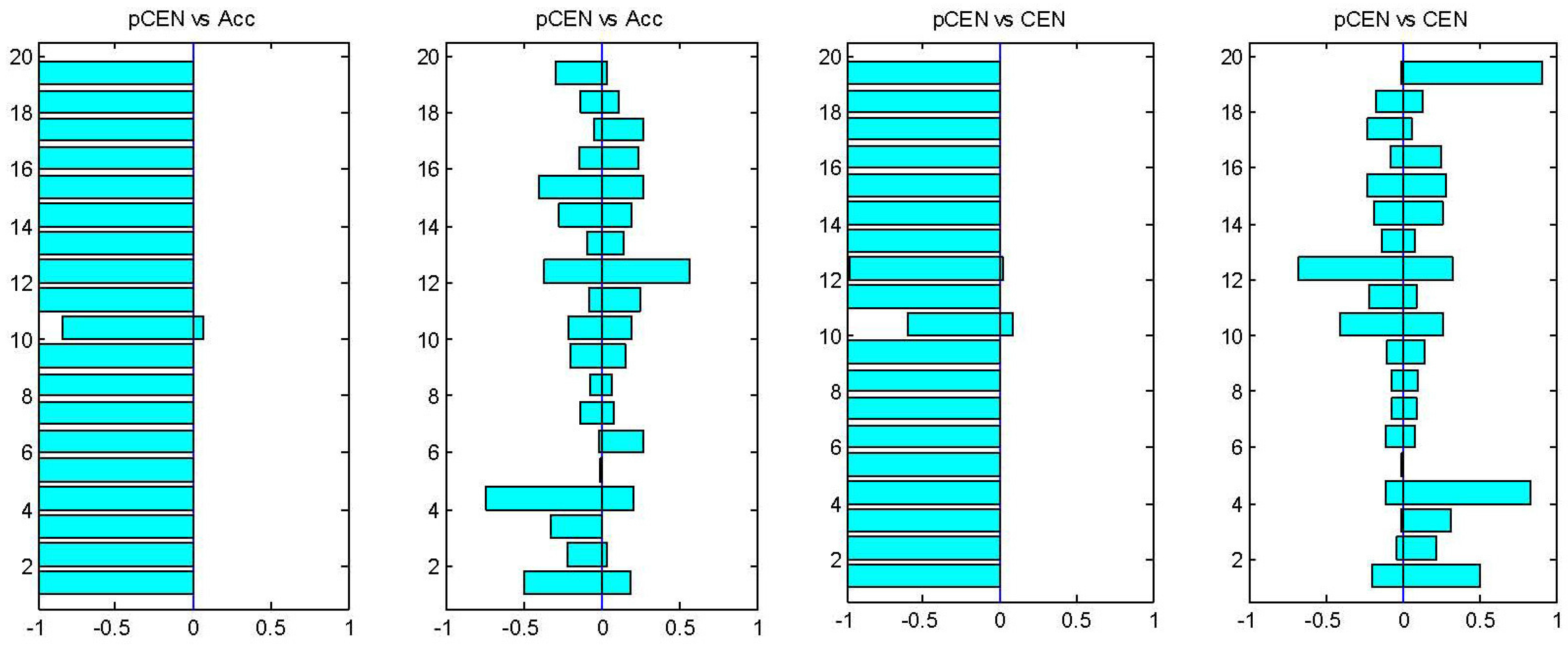
First of all, for simply showing the effectiveness of pCEN in comparison with the measures based on a threshold and a qualitative understanding of error, we simply present in Figure 1 the win-loss-equal statistics of pCEN vs. ACC and pCEN 
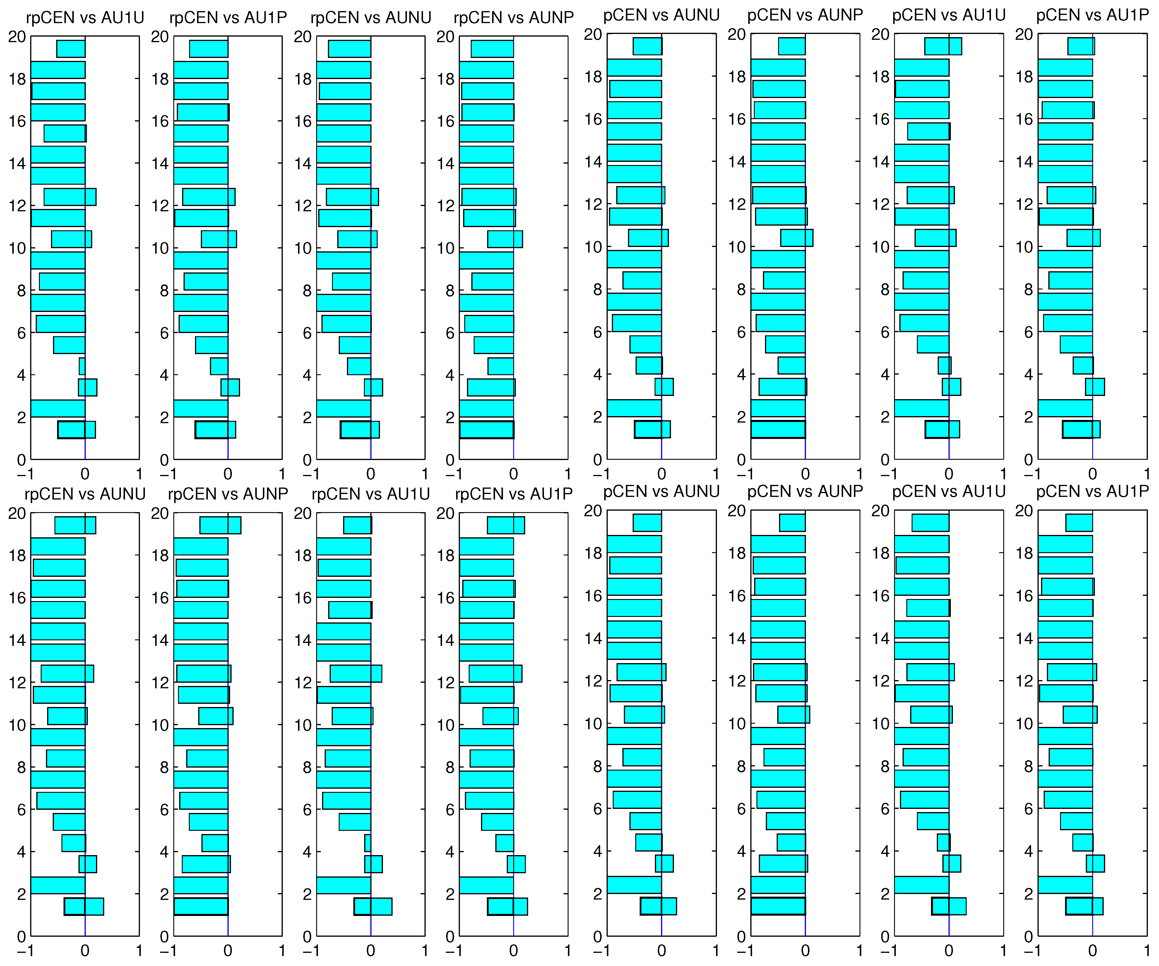
vs. CEN using pCEN, ACC and pCEN and CEN to choose the best classifiers. For comparing rpCEN and pCEN with the four variants of AUC, we present the win-loss-equal statistics using rpCEN and pCEN to choose the true best classifiers in Figure 2. From Figure 1, we can find that the probabilistic confusion entropy expectedly outperformed the accuracy and the confusion entropy on almost all of the datasets, which confirms the above discussion. From 
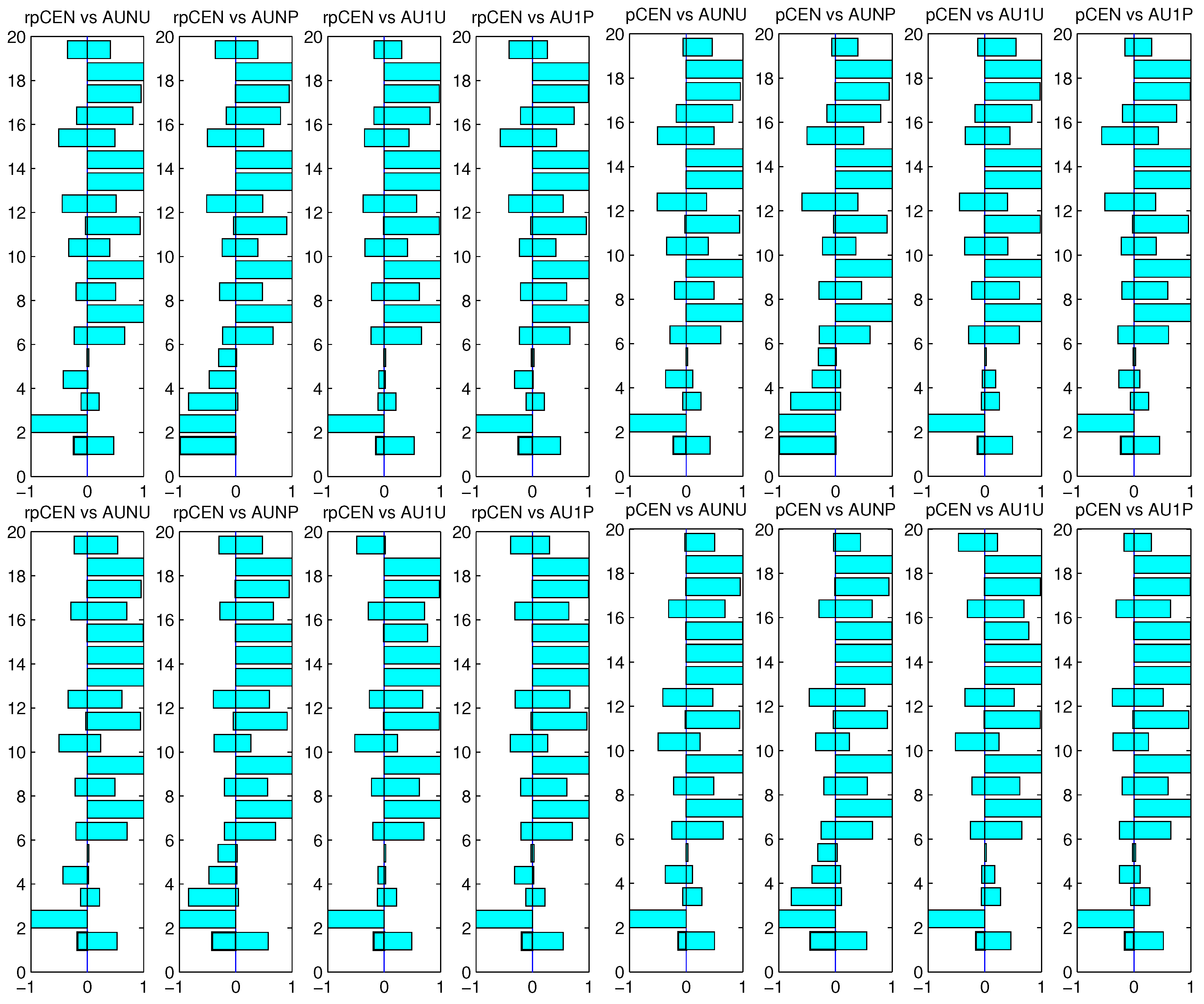
Figure 2, we can see that the relative probabilistic confusion entropy and probabilistic confusion entropy outperformed the four variants of AUC on almost all the datasets except for the third one. From
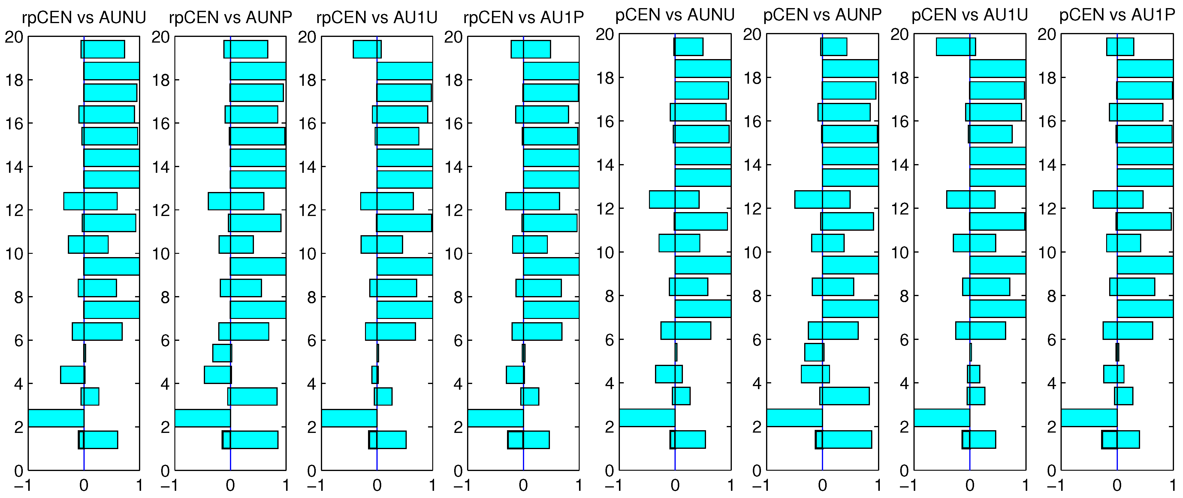
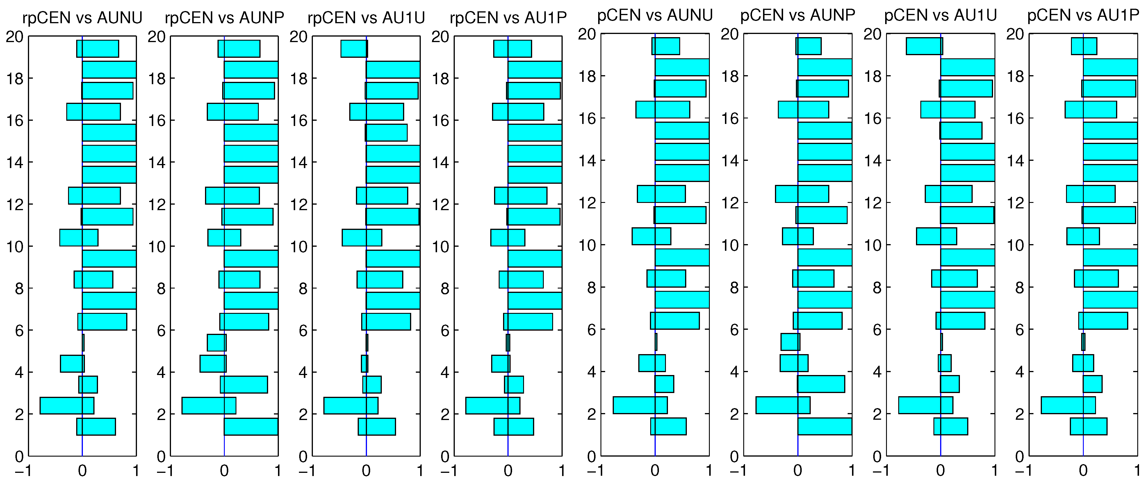
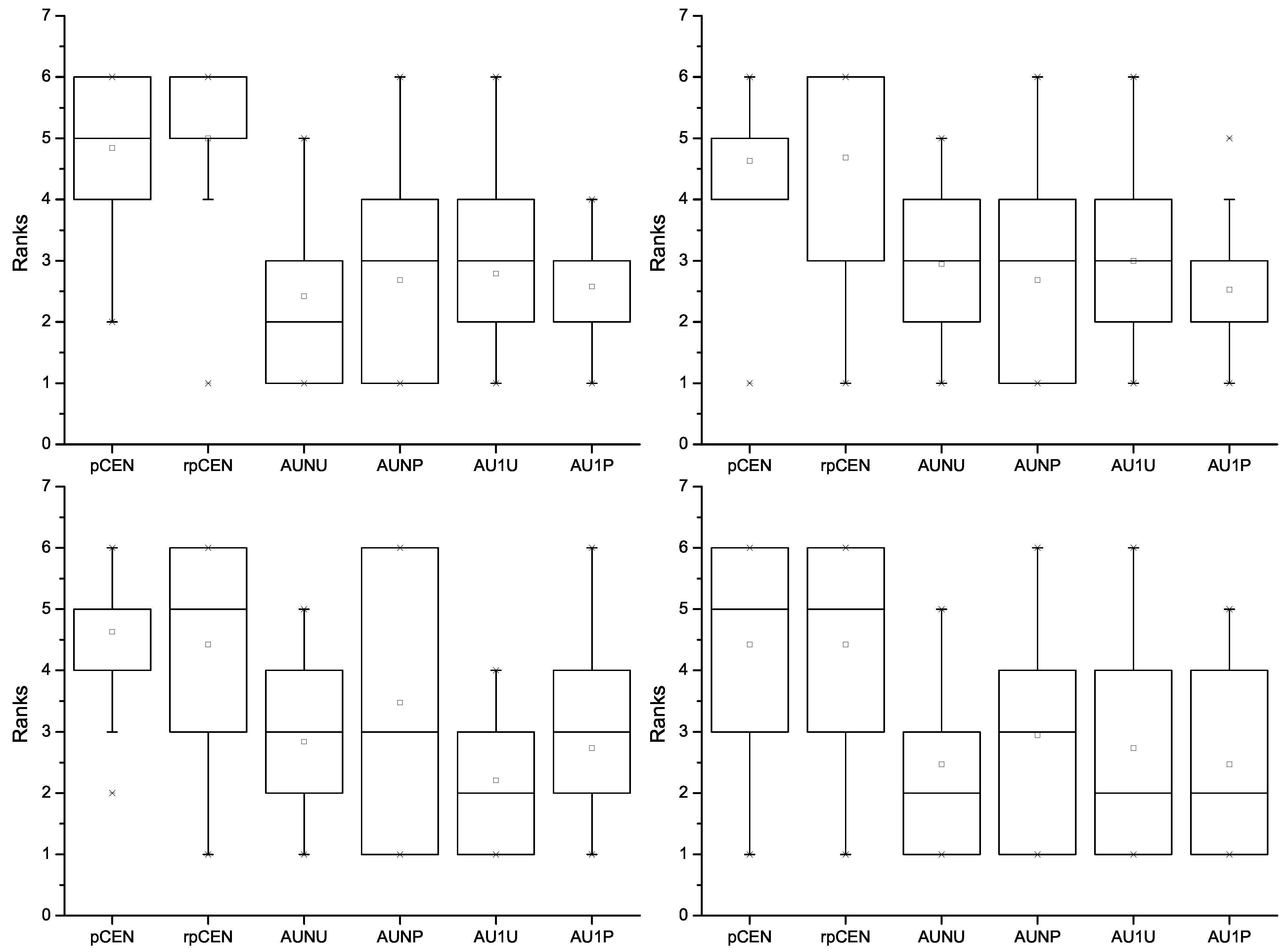
 Figure 3 and Figure 4, we can find that the four variants of AUC outperformed the two probabilistic confusion entropies on most of the datasets. The results shown in Figure 2, Figure 3 and Figure 4 obviously indicate that choosing the true best classifiers by a measure tends to rank the measure higher than the other measures. Nevertheless, as one may notice on some of the datasets, the four variants, when they were employed to choose the true best classifiers, did not appear to be as good as the two probabilistic confusion entropies, when the two measures were used to choose the true best classifiers. Hence, we can still determine that the two probabilistic confusion entropies are more effective than the four variants of AUC from the results shown in Figure 2, Figure 3 and Figure 4.
The win-loss-equal statistics using AUNU and AUNP to choose the true best classifiers are pictured in Figure 3. The win-loss-equal statistics using AU1U and AU1P to choose the true best classifiers are pictured in Figure 4
For further revealing how the compared measures performed, we calculated the average regrets of the 2,000 rounds for all the datasets. For each dataset, we ranked the six compared measures. The best was ranked the first and the worst the sixth. The rank results using rpCEN and pCEN to choose the true best classifiers are pictured in Figure 5. The rank results with respect to AUNU, AUNP, AU1U and AU1P are pictured in Figure 6.
Figure 1. Win-loss-equal statistics of pCEN vs. ACC (the left two) and pCEN vs. CEN (the right two). For each pair, the left figure corresponds to the results obtained using pCEN to choose the true best classifiers, the right corresponds to that using the compared measure.
Entropy 15 04969 g001
Figure 2. Win-loss-equal statistics of rpCEN, pCEN vs. AUNU, AUNP, AU1U and AU1P using rpCEN (the upper two) and pCEN (the lower two) to choose the true best classifiers.
Entropy 15 04969 g002
Figure 3. Win-loss-equal statistics of rpCEN, pCEN vs. AUNU, AUNP, AU1U and AU1P using AUNU (the upper two) and AUNP (the lower two) to choose the true best classifiers.
Entropy 15 04969 g003aEntropy 15 04969 g003b
Figure 4. Win-loss-equal statistics of rpCEN, pCEN vs. AUNU, AUNP, AU1U and AU1P using AU1U (the upper two) and AU1P (the lower two) to choose the true best classifiers.
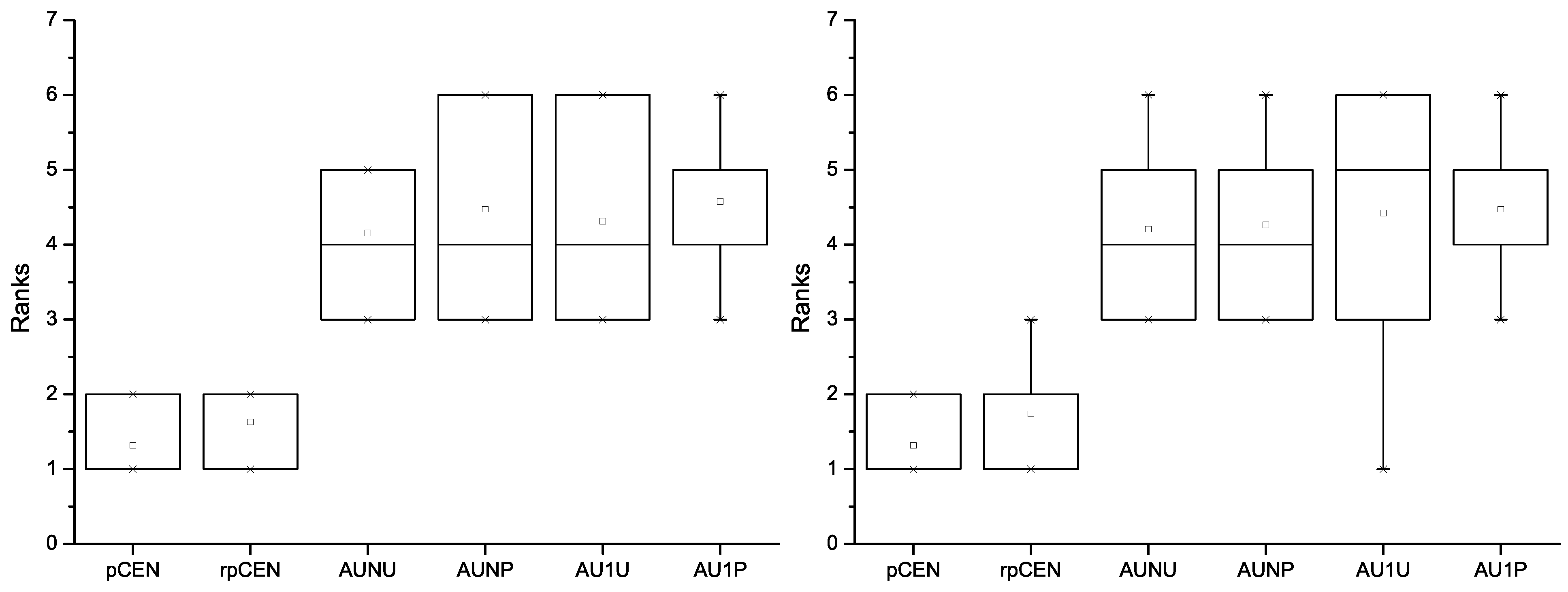
Entropy 15 04969 g004
Figure 5. The ranks of rpCEN, pCEN, AUNU, AUNP, AU1U and AU1P using rpCEN (the left) and pCEN (the right) to choose the true best classifiers.
Entropy 15 04969 g005
Figure 6. The ranks of rpCEN, pCEN, AUNU, AUNP, AU1U and AU1P using AUNU (the upper left), AUNP (the upper right), AU1U (the lower left) and AU1P (the lower right) to choose the true best classifiers.
Entropy 15 04969 g006
From Figure 5 and Figure 6, we can also find that the measures tended to be ranked higher when they were employed to choose the true best classifiers. Nevertheless, it is easy to find that the relative probabilistic confusion entropy and the probabilistic confusion entropy obviously outperformed the four variants of AUC. When rpCEN was used to choose the true best classifiers, no variant of AUC was ranked ahead of the two probabilistic confusion entropies on all datasets. Their average ranks turned out to be larger than 1 but smaller than 2. In comparison, though each variant of AUC was ranked higher on average than the other three variants and the two probabilistic confusion entropies when it was employed to choose the true best classifiers, all the other measures were ranked higher on some of the datasets. Besides, the average rank of each variant turned out to be larger than 2, even when it was employed to choose the true best classifiers.
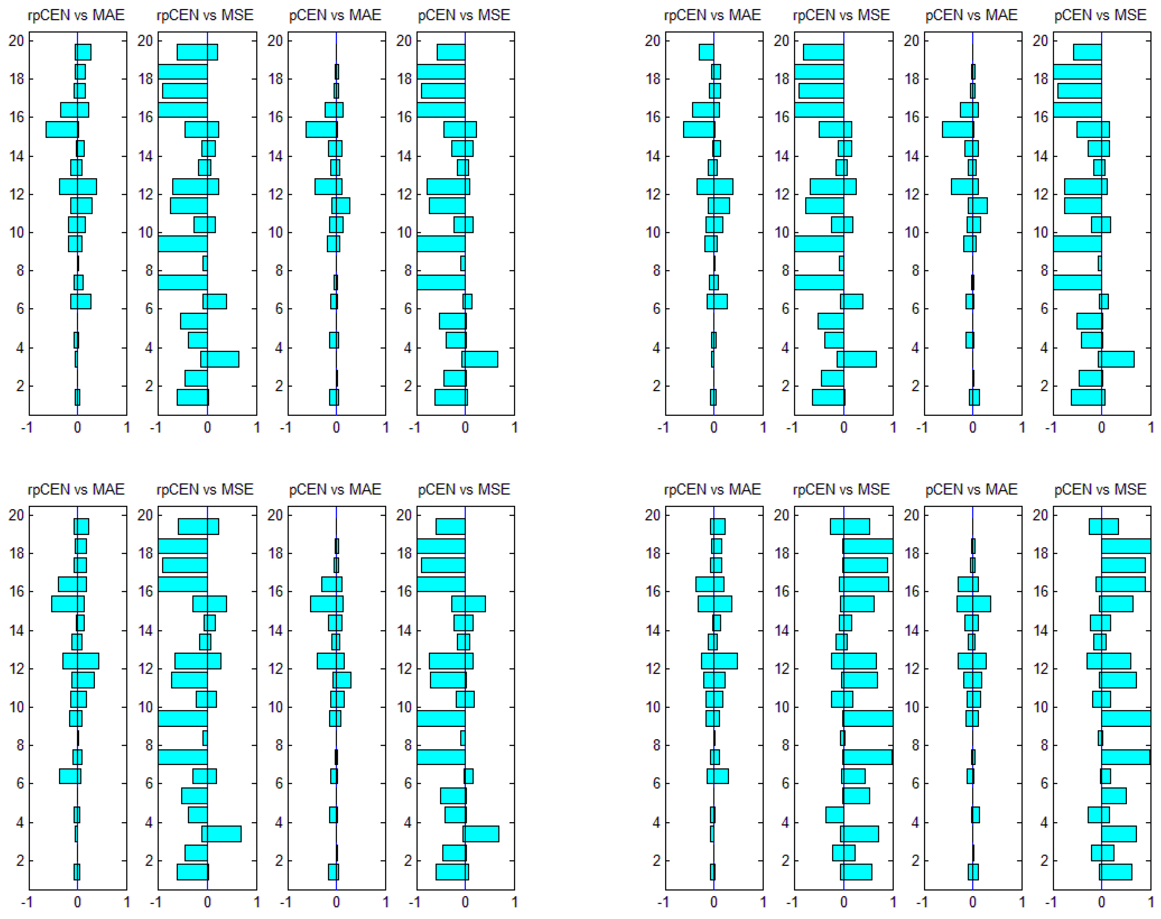
Figure 7. Win-loss-equal statistics of rpCEN and pCEN vs. MAE and MSE using pCEN (the upper left), rpCEN (the upper right), MAE (the lower left) and MSE (the lower right) to choose the true best classifiers.
Entropy 15 04969 g007
Experiments were similarly conducted to compare probabilistic confusion entropy with MAE and MSE. The win-loss-equal statistics of rpCEN, pCEN vs. MAE and MSE are shown in Figure 7. First of all, it can be noticed in Figure 7 that pCEN, rpCEN and MSE appear to be superior respectively when they were used to choose the true best classifiers, though pCEN and rpCEN appear to be a little bit more superior to MSE. In contrast to this result, pCEN and rpCEN appear to be similar to MAE when each of the four measures, including MSE, was used to choose the true best classifiers. Besides, pCEN and rpCEN appear to be superior to MSE when MAE is used to choose the true best classifiers. For further investigating the relation between pCEN and rpCEN and MSE and MAE, the rank results with respect to the four measures are pictured in 
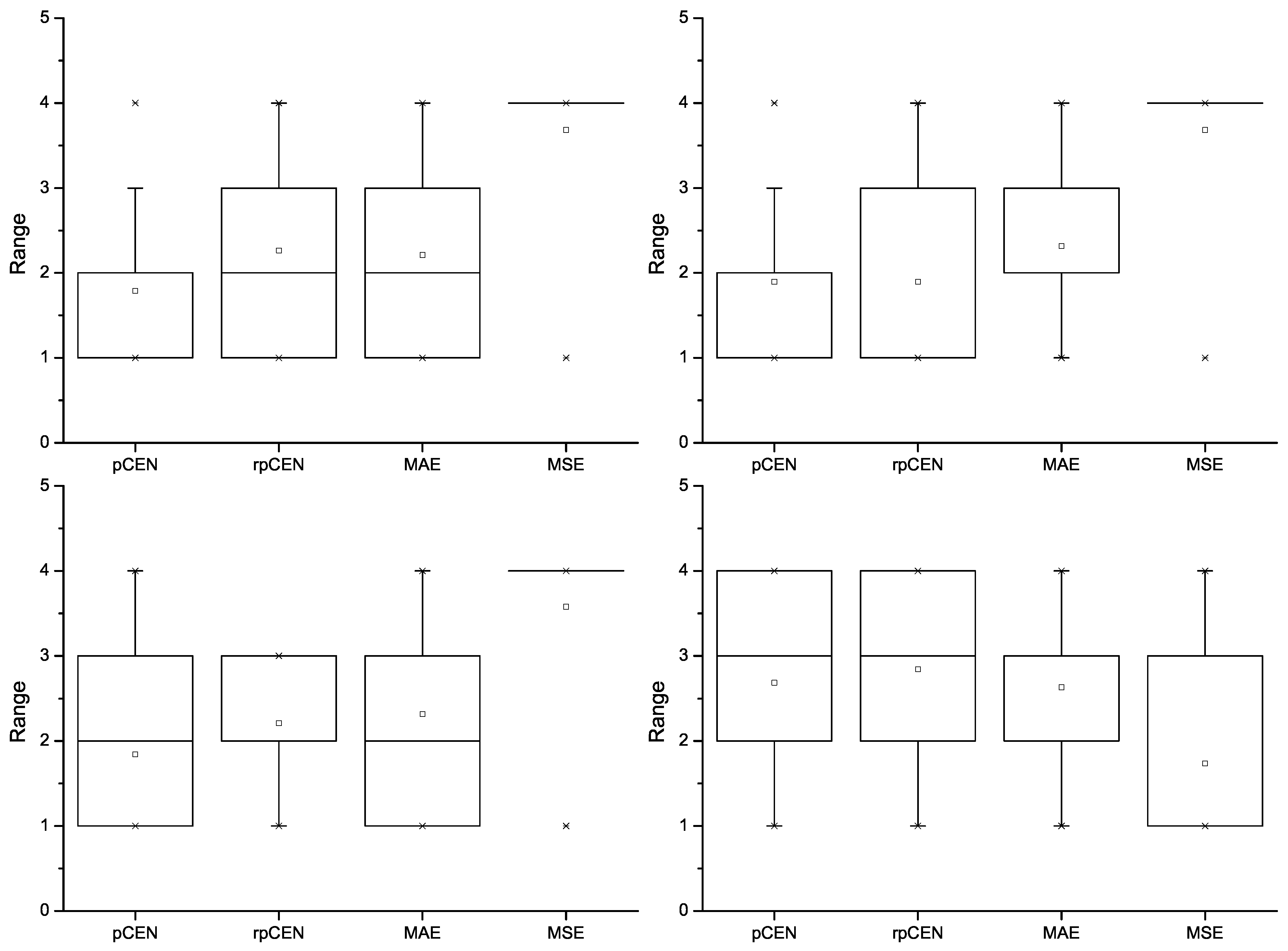
Figure 8. From the figure, it also can be seen that pCEN, rpCEN and MSE appear to be superior respectively when they were used to choose the best classifiers. Additionally, in comparison, pCEN and rpCEN appear to be superior to MSE, for they were not ranked higher than 3, even when MSE or MAE was used to choose the true best classifiers. MAE ranks pCEN and rpCEN higher than MSE. It is obvious to see that pCEN and rpCEN is superior to MAE, even when MAE was used to choose the true best classifiers.
Figure 8. The ranks of rpCEN, pCEN, MAE and MSE using pCEN (the upper left), rpCEN (the upper right), MAE (the lower left) and MSE (the lower right) to choose the true best classifiers.
Entropy 15 04969 g008
The results shown in Figure 5, Figure 6 and Figure 8 indicate that the improved confusion entropy was capable of evaluating classifiers consistently for different datasets. It is more stable than the compared measure. Hence, the improved probabilistic confusion entropy is more reliable for classifier evaluation. All the results show that the two probabilistic confusion entropies are effective for evaluating classifiers.

6. Conclusions

In this paper, the measure of confusion entropy is improved for evaluating classification models of information systems. For exploiting the probabilities of samples that are classified into different classes, we propose to compute the probabilities of one class samples classified into all classes and obtain a probabilistic confusion matrix. We then propose to compute confusion entropy based on a probabilistic confusion matrix. The simply improved measure still possesses the merit of taking into account both the classification accuracy and class discrimination power of classifiers. Furthermore, the improved measure can also be expected to differentiate whether or not samples are classified into true classes and are separated from other classes with high probabilities. Mathematical analysis shows that the improved measure is superior to the measures based on a threshold and a qualitative understanding of error. The analysis also shows that most measures based on a probabilistic understanding of error, e.g., macro average mean probability rate, mean probability rate, mean absolute error, LogLoss, etc., are incapable of evaluating the class discrimination power of classifiers. Finally, the experimental results on 19 benchmark datasets show that the improved measure is more effective than the four variants of AUC, MAE and MSE. Furthermore, the results also show that the improved measure does not stand or fall over different datasets.

Acknowledgments

This work was supported by the National Natural Science Foundation of China under grant 61070089, the Science Foundation of Tianjin under grant 10JCZDJC15800, 13ZCZDGX02200 and the Doctor Foundation of Tianjin Normal University under grant 52XB1101.

Conflict of Interest

The authors declare no conflict of interest.

References

  1. Egan, J.P. Signal Detection Theory and ROC Analysis. In Series in Cognition and Perception; Academic Press: New York, NY, USA, 1975. [Google Scholar]
  2. Spackman, K.A. Signal Detection Theory: Valuable Tools for Evaluating Inductive Learning. In Proceedings of the 6th International Workshop on Machine Learning, Ithaca, NY, USA, 26–27 June 1989; pp. 160–163.
  3. Wei, J.M.; Yuan, X.J.; Hu, Q.H.; Wang, S.Q. A novel measure for evaluating classifiers. Expert Syst. Appl. 2010, 37, 3799–3809. [Google Scholar] [CrossRef]
  4. Jurman, G.; Riccadonna, S.; Furlanello, C. A comparison of MCC and CEN error measures in multi- class prediction. PLoS One 2012, 7, 1–8. [Google Scholar] [CrossRef] [PubMed]
  5. Ferri, C.; Hernández-Orallo, J.; Modroiu, R. An experimental comparison of performance measures for classification. Pattern Recognit. Lett. 2009, 30, 27–38. [Google Scholar] [CrossRef]
  6. Forbes, A.D. Classification-algorithm evaluation: five performance measures based on confusion matrices. J. Clin. Monit. 1995, 11, 189–206. [Google Scholar] [CrossRef] [PubMed]
  7. Youden, W.J. Index for rating diagnostic tests. Cancer 1950, 3, 32–35. [Google Scholar] [CrossRef]
  8. Fluss, R.; Faraggi, D.; Reiser, B. Estimation of the Youden Index and it’s associated cutoff point. Biom. J. 2005, 47, 458–472. [Google Scholar] [CrossRef] [PubMed]
  9. Blakeley, D.; Oddone, E.; Hasselblad, V.; Simel, D.; Matchar, D. Noninvasive carotid artery testing: A meta-analytic review. Ann. Intern. Med. 1995, 122, 360–367. [Google Scholar] [CrossRef] [PubMed]
  10. Cohen, J. A coefficient of agreement for nominal scales. Educ. Psychol. Meas. 1960, 20, 37–46. [Google Scholar] [CrossRef]
  11. Fleiss, J.L. Statistical Methods for Rates and Proportions, 2nd ed.; Wiley: New York, NY, USA; Chichester, UK, 1981. [Google Scholar]
  12. Sindhwani, V.; Bhattacharya, P.; Rakshit, S. Information Theoretic Feature Crediting in Multiclass Support Vector Machines. In Proceedings of the First SIAM International Conference on Data Mining (ICDM’01), Chicago, IL, USA, 5–7 April 2001; pp. 5–7.
  13. Statnikov, A.; Aliferis, C.F.; Tsamardinos, I.; Hardin, D.; Levy, S. A comprehensive evaluation of multicategory classification methods for microarray gene expression cancer diagnosis. Bioinformatics 2005, 21, 631–643. [Google Scholar] [CrossRef] [PubMed]
  14. Wickens, T.D. Multiway Contingency Table Analysis for the Social Sciences; Lawrence Erlbaum: Hillsdale, NJ, USA, 1989. [Google Scholar]
  15. Gorodkin, J. Comparing two K-category assignments by a K-category correlation coefficient. Comput. Biol. Chem. 2004, 28, 367–74. [Google Scholar] [CrossRef] [PubMed]
  16. Yates, R.B.; Neto, B.R. Modern Information Retrieval; Addison Wesley: New York, NY, USA, 1999. [Google Scholar]
  17. Mitchell, T.M. Machine Learning; McGraw-Hill: New York, NY, USA, 1997. [Google Scholar]
  18. Lebanon, G.; Lafferty, J. Cranking: Combining Rankings Using Conditional Probability Models on Permutations. In Proceedings of the 19th International Conference (ICML 2002), Sydney, Australia, 8–12 July 2002; pp. 363–370.
  19. Good, I.J. Rational decisions. J. R. Stat. Soc. Series B 1952, 14, 107–114. [Google Scholar]
  20. Good, I.J. Corroboration, explanation, evolving probability, simplicity, and a sharpened razor. Br. J. Philos. Sci. 1968, 19, 123–143. [Google Scholar] [CrossRef]
  21. Fawcett, T.; Niculescu-Mizil, A. PAV and the ROC convex hull. Mach. Learn. 2007, 68, 97–106. [Google Scholar] [CrossRef]
  22. Flach, P.; Matsubara, E.T. A Simple Lexicographic Ranker and Probability Estimator. In Proceedings of the 18th European Conference on Machine Learning, Warsaw, Poland, 17–21 September 2007; pp. 575–582.
  23. Caruana, R.; Niculescu-Mizil, A. Data Mining in Metric Space: An Empirical Analysis of Supervised Learning Performance Criteria. In Proceedings of the 10th ACM SIGKDD International Conference on Knowledge Discovery and Data Mining (KDD’04), Seattle, WA, USA, 22–25 August 2004; pp. 69–78.
  24. Fawcett, T. An introduction to ROC analysis. Pattern Recognit. Lett. 2006, 27, 861–874. [Google Scholar] [CrossRef]
  25. Bradley, A.P. The use of the area under the ROC curve in the evaluation of machine learning algorithms. Pattern Recognit. 1997, 30, 1145–1159. [Google Scholar] [CrossRef]
  26. Landgrebe, T.C.W.; Duin, R.P.W. Efficient multiclass ROC approximation by decomposition via confusion matrix perturbation analysis. IEEE Trans. Pattern Anal. Mach. Intell. 2008, 30, 810–822. [Google Scholar] [CrossRef] [PubMed]
  27. Hand, D.J. Measuring classifier performance: A coherent alternative to the area under the ROC curve. Mach. Learn. 2009, 77, 103–123. [Google Scholar] [CrossRef]
  28. Hand, D.J. Evaluating diagnostic tests: the area under the ROC curve and the balance of errors. Stat. Med. 2010, 29, 1502–1510. [Google Scholar] [CrossRef] [PubMed]
  29. Flach, P.; Hernández-Orallo, J.; Ferri, C. A Coherent interpretation of AUC as a measure of aggregated classification performance. In Proceedings of the 28th International Conference on Machine Learning (ICML’11), Bellevue, WA, USA, 28 June–2 July 2011; pp. 657–664.
  30. Fawcett, T. Using Rule Sets to Maximize ROC Performance. In Proceedings of the 2001 IEEE International Conference on Data Mining (ICDM-01), San Jose, CA, USA, 29 November–2 December 2001; p. 131.
  31. Hand, D.J.; Till, R.J. A simple generalisation of the area under the ROC curve for multiple class classification problems. Mach. Learn. 2001, 45, 171–186. [Google Scholar] [CrossRef]
  32. Wu, S.; Flach, P.; Ferri, C. An Improved Model Selection Heuristic for AUC. In Proceedings of the 18th European Conference on Machine Learning, Warsaw, Poland, 17–21 September 2007; pp. 478–489.
  33. Ferri, C.; Flach, P.; Hernández-Orallo, J.; Senad, A. Modifying ROC Curves to Incorporate Predicted Probabilities. In Proceedings of the ICML 2005 Workshop on ROC Analysis in Machine Learning, Bonn, Germany, 7–11 August 2005; pp. 33–40.
  34. Provost, F.; Fawcett, T. Analysis and Visualization of Classifier Performance: Comparison Under Imprecise Class and Cost Distributions. In Proceedings of the Third International Conference on Knowledge Discovery and Data Mining, Newport Beach, CA, USA, 14–17 August 1997; pp. 43–48.
  35. Provost, F.; Fawcett, T. Robust classification for imprecise environments. Mach. Learn. 2001, 42, 203–231. [Google Scholar] [CrossRef]
  36. Drummond, C.; Holte, R.C. Cost curves: An improved method for visualizing classifier performance. Mach. Learn. 2006, 65, 95–130. [Google Scholar] [CrossRef]
  37. Japkowicz, N.; Sanghi, P.; Tischer, P. A projection-based framework for classifier performance evaluation. Lecture Notes Comput. Sci. 2008, 5211, 548–563. [Google Scholar]
  38. Hernández-Orallo, J.; Flach, P.; Ferri, C. Brier Curves: A New Cost-Based Visualisation of Classifier Performance. In Proceedings of the 28th International Conference on Machine Learning, Bellevue, WA, USA, 28 June–2 July 2011; pp. 585–592.
  39. Metz, C. Basic principles of ROC analysis. Semin. Nucl. Med. 1978, 8, 283–298. [Google Scholar] [CrossRef]
  40. Hanley, J.A.; McNeil, B.J. The meaning and use of the area under a receiver operating characteristics(ROC) curve. Radiology 1983, 148, 29–36. [Google Scholar] [CrossRef] [PubMed]
  41. Swets, J. Measuring the accuracy of diagnostic systems. Scince 1988, 240, 1285–1293. [Google Scholar] [CrossRef]
  42. Drummond, C. Machine Learning as an Experimental Science (Revisited). In Proceedings of the AAAI06-Workshop on Evaluation Methods for Machine Learning, Boston, MA, USA, 16–20 July 2006.
  43. Hand, D.J. Construction and Assessment of Classification Rules; John Wiley and Sons: New York, NY, USA, 1997. [Google Scholar]
  44. Hand, D.J. Measuring diagnostic accuracy of statistical prediction rules. Stat. Neerlandica 2001, 55, 3–16. [Google Scholar] [CrossRef]
  45. Sokolova, M.; Japkowicz, N.; Szpakowicz, S. Beyond accuracy, F-score and ROC: A family of discriminant measures for performance evaluation. AI 2006, Lecture Notes Comput. Sci. 2006, 4304, 1015–1021. [Google Scholar]
  46. Sokolova, M.; Lapalme, G. A systematic analysis of performance measures for classification tasks. Inf. Process. Manag. 2009, 45, 427–437. [Google Scholar] [CrossRef]
  47. Bishop, C.M. Neural Networks for Pattern Recognition; Oxford University Press: Oxford, UK, 1995. [Google Scholar]
  48. Harrell, F.E., Jr. Regression Modeling Strategies: With Applications to Linear Models, Logistics Regression, and Survival Analysis; Springer: Berlin/Heidelberg, Germany, 2001. [Google Scholar]
  49. Ripley, B.D. Pattern Recognition and Neural Networks; Cambridge University Press: Cambridge, UK, 1996. [Google Scholar]
  50. Hernández-Orallo, J.; Flach, P.; Ferri, C. A unified view of performance metrics: Translating threshold choice into expected classification loss. J. Mach. Learn. Res. 2012, 13, 2813–2869. [Google Scholar]
  51. Gu, Q.; Zhu, L.; Cai, Z. Evaluation Measures of the Classification Performance of Imbalanced datasets. In Computational Intelligence and Intelligent Systems, Proceedings of the 4th International Symposium on Intelligence Computation and Applications (ISICA 2009), Huangshi, China, 23–25 October 2009; Springer: Huangshi, China, 2009; Volume 51, pp. 461–471. [Google Scholar]
  52. Labatut, V.; Cherifi, H. Evaluation of performance measures for classifiers comparison. Ubiquitous Comput. Commun. J. 2011, 6, 21–34. [Google Scholar]
  53. Huang, J.; Ling, C. Constructing New and Better Evaluation Measures for Machine Learning. In Proceedings of the 20th International Joint Conference on Artificial Intelligence (IJCAI’2007), Hyderabad, India, 9–12 January 2007; pp. 859–864.
  54. Witten, I.H.; Frank, E. Data Mining: Practical Machine Learning Tools and Techniques, 2nd ed.; Morgan Kaufmann: San Francisco, CA, USA, 2005. [Google Scholar]
  55. Vanderlooy, S.; Hüllermeier, E. A critical analysis of variants of the AUC. Mach. Learn. 2008, 72, 247–262. [Google Scholar] [CrossRef]
  56. Brier, G.W. Verification of forecasts expressed in terms of probability. Mon. Weather Rev. 1950, 78, 1–3. [Google Scholar] [CrossRef]
  57. UCI Machine Learning. Available online: http://mlearn/MLRepository.html (accessed on 4 November 2013).
  58. Quinlan, J.R. C4.5: Programs for Machine Learning; Morgan Kaufmann: San Mateo, CA, USA, 1993. [Google Scholar]

