Article

Analysis and Visualization of Seismic Data Using Mutual Information

by
José A. Tenreiro Machado
1,* and
António M. Lopes
2
1
Institute of Engineering, Polytechnic of Porto, Rua Dr. António Bernardino de Almeida, 431, Porto 4200-072, Portugal
2
Institute of Mechanical Engineering, Faculty of Engineering, University of Porto, Rua Dr. Roberto Frias, Porto 4200-465, Portugal
*
Author to whom correspondence should be addressed.
Entropy 2013, 15(9), 3892-3909; https://0-doi-org.brum.beds.ac.uk/10.3390/e15093892
Submission received: 26 July 2013 / Revised: 10 September 2013 / Accepted: 12 September 2013 / Published: 16 September 2013
(This article belongs to the Special Issue Dynamical Systems)

Abstract

:
Seismic data is difficult to analyze and classical mathematical tools reveal strong limitations in exposing hidden relationships between earthquakes. In this paper, we study earthquake phenomena in the perspective of complex systems. Global seismic data, covering the period from 1962 up to 2011 is analyzed. The events, characterized by their magnitude, geographic location and time of occurrence, are divided into groups, either according to the Flinn-Engdahl (F-E) seismic regions of Earth or using a rectangular grid based in latitude and longitude coordinates. Two methods of analysis are considered and compared in this study. In a first method, the distributions of magnitudes are approximated by Gutenberg-Richter (G-R) distributions and the parameters used to reveal the relationships among regions. In the second method, the mutual information is calculated and adopted as a measure of similarity between regions. In both cases, using clustering analysis, visualization maps are generated, providing an intuitive and useful representation of the complex relationships that are present among seismic data. Such relationships might not be perceived on classical geographic maps. Therefore, the generated charts are a valid alternative to other visualization tools, for understanding the global behavior of earthquakes.

1. Introduction

Earthquakes are caused by a sudden release of elastic strain energy accumulated between the surfaces of tectonic plates. Big earthquakes often manifest by ground shaking and can trigger tsunamis, landslides and volcanic activity. When affecting urban areas, earthquakes usually cause destruction and casualties [1,2,3,4]. Better understanding earthquake behavior can help to delineate pre-disaster policies, saving human lives and mitigating the economic efforts involved in assembling emergency teams, gathering medical and food supplies and rebuilding the affected areas [5,6,7,8].
Earthquakes reveal self-similarity and absence of characteristic length-scale in magnitude, space and time, caused by the complex dynamics of Earth’s tectonic plates [9,10]. The plates meet each other at fault zones, exhibiting friction and stick-slip behavior when moving along the fault surfaces [11,12]. The irregularities on the fault surfaces resemble rigid body fractals sliding over each other, originating the fractal scaling behavior observed in earthquakes [13]. The tectonic plates form a complex system due to interactions among faults, where motion and strain accumulation processes interact on different scales ranging from a few millimeters to thousands of kilometers [14,15,16]. Moreover, loading rates are not uniform in time. Earthquakes are likely to come in clusters, meaning that a cluster is most probable to occur shortly after another cluster and a cluster of clusters soon after another cluster of clusters [17]. Earthquakes unveil long range correlations and long memory characteristics [18], which are typical of fractional order systems [19,20]. Some authors also suggest that Self-Organized Criticality (SOC) is relevant for understanding earthquakes as a relaxation mechanism that organizes the terrestrial crust at both spatial and temporal levels [21]. Other researchers [22,23] emphasize the relationships between complex systems, fractals and fractional calculus [24,25,26,27].
In this paper, we analyze seismic data in the perspective of complex systems. Such data is difficult to analyze using classical mathematical tools, which reveal strong limitations in exposing hidden relationships between earthquakes. In our approach global data is collected from the Bulletin of the International Seismological Centre [28] and the period from 1962 up to 2011 is considered. The events, characterized by their magnitude, geographic location and time, are divided into groups, either according to the Flinn-Engdahl (F-E) seismic regions of Earth or using a rectangular grid based on latitude and longitude coordinates. We develop and compare two alternative approaches. In a first methodology, the distributions of magnitudes are approximated by Gutenberg-Richter (G-R) distributions and the corresponding parameters are used to reveal the relationships among regions. In the second approach, the mutual information is adopted as a measure of similarity between events in the distinct regions. In both cases, clustering analysis and visualization maps are adopted as an intuitive and useful representation of the complex relationships among seismic events. The generated maps are evidenced as a valid alternative to standard visualization tools, for understanding the global behavior of earthquakes.
Bearing these ideas in mind, this paper is organized as follows: in Section 2, we give a brief review of the techniques used. Section 3 analyses earthquakes’ data and discusses results, adopting F-E seismic regions. Section 4 extends the analysis to an alternative seismic regionalization of Earth. Finally, Section 5 outlines the main conclusions.

2. Mathematical tools

This section presents the main mathematical tools adopted in this study, namely G-R distributions, mutual information and clustering analysis. The G-R distribution is a two-parameter power-law (PL) that establishes a relationship between frequency and magnitude of earthquakes [29,30,31].
The concepts of entropy and mutual information [32,33,34,35], taken from the information theory, have been a common approach to the analysis of complex systems [36]. In particular, mutual information is adopted as a general measure of correlation between two systems. Mutual information, as well as entropy, have found significance in various applications in diverse fields, such as in analyzing experimental time series [37,38,39], in characterizing symbol sequences such as DNA sequences [40,41,42] and in providing a theoretical basis for the notion of complexity [43,44,45,46,47], just to name a few.
Clustering analysis consists on grouping objects in such a way that objects that are, in some sense, similar to each other are placed in the same group (cluster). Clustering is a common technique for statistical data analysis, used in many fields, such as data mining, machine learning, pattern recognition, image analysis, information retrieval and bioinformatics [48,49,50].

2.1. Gutenberg-Richter Law

The G-R law is given by:
log 10 N = a b M
where NN is the number of earthquakes of magnitude greater than or equal to MR, occurred in a specified region and period of time. Parameters (a, b) ∈ R represent the activity level and the scaling exponent, respectively. The former is a measure of the level of seismicity, being related to the number of occurrences. The later has regional variation, being in the range b ∈ [0.8, 1.06] and b ∈ [1.23, 1.54] for small and big earthquakes, respectively [30].

2.2. Mutual Information

Mutual information measures the statistical dependence between two random variables. In other words, it gives the amount of information that one variable “contains” about the other. Let X and Y represent two discrete random variables with alphabet X and Y, respectively. The mutual information between X and Y, I(X, Y), is given by [51]:
I ( X , Y ) = y Y x X p ( x , y ) log 2 ( p ( x , y ) p ( x ) p ( x ) )
where p(x, y) is the joint probability distribution function of (X, Y), and p(x) and p(y) are the marginal probability distribution functions of X and Y, respectively. Mutual information is always symmetrical (i.e., I(X, Y) = I(Y, X)). If the two variables are independent, the mutual information is zero.

2.3. K-means Clustering

K-means is a popular non-hierarchical clustering method, extensively used in machine learning and data mining. K-means starts with a collection of N objects XN ={x1, x2, …, xN}, where each object xn (1 ≤ n < N) is a point in D-dimensional space (xnRD), and a user specified number of clusters, K. The K-means method aims to partition the N objects into KN clusters, CK = {c1, c2, …, cK}, so as to minimize the sum of distances, J, between the points and the centers of their clusters, MK = {µ1, µ2, …, µK}:
J = n = 1 N k = 1 K r n k x n μ k 2
where rnk ∈ {0, 1} is a parameter denoting whether object xn belongs to cluster k [52]. The result can be seen as partitioning the data space into K Voronoi cells.
The exact optimization of the K-means objective function, J, is NP-hard. Several efficient heuristic algorithms are commonly used, aiming to converge quickly to local minima. Among others [53] Lloyd’s algorithm, described in the sequel, is one of the most popular. It initializes computing the cluster centers MK = {µ1, µ2, …, µK}. This can is done randomly choosing the centers, adopting K objects as the cluster centers, or using other heuristics. After initialization, the algorithm iterates assigning each object to its closest cluster center:
c k = { n : k = arg min k x n μ k 2 }
where ck represents the set of objects closest to µk.
New cluster centers, μk, are then calculated using:
μ k = 1 | c k | n c k x n
and Equations (4) and (5) are repeated until some criterion is met (e.g., cluster centers do not change in space anymore).
One way to select the appropriate number of clusters, K, for the K-means algorithm is plotting the K-means objective, J, versus K, and looking at the “elbow” of the curve. The “optimum” value for K corresponds to the point of maximum curvature.

2.4. Hierarchical Clustering

Hierarchical clustering aims to build a hierarchy of clusters [54,55,56,57]. In agglomerative clustering each object starts in its own singleton cluster and, at each step, the two most similar (in some sense) clusters are greedily merged. The algorithm iterates until there is a single cluster containing all objects. In divisive clustering, all objects start in one single cluster. At each step, the algorithm removes the “outsiders” from the least cohesive cluster, stopping when each object is in its own singleton cluster. The results of hierarchical clustering are usually presented in the form of a dendrogram.
The clusters are combined (for agglomerative), or split (for divisive) based on a measure of dissimilarity between clusters. This is often achieved by using an appropriate metric (a measure of the distance between pairs of objects) and a linkage criterion, which defines the dissimilarity between clusters as a function of the pairwise distances between objects. The chosen metric will influence the composition of the clusters, as some elements may be closer to one another, according to one metric, and farther away, according to another.
Given two clusters, R and S, any metric can be used to measure the distance, d(xR, xS), between objects (xR, xS). The Euclidean and Manhattan distances are often adopted. Based on these metrics, the maximum, minimum and average linkages are commonly used, being, respectively:
d max ( R , S ) = max x R R , x S S d ( x R , x S )
d min ( R , S ) = min x R R , x S S d ( x R , x S )
d a v e ( R , S ) = 1 | R | | S | x R R , x S S d ( x R , x S )
While non-hierarchical clustering produces a single partitioning of K clusters, hierarchical clustering can give different partitioning spaces, depending on the chosen distance threshold.

3. Analysis Global Seismic Data

The Bulletin of the International Seismological Centre (ISC) [28] is adopted in what follows. The ISC Bulletin contains seismic events since 1904, contributed by more than 17,000 seismic stations located worldwide. Each data record contains information about magnitude, geographic location and time. Occurrences with magnitude in the interval M ∈ [–2.1, 9.2], expressed in a logarithm scale consistent with the local magnitude or Richter scale, are available [28]. In the first period of registers (about half a century) the number of records is remarkable smaller and lower magnitude events are scarce, when compared to the most recent fifty years. This may be justified by the technological constraints associated to the instrumentation available in the early decades of the last century. Therefore, to prevent misleading results, we study the fifty-year period from 1962 up to 2011. The events are divided into the fifty groups corresponding to the Flinn-Engdahl (F-E) regions of Earth [58,59], which correspond to seismic zones usually used by seismologists for localizing earthquakes (Table 1).
Table 1. Flinn-Engdahl regions of Earth and characterization of the seismic data.
Region numberRegion nameNumber of eventsMinimum MagnitudeMaximum MagnitudeAverage Magnitude
1Alaska-Aleutan arc38,9760.98.03.7
2Southeastern Alaska to Washington19,3890.37.12.6
3Oregon, California and Nevada26,1880.07.62.9
4Baja California and Gulf of California7,6211.17.22.7
5Mexico-Guatemala area29,9911.97.93.9
6Central America20,5240.07.53.8
7Caribbean loop48,5920.77.33.0
8Andean South America81,2091.28.53.5
9Extreme South America2,5440.06.33.2
10Southern Antilles6,1020.37.54.4
11New Zealand region58,270−0.18.13.2
12Kermadec-Tonga-Samoa Basin area50,1291.78.14.1
13Fiji Islands area23,7231.07.24.0
14Vanuatu Islands29,062−1.47.94.1
15Bismarck and Solomon Islands29,600−1.48.04.0
16New Guinea24,991−0.27.84.0
17Caroline Islands area5,0160.07.04.1
18Guam to Japan33,9981.27.53.7
19Japan-Kuril Islands-Kamchatka Peninsula865,5790.08.31.6
20Southwestern Japan and Ryukyu Islands583,9920.17.41.1
21Taiwan area285,357−0.87.92.2
22Philippine Islands31,2770.08.43.9
23Borneo-Sulawesi34,2790.07.54.0
24Sunda arc46,4300.08.44.0
25Myanmar and Southeast Asia7,8530.07.43.1
26India-Xizang-Sichuan-Yunnan29,361−0.68.02.7
27Southern Xinjiang to Gansu15,4640.08.02.9
28Lake Issyk-Kul to Lake Baykal32,3301.37.42.6
29Western Asia21,6210.08.13.2
30Middle East-Crimea-Eastern Balkans220,6073.18.42.7
31Western Mediterranean area194,094−0.57.21.9
32Atlantic Ocean37,502−0.37.02.8
33Indian Ocean12,8480.07.74.1
34Eastern North America15,104−2.17.32.7
35Eastern South America670.05.74.3
36Northwestern Europe91,1900.05.91.6
37Africa49,3700.07.42.5
38Australia7,7592.26.52.5
39Pacific Basin3,0032.37.02.9
40Arctic zone18,7862.16.92.4
41Eastern Asia13,7901.67.82.6
42Northeast. Asia, North. Alaska to Greenland6,8231.87.63.1
43Southeastern and Antarctic Pacific Ocean6,9430.07.14.3
44Galápagos Islands area2,351−0.66.44.2
45Macquarie loop1,7432.27.84.3
46Andaman Islands to Sumatera20,7620.99.24.0
47Baluchistan4,1010.37.63.9
48Hindu Kush and Pamir area39,6690.07.33.0
49Northern Eurasia60,0821.15.91.4
50Antarctica641.95.54.0

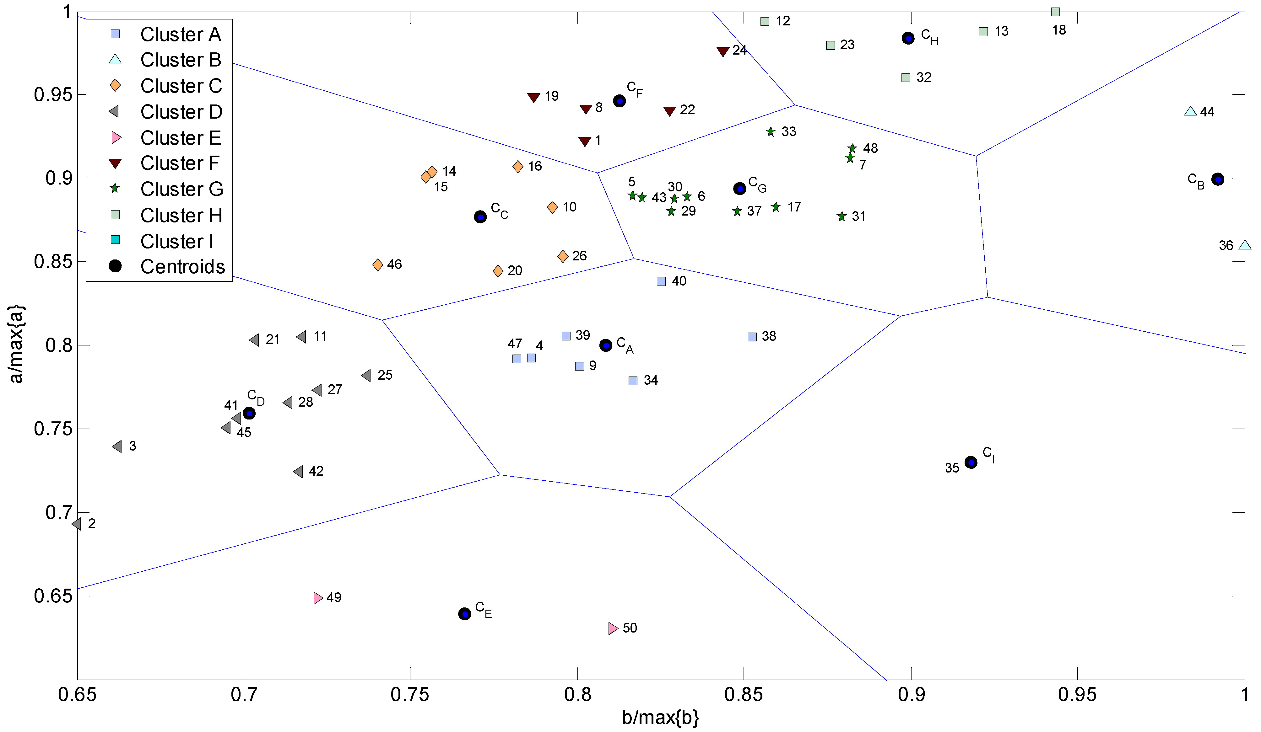
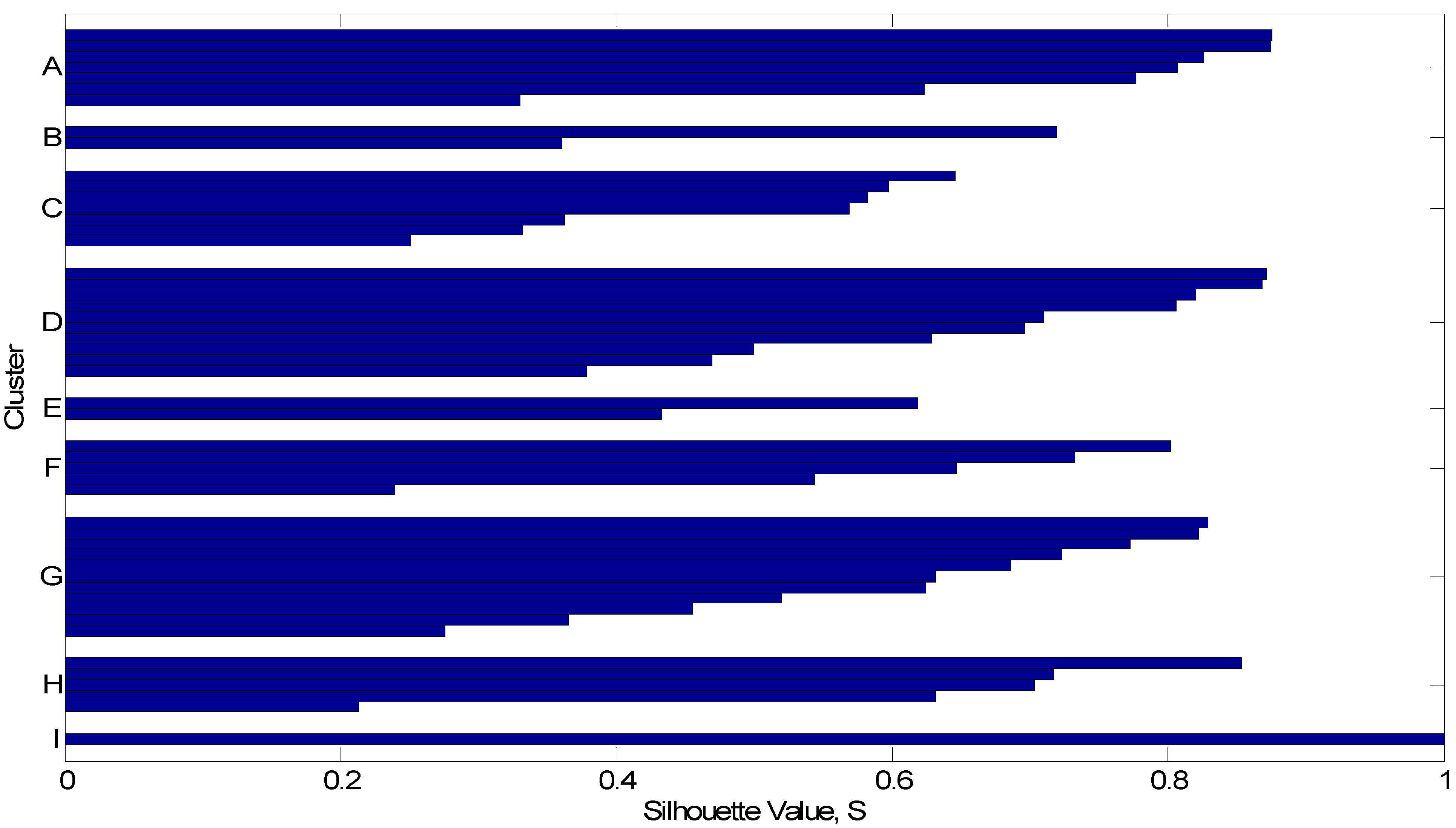
3.1. K-means Analysis Based on G-R Law Parameters

In this subsection the data is analyzed in a per region basis. Events with magnitude M ≥ 4.5 are considered [60]. Above this threshold the cumulative number of earthquakes obeys the G-R law. The corresponding (a, b) parameters, as well as the coefficients of determination of each fit, R, are shown in Table 2.
Table 2. G-R law parameters corresponding to the data of each F-E region. The time period of analysis is 1962–2011. Events with magnitude M ≥ 4.5 are considered.
Region numberabR
18.71.080.99
26.50.880.99
37.00.890.99
47.51.060.99
58.41.100.98
68.41.120.99
78.61.190.99
88.91.080.99
97.41.080.97
108.31.070.92
117.60.970.99
129.41.150.97
139.31.240.97
148.51.020.98
158.51.020.98
168.61.050.96
178.31.160.97
189.51.270.98
199.01.060.99
208.01.050.99
217.60.950.99
228.91.110.98
239.31.180.96
249.21.140.98
257.40.990.99
268.11.070.99
277.30.970.99
287.20.960.99
298.31.120.98
308.41.120.97
318.31.180.98
329.11.210.99
338.81.160.98
347.41.100.96
356.91.240.97
368.11.350.98
378.31.140.99
387.61.150.97
397.61.070.98
407.91.110.98
417.10.940.99
426.80.960.98
438.41.100.96
448.91.320.98
457.10.940.91
468.01.000.99
477.51.050.99
488.71.190.99
496.10.970.94
506.01.090.98
The (a, b) parameters are analyzed using the non-hierarchical clustering technique K-means. We adopt K = 9 clusters as a compromise between a reliable interpretation of the maps and how well-separated the resulting clusters are. The obtained partition is depicted in Figure 1, where the axes values are normalized by the corresponding maximum values. Figure 2 shows the silhouette diagram. The silhouette value, for each object, is a measure of how well each object lies within its cluster [61]. Silhouette values vary in the interval S = –1 to S = +1 and are computed as
S ( n ) = b ( n ) a ( n ) max { b ( n ) , a ( n ) }
where a(n) is the average dissimilarity between object n and all other objects in the cluster to which the object n belongs, ck. On the other hand, b(n) represents the average dissimilarity between object n and the objects in the cluster closest to ck. Silhouette values closer to S = +1 correspond to objects that are very distant from neighboring clusters and, therefore, they are assigned to the right cluster. For S = 0 the objects could be assigned to another cluster. When S = –1 the objects are assigned to the wrong cluster.
From Figure 1, we obtain the K = 9 clusters: 𝒜 = {4, 9, 34, 38, 39, 40, 47}, = {36, 44}, 𝒞 = {10, 14, 15, 16, 20, 26, 46}, 𝒟 = {2, 3, 11, 21, 25, 27, 28, 41, 42, 45}, = {49, 50}, = {1, 8, 19, 22, 24}, 𝒢 = {5, 6, 7, 17, 29, 30, 31, 33, 37, 43, 48}, = {12, 13, 18, 23, 32}, = {35}. Adopting the same colour map used in Figure 1, we depict the F-E regions in the geographical map of Figure 3. It can be noted that the obtained clusters correspond quite well to large contiguous regions.
Figure 1. K-means clustering of all F-E regions and Voronoi cells. Analysis based on the (a, b) parameters of the G-R law. The time period of analysis is 1962–2011. Events with magnitude M ≥ 4.5 are considered.
Entropy 15 03892 g001
Figure 2. Silhouette corresponding to the K-means clustering of all F-E regions. Analysis based on the (a, b) parameters of the G-R law. The time period of analysis is 1962–2011. Events with magnitude M ≥ 4.5 are considered.
Entropy 15 03892 g002
Figure 3. Geographical map of the F-E regions adopting the same colour map used in Figure 1 (green lines correspond to tectonic faults).
Entropy 15 03892 g003

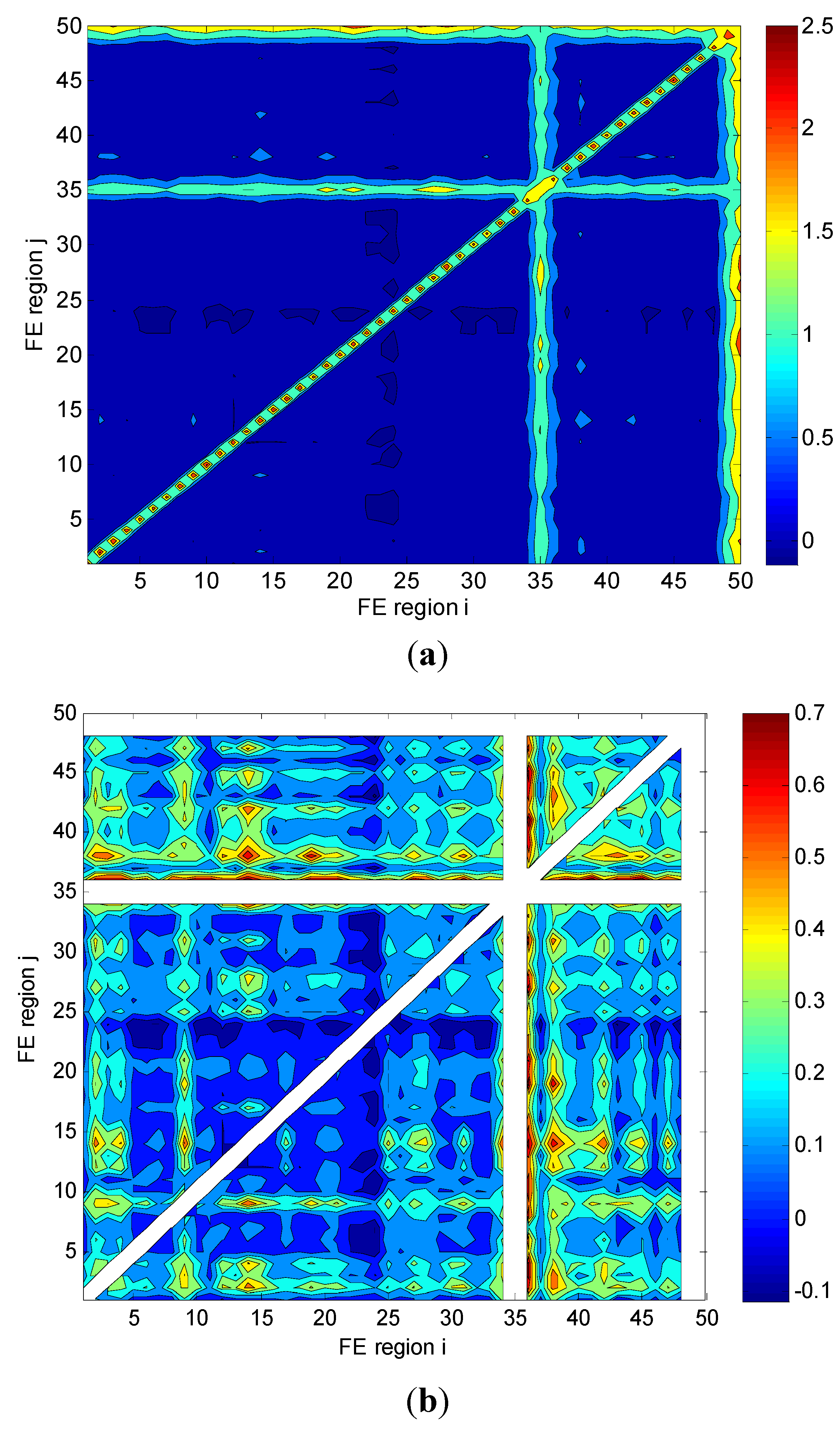
3.2. Analysis by Means of Mutual Information

In this subsection we take the magnitude of the events as random variable and adopt the mutual information as a measurement of similarities between regions i and j (i, j = 1, …, 50). To avoid the systematic bias that occurs when estimating the mutual information from finite data samples we use the expression [62]:
I ( X , Y ) = I h i s t ( X , Y ) + B x + B y B x y 1 2 m ln ( 2 )
I h i s t ( X , Y ) = r = 1 N x s = 1 N y D x y ( r , s ) log 2 [ D x y ( r , s ) D x ( r ) D y ( s ) ]
where mN is the number of data samples, (Nx, Ny) represent number of bins, [Dx(r), Dy(s)] denote the ratios of points belonging to the (rth, sth) bins and Dxy(r, s) is the ratio of points in the intersection of the (rth, sth) bins of the random variables. This means that probability density functions p(x), p(y) and p(x, y) are estimated via a histogram method, where p(x) = Dx(rδx(r)−1, p(y) = Dy(sδy(s)−1, p(x, y) = Dxy(r, sδx(r)−1·δy(s)−1, and [δx(r), δy(s)] represent the size of the (rth, sth) bins. Parameters (Bx, By) represent the number of bins, where [Dx(r) ≠ 0, Dy(s) ≠ 0] and Bxy is the number of bins where Dxy(r, s) ≠ 0. In this study we adopt Nx = Ny = 94.
Based on the mutual information, a 50 × 50 symmetric matrix, IXY, is computed and hierarchical clustering analysis is adopted to reveal the relationships between the F-E regions under analysis.
Figure 4a depicts the mutual information as a contour map. As can be seen, the mutual information between F-E regions #35, #49 and #50 and the rest is remarkable higher, hiding the relationships among most regions. We removed F-E regions #35, #49 and #50 and plotted the corresponding mutual information contour map in Figure 4b.
Figure 4. Mutual information represented as a contour map. (a) all F-E regions are considered; (b) F-E regions #35, #49 and #50 were deleted. The time period of analysis is 1962–2011.
Entropy 15 03892 g004
As the graphs in Figure 4 are difficult to analyze, a hierarchical clustering algorithm is adopted for comparing results (Section 2.4.). We used the phylogenetic analysis open source software PHYLIP [63].
The corresponding circular phylograms are generated by successive (agglomerative) clustering and represented in Figure 5a (for all F-E regions) and 5b (for all F-E regions except #35, #49 and #50). The leaves of the phylograms represent F-E regions. An average-linkage method was used to generate the trees.
Figure 5. Circular phylogram, based on mutual information, used to compare F-E regions. (a) all F-E regions are considered. (b) F-E regions #35, #49 and #50 were deleted. The time period of analysis is 1962–2011.
Entropy 15 03892 g005
Regarding Figure 5a, cluster {35, 49, 50} is clearly different from the rest, as expected. Moreover, clusters {9, 34, 36, 38}, {11, 28, 42}, {26, 39, 47} and {2, 4, 7, 45} can be identified. A larger cluster contains all the rest. Additionally, in Figure 5b, the clusters {3, 27, 29, 31, 40} and {8, 12, 13, 14, 15, 30}, for example, are easily noted, as well as the main larger cluster composed by the remaining F-E regions. Comparing the results coming from the analysis by means of G-R law parameters and mutual information, namely Figure 1 and Figure 5, we can see that the latter is easier to interpret. However, deciding for one or another approach necessitates a more detailed analysis based on specific evidences and practical knowledge in the field. In conclusion, the proposed analysis, based in seismic data catalogues, can help in understanding the overall complex dynamics of earthquakes.

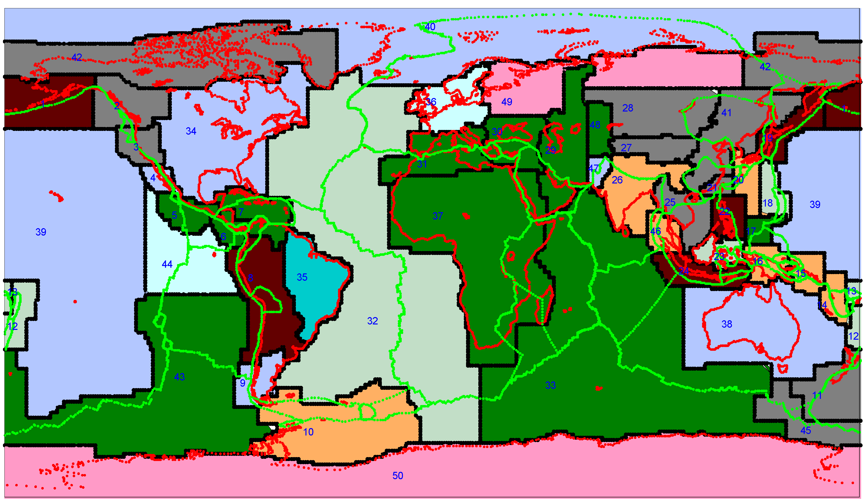
4. Analysis of Rectangular Grid-Based Regions

In this section, instead of F-E regions, an alternative seismic regionalization is considered. The mathematical tools presented in Section 3 are also adopted. We propose dividing Earth into 14 × 14 rectangular cells and, as previously, analyzing data in a per region basis. Events with magnitude M ≥ 4.5 and time period 1962–2011 are considered. The G-R law parameters (a, b) are computed for each region and the results are depicted in Figure 6 and Figure 7, respectively.
Figure 6. Regional variation of G-R parameter a. A 14 × 14 rectangular grid is adopted and events with magnitude M ≥ 4.5 are considered. The time period of analysis is 1962–2011.
Entropy 15 03892 g006
Figure 7. Regional variation of G-R parameter b. A 14 × 14 rectangular grid is adopted and events with magnitude M ≥ 4.5 are considered. The time period of analysis is 1962–2011.
Entropy 15 03892 g007
It can be seen that the activity level parameter, a, assumes larger values in areas of larger seismicity that develop closer to tectonic faults. The scaling exponent, b, reveals identical behavior, being remarkable higher in Scandinavia, Northern Atlantic, Arabic Peninsula, Russian Far East, Brazilian Northeast and Fiji/Tonga/Samoa region. Alternatively, the mutual information is computed and a phylogram is generated to facilitate visualization for the 14 × 14 grid (Figure 8 and Figure 9).
Figure 8. Contour plot representing the mutual information. A 14 × 14 rectangular grid is adopted and events with magnitude M ≥ 4.5 are considered. The time period of analysis is 1962–2011.
Entropy 15 03892 g008
Figure 9. Circular phylogram based on mutual information. A 14 × 14 rectangular grid is adopted and events with magnitude M ≥ 4.5 are considered. The time period of analysis is 1962–2011.
Entropy 15 03892 g009
We observe that the analysis based on the Cartesian grid leads to a more comprehensive visualization of the information than the Flinn-Engdahl regions. Therefore, this approach should be considered as an important alternative to classical definitions of geographical layouts for studying the mutual influence of earthquake and geological data.

5. Conclusions

Based on the magnitudes of the seismic events available in the ISC global catalogue, two schemes were proposed to compare the seismic activity between Earth’s regions. A first method consisted in approximating the data by R-G law and analyzing the parameters that define the distributions shape. The second method used the mutual information as a measure of similarity between regions. In both cases clustering analysis was adopted to visualize the relationships between the data. Different measures lead to distinct results. The mutual information based measure gives results easier to interpret. Both measures can help in understanding the overall complex dynamics of earthquake phenomena.

Conflicts of Interest

The authors declare no conflict of interest.

References

  1. Ghobarah, A.; Saatcioglu, M.; Nistor, I. The impact of the 26 December 2004 earthquake and tsunami on structures and infrastructure. Eng. Struct. 2006, 28, 312–326. [Google Scholar] [CrossRef]
  2. Marano, K.; Wald, D.; Allen, T. Global earthquake casualties due to secondary effects: a quantitative analysis for improving rapid loss analyses. Nat. Hazards 2010, 52, 319–328. [Google Scholar] [CrossRef]
  3. Lee, S.; Davidson, R.; Ohnishi, N.; Scawthorn, C. Fire following earthquake—Reviewing the state-of-the-art modelling. Earthq. Spectra 2008, 24, 933–967. [Google Scholar] [CrossRef]
  4. Bird, J.F.; Bommer, J.J. Earthquake losses due to ground failure. Eng. Geol. 2004, 75, 147–179. [Google Scholar] [CrossRef]
  5. Cavallo, E.; Powell, A.; Becerra, O. Estimating the direct economic damages of the earthquake in Haiti. Econ. J. 2010, 120, 298–312. [Google Scholar] [CrossRef]
  6. Tseng, C.-P.; Chen, C.-W. Natural disaster management mechanisms for probabilistic earthquake loss. Nat. Hazards 2012, 60, 1055–1063. [Google Scholar] [CrossRef]
  7. Wu, J.; Li, N.; Hallegatte, S.; Shi, P.; Hu, A.; Liu, X. Regional indirect economic impact evaluation of the 2008 Wenchuan Earthquake. Environ. Earth Sci. 2012, 65, 161–172. [Google Scholar] [CrossRef]
  8. Keefer, P.; Neumayer, E.; Plümper, T. Earthquake propensity and the politics of mortality prevention. World Dev. 2011, 39, 1530–1541. [Google Scholar] [CrossRef] [Green Version]
  9. Zamani, A.; Agh-Atabai, M. Multifractal analysis of the spatial distribution of earthquake epicenters in the Zagros and Alborz-Kopeh Dagh regions of Iran. Iran J. Sci. Technol. 2011, A1, 39–51. [Google Scholar]
  10. Sornette, D.; Pisarenko, V. Fractal plate tectonics. Geophys. Res. Lett. 2003. [Google Scholar] [CrossRef]
  11. Bhattacharya, P.; Chakrabarti, B.; Kamal. A fractal model of earthquake occurrence: Theory, simulations and comparisons with the aftershock data. J. Phys. Conf. Ser. 2011, 319, 012004. [Google Scholar] [CrossRef]
  12. De Rubeis, V.; Hallgass, R.; Loreto, V.; Paladin, G.; Pietronero, L.; Tosi, P. Self-affine asperity model for earthquakes. Phys. Rev. Lett. 1996, 76, 2599–2602. [Google Scholar] [CrossRef] [PubMed]
  13. Hallgass, R.; Loreto, V.; Mazzella, O.; Paladin, G.; Pietronero, L. Earthquake statistics and fractal faults. Phys. Rev. E 1997, 56, 1346–1356. [Google Scholar] [CrossRef]
  14. Sarlis, N.V.; Christopoulos, S.-R.G. Natural time analysis of the centennial earthquake catalog. Chaos 2012, 22, 023123. [Google Scholar] [CrossRef] [PubMed]
  15. Turcotte, D.L.; Malamud, B.D. International Handbook of Earthquake and Engineering Seismology; Jennings, P., Kanamori, H., Lee, W., Eds.; Academic Press: San Francisco, CA, USA, 2002; p. 209. [Google Scholar]
  16. Kanamori, H.; Brodsky, E. The physics of earthquakes. Rep. Prog. Phys. 2004, 67, 1429–1496. [Google Scholar] [CrossRef]
  17. Stein, S.; Liu, M.; Calais, E.; Li, Q. Mid-continent earthquakes as a complex system. Seismol. Res. Lett. 2009, 80, 551–553. [Google Scholar] [CrossRef]
  18. Lennartz, S.; Livina, V.N.; Bunde, A.; Havlin, S. Long-term memory in earthquakes and the distribution of interoccurrence times. Europhys. Lett. 2008, 81, 69001. [Google Scholar] [CrossRef]
  19. El-Misiery, A.E.M.; Ahmed, E. On a fractional model for earthquakes. Appl. Math. Comput. 2006, 178, 207–211. [Google Scholar] [CrossRef]
  20. Lopes, A.M.; Tenreiro Machado, J.A.; Pinto, C.M.A.; Galhano, A.M.S.F. Fractional dynamics and MDS visualization of earthquake phenomena. Comput. Math. Appl. 2013, 66, 647–658. [Google Scholar] [CrossRef]
  21. Sornette, A.; Sornette, D. Self-organized criticality and earthquakes. Europhys. Lett. 1989, 9, 197–202. [Google Scholar] [CrossRef]
  22. Shahin, A.M.; Ahmed, E.; Elgazzar, A.S.; Omar, Y.A. On fractals and fractional calculus motivated by complex systems. 2009. [Google Scholar]
  23. Rocco, A.; West, B.J. Fractional calculus and the evolution of fractal phenomena. Physica A 1999, 265, 535–546. [Google Scholar] [CrossRef]
  24. Samko, S.; Kilbas, A.; Marichev, O. Fractional Integrals and Derivatives: Theory and Applications; Gordon and Breach Science Publishers: London, UK, 1993. [Google Scholar]
  25. Podlubny, I. Fractional Differential Equations; Academic Press: San Diego, CA, USA, 1999. [Google Scholar]
  26. Kilbas, A.; Srivastava, H.M.; Trujillo, J. Theory and Applications of Fractional Differential Equations; Elsevier: Amsterdam, The Netherlands, 2006. [Google Scholar]
  27. Baleanu, D.; Diethelm, K.; Scalas, E.; Trujillo, J. Fractional Calculus: Models and Numerical Methods; Series on Complexity, Nonlinearity and Chaos; World Scientific Publishing: Singapore, Singapore, 2012. [Google Scholar]
  28. International Seismological Centre (2010) On-line Bulletin, Internatl. Seis. Cent., Thatcham, UK. Available online: http://www.isc.ac.uk (accessed on 12 June 2013).
  29. Gutenberg, B.; Richter, C.F. Frequency of earthquakes in California. Bull. Seismol. Soc. Am. 1944, 34, 185–188. [Google Scholar]
  30. Christensen, K.; Olami, Z. Variation of the Gutenberg-Richter b values and nontrivial temporal correlations in a spring-block model for earthquakes. J. Geophys. Res. 1992, 97, 8729–8735. [Google Scholar] [CrossRef]
  31. Ogata, Y.; Katsura, K. Analysis of temporal and spatial heterogeneity of magnitude frequency distribution inferred from earthquake catalogues. Geophys. J. Int. 1993, 113, 727–738. [Google Scholar] [CrossRef]
  32. Shannon, C.E. A mathematical theory of communication. Bell Syst. Tech. J. 1948, 27, 379–423, 623–656. [Google Scholar] [CrossRef]
  33. Posadas, A.; Hirata, T.; Vidal, F.; Correig, A. Spatio-temporal seismicity patterns using mutual information application to southern Iberian peninsula (Spain) earthquakes. Phys. Earth Planet. Inter. 2000, 122, 269–276. [Google Scholar] [CrossRef]
  34. Telesca, L. Tsallis-based nonextensive analysis of the southern California seismicity. Entropy 2011, 13, 1267–1280. [Google Scholar] [CrossRef]
  35. Mohajeri, N.; Gudmundsson, A. Entropies and scaling exponents of street and fracture networks. Entropy 2012, 14, 800–833. [Google Scholar] [CrossRef]
  36. Matsuda, H. Physical nature of higher-order mutual information: Intrinsic correlations and frustration. Phys. Rev. E 2000, 62, 3096–3102. [Google Scholar] [CrossRef]
  37. Fraser, A.M.; Swinney, H.L. Independent coordinates for strange attractors from mutual information. Phys. Rev. A 1986, 33, 1134–1140. [Google Scholar] [CrossRef] [PubMed]
  38. Vastano, J.A.; Swinney, H.L. Information transport in spatiotemporal systems. Phys. Rev. Lett. 1988, 60, 1773–1776. [Google Scholar] [CrossRef] [PubMed]
  39. Fraser, A.M. Reconstructing attractors from scalar time series: A Comparison of singular system and redundancy criteria. Phys. D 1989, 34, 391–404. [Google Scholar] [CrossRef]
  40. Herzel, H.; Schmitt, A.O.; Ebeling, W. Finite sample effects in sequence analysis. Chaos Soliton Fractals 1994, 4, 97–113. [Google Scholar] [CrossRef]
  41. Tenreiro Machado, J.A.; Costa, A.C.; Quelhas, M.D. Entropy analysis of DNA code dynamics in human chromosomes. Comput. Math. Appl. 2011, 62, 1612–1617. [Google Scholar] [CrossRef]
  42. Tenreiro Machado, J.A.; Costa, A.C.; Quelhas, M.D. Shannon, Rényie and Tsallis entropy analysis of DNA using phase plane. Nonlinear Anal. Real World Appl. 2011, 12, 3135–3144. [Google Scholar] [CrossRef]
  43. Matsuda, H.; Kudo, K.; Nakamura, R.; Yamakawa, O.; Murata, T. Mutual information of Ising systems. Int. J. Theor. Phys. 1996, 35, 839–845. [Google Scholar] [CrossRef]
  44. Mori, T.; Kudo, K.; Tamagawa, Y.; Nakamura, R.; Yamakawa, O.; Suzuki, H.; Uesugi, T. Edge of chaos in rule-changing cellular automata. Phys. D 1998, 116, 275–282. [Google Scholar] [CrossRef]
  45. Feldman, D.P.; Crutchfield, J.P. Measures of statistical complexity: Why? Phys. Lett. A 1998, 238, 244–252. [Google Scholar] [CrossRef]
  46. Wicks, R.T.; Chapman, S.C.; Dendy, R.O. Mutual information as a tool for identifying phase transitions in dynamical complex systems with limited data. Phys. Rev. E 2007, 75, 051125. [Google Scholar] [CrossRef]
  47. Kwapieńa, J.; Drożdż, S. Physical approach to complex systems. Phys. Rep. 2012, 515, 115–226. [Google Scholar] [CrossRef]
  48. Arabie, P.; Hubert, L. Cluster analysis in marketing research. In Advanced Methods in Marketing Research; Bagozzi, R.P., Ed.; Blackwell: Oxford, UK, 1994; p. 160. [Google Scholar]
  49. Bishop, C.M. Pattern Recognition and Machine Learning; Springer-Verlag: New York, NY, USA, 2006. [Google Scholar]
  50. Park, U.; Jain, A.K. Face matching and retrieval using soft biometrics. IEEE Trans. Inf. Forensics Secur. 2010, 5, 406–415. [Google Scholar] [CrossRef]
  51. Cover, T.M.; Thomas, J.A. Elements of Information Theory; John Wiley & Sons: New York, NY, USA, 1991. [Google Scholar]
  52. Jain, A.K. Data clustering: 50 years beyond K-means. Pattern Recognit. Lett. 2010, 31, 651–666. [Google Scholar] [CrossRef]
  53. Kanungo, T.; Mount, D.M.; Netanyahu, N.S.; Piatko, C.D.; Silverman, R.; Wu, A.Y. An efficient K-means clustering algorithm: Analysis and implementation. IEEE Trans. Pattern Anal. 2002, 24, 881–892. [Google Scholar] [CrossRef]
  54. Jain, A.K.; Dubes, R. Algorithms for Clustering Data; Prentice-Hall: Englewood Cliffs, NJ, USA, 1988. [Google Scholar]
  55. Johnson, S.C. Hierarchical clustering schemes. Psychometrika 1966, 32, 241–254. [Google Scholar] [CrossRef]
  56. Gower, J.C.; Ross, G.J.S. Minimum spanning trees and single linkage cluster analysis. Appl. Stat. 1969, 18, 54–64. [Google Scholar] [CrossRef]
  57. Ward, J.H., Jr. Hierarchical grouping to optimize an objective function. J. Am. Stat. Assoc. 1963, 58, 236–244. [Google Scholar] [CrossRef]
  58. Flinn, E.A.; Engdahl, E.R.; Hill, A.R. Seismic and geographical regionalization. Bull. Seismol. Soc. Am. 1974, 64, 771–993. [Google Scholar]
  59. Flinn, E.A.; Engdahl, E.R. A proposed basis for geographical and seismic regionalization. Rev. Geophys. 1965, 3, 123–149. [Google Scholar] [CrossRef]
  60. Zhao, X.; Omi, T.; Matsuno, N.; Shinomoto, S. A non-universal aspect in the temporal occurrence of earthquakes. New J. Phys. 2010, 12, 063010. [Google Scholar] [CrossRef]
  61. Rousseeuw, P.J. Silhouettes: A graphical aid to the interpretation and validation of cluster analysis. J. Comput. Appl. Math. 1987, 20, 53–65. [Google Scholar] [CrossRef]
  62. Omi, T.; Kanter, I.; Shinomoto, S. Optimal observation time window for forecasting the next earthquake. Phys. Rev. E 2011, 83, 026101. [Google Scholar] [CrossRef] [Green Version]
  63. Felsenstein, J. PHYLIP, version 3.6; free phylogeny inference package; Distributed by the author; Department of Genome Sciences, University of Washington: Seattle, Washington, DC, USA, 2005. [Google Scholar]

