Analysis of Time Reversible Born-Oppenheimer Molecular Dynamics ^†

Abstract

We analyze the time reversible Born-Oppenheimer molecular dynamics (TRBOMD) scheme, which preserves the time reversibility of the Born-Oppenheimer molecular dynamics even with non-convergent self-consistent field iteration. In the linear response regime, we derive the stability condition, as well as the accuracy of TRBOMD for computing physical properties, such as the phonon frequency obtained from the molecular dynamics simulation. We connect and compare TRBOMD with Car-Parrinello molecular dynamics in terms of accuracy and stability. We further discuss the accuracy of TRBOMD beyond the linear response regime for non-equilibrium dynamics of nuclei. Our results are demonstrated through numerical experiments using a simplified one-dimensional model for Kohn-Sham density functional theory.

1. Introduction

Ab initio molecular dynamics (AIMD) [1–6] has been greatly developed in the past few decades, so that nowadays, it is able to quantitatively predict the equilibrium and non-equilibrium properties for a vast range of systems. AIMD has become widely used in chemistry, biology, materials science, etc. A coherent and comprehensive presentation of AIMD with both the basic theory and advanced methods can be found in [7]. Most AIMD methods treat the nuclei as classical particles following Newtonian dynamics (known as the time-dependent Born-Oppenheimer approximation), and the interactive force among nuclei is provided directly from electronic structure theory, such as the Kohn-Sham density functional theory [8,9] (KSDFT), without the need of using empirical atomic potentials. KSDFT consists of a set of nonlinear equations that are solved at each molecular dynamics time step self-consistently via the self-consistent field (SCF) iteration. In Born-Oppenheimer molecular dynamics (BOMD), KSDFT is solved until full self-consistency for each atomic configuration per time step. Since many iterations are usually needed to reach full self-consistency and each iteration takes a considerable amount of time, until recently, this procedure was still found to be prohibitively expensive for producing meaningful dynamical information. On the other hand, if the self-consistent iterations are truncated before convergence is reached, it is often the case that the energy of the system is no longer conservative, even for an NVE system. The error in SCF iteration acts as a sink or source, gradually draining or adding energy to the atomic system within a short period of molecular dynamics simulation [10]. This is one of the main challenges for accelerating Born-Oppenheimer molecular dynamics.

AIMD was made practical by the ground-breaking work of Car-Parrinello molecular dynamics (CPMD) [11]. CPMD introduces an extended Lagrangian, including the degrees of freedom of both nuclei and electrons without the necessity of a convergent SCF iteration. The dynamics of electronic orbitals can be loosely viewed as a special way for performing the SCF iteration at each molecular dynamics (MD) step. Thanks to the Hamiltonian structure, numerical simulation for CPMD is stable, and the energy is conservative over a much longer time period compared to that for BOMD with non-convergent SCF iteration. When the system has a spectral gap, the accuracy of CPMD is controlled by a single parameter, the fictitious electron mass, μ. The result of CPMD approaches that of BOMD as μ goes to zero [12,13]. However, it has also been shown that CPMD does not work as well for systems with a vanishing gap, for example, for metallic systems [12].

To reduce the cost of BOMD, in particular, the number of SCF iterations needed per MD time step, a new type of AIMD method, the time reversible Born-Oppenheimer molecular dynamics (TRBOMD) method has been recently proposed by Niklasson, Tymczak and Challacombe in [14]. The method has been further developed in [15–18]. The idea of TRBOMD can be summarized as follows: TRBOMD assumes that the SCF iteration is a deterministic procedure, with the outcome determined only by the initial guess of the variable to be determined self-consistently. For instance, this variable can be the electron density, and the SCF iteration procedure can be simple mixing with a fixed number of iteration steps without reaching full self-consistency. Then, a fictitious dynamics governed by a second order ordinary differential equation (ODE) is introduced on this initial guess variable. The resulting coupled dynamics is then time-reversible and supposed to be more stable, since it has been found that time-reversible numerical schemes are more stable for long time simulation [19,20]. Besides TRBOMD, alternative ideas based on time-reversible predictor-corrector methods [21] and Langevin dynamics [22,23] can also relax the requirement on the accuracy of the force for AIMD simulation. For these methods, we refer the readers to a recent review paper [24] for more information.

Although TRBOMD has been found to be effective and significantly reduces the number of SCF iterations needed in practice, to the extent of our knowledge, there has been so far no detailed analysis of TRBOMD, other than the numerical stability condition of the Verlet or generalized Verlet scheme for time discretization [17]. Accuracy, stability, as well as the applicability range of TRBOMD remain unclear. In particular, it is not known how the choice of SCF iteration scheme affects TRBOMD. These are crucial issues for guiding the practical use of TRBOMD. The full TRBOMD method for general systems is highly nonlinear and is difficult to analyze. In this work, we first focus on the linear response regime, i.e., we assume that each atom oscillates around their equilibrium position and the electron density stays around the “true” electron density. Under such assumptions, we analyze the accuracy and stability of TRBOMD. We then extend the results to the regime where the atom position is not near equilibrium using the averaging principle.

The rest of the paper is organized as follows. We illustrate the idea of TRBOMD and its analysis in the linear response regime using a simple model in Section 2 and introduce TRBOMD for AIMD in Section 3. We analyze TRBOMD in the linear response regime and compare TRBOMD with CPMD in Section 4. The numerical results for TRBOMD in the linear response regime are given in Section 5. We present the analysis of TRBOMD beyond the linear response regime, such as the non-equilibrium dynamics in Section 6, and conclude with a few remarks in Section 7.

2. An Illustrative Model

To start, let us illustrate the main idea for a simple model problem, which provides the essence of TRBOMD in a much simplified setting. Consider the following nonlinear ODE:

$$\ddot{x}(t)=f(x(t))$$

(1)

where we assume that the right-hand side f(x) is difficult to compute, and it can be approximated by an iterative procedure. Starting from an initial guess, s ≈ f(x), the final approximation via the iterative procedure is denoted by g(x, s). We assume the approximation, g(x, s), is consistent, i.e:

$$g(x,f(x))=f(x)$$

(2)

To numerically solve the ODE Equation (1), we discretize it by some numerical scheme; then, it remains to decide the initial guess, s, at each time step. A natural choice of s would be g(x, s) from the previous step, as x does not change much in successive steps. For instance, if the Verlet algorithm is used and t_k = kΔt with Δt being the time step, the discretized ODE becomes:

$$\begin{array}{l}{x}_{k+1}=2x_k-x_{k-1}+{\left(\Delta t\right)}^{2}g\left(x_k,s_k\right)\\ s_{k+1}=g\left(x_k,s_k\right)\end{array}$$

(3)

We immediately observe that the discretization scheme Equation (3) breaks the time reversibility of the original ODE Equation (1). In other words, for the original ODE Equation (1), we propagate the system forward in time from (x(t₀), ẋ(t₀)) to (x(t₁), ẋ(t₁)). Then, if we use (x(t₁), ẋ(t₁)) as the initial data at t = t₁ and propagate the system backward in time to time t = t₀, we will be at the state, (x(t₀), ẋ(t₀)). The loss of the time reversible structure can introduce large error in long time numerical simulation [20]. This is the main reason why BOMD with non-convergent SCF iteration fails for long time simulations [14]. To overcome this obstacle, the idea of TRBOMD is to introduce a fictitious dynamics for the initial guess, s. Namely, we consider the time reversible coupled system:

$$\begin{array}{l}\ddot{x}(t)=g\left(x(t),s(t)\right)\\ \ddot{s}(t)={\omega }^2(g\left(x(t),s(t))-s(t)\right)\end{array}$$

(4)

where ω is an artificial frequency. We analyze, now, the accuracy and stability of Equation (4) in the linear response regime by assuming that the trajectory, x(t), oscillates around an equilibrium position, x^*. We denote by x̃(t) = x(t) − x^*the deviation from the equilibrium position and s̃(t) = s(t) − f(x(t)), the deviation of the initial guess from the exact force term. Consequently, the equation of motion (4) can be rewritten as (for simplicity we suppress the t-dependence in the notation for the rest of the section):

$$\begin{array}{l}\ddot{\tilde{x}}=g(x,s)\\ \ddot{\tilde{s}}={\omega }^2(g(x,s)-s)-f^{″}(x){\left(\dot{x}\right)}^2-f^{\prime }(x)\ddot{x}\end{array}$$

(5)

where the term, −f″(x)(ẋ)²− f′(x)ẍ, comes from the term, f(x) in s̃, by the chain rule.

In the linear response regime, we assume the linear approximation of force for x around x^*:

$$f(x)\approx -{\Omega }^2(x-x^{*})=-{\Omega }^2\tilde{x}$$

(6)

where Ω is the oscillation frequency of x in the linear response regime. We also linearize g with respect to s̃ and x̃ and dropping all higher order terms as:

$$\begin{array}{ll}g(x,s)\hfill & =g(x,f(x)+\tilde{s})\hfill \\ \hfill & \approx g(x,f(x))+g_s(x,f(x))\tilde{s}\hfill \\ \hfill & \approx -{\Omega }^2\tilde{x}+g_s(x^{*},f(x^{*}))\tilde{s}\hfill \end{array}$$

(7)

where g_s denotes the partial derivative of g with respect to s, and the consistency condition (2) is applied. We then have:

$$\begin{array}{ll}g(x,s)-s\hfill & =\left(g(x,f(x)+\tilde{s})-f(x)\right)-(s-f(x))\hfill \\ \hfill & \approx (g_s(x,f(x))-1)\tilde{s}\hfill \\ \hfill & \approx (g_s(x^{*},f(x^{*}))-1)\tilde{s}\hfill \end{array}$$

(8)

In accord with notations used in later discussions, let us denote:

$$ℒ=g_s(x^{*},f(x^{*})),\hspace{0.17em}\hspace{0.17em}\hspace{0.17em}\hspace{0.17em}\hspace{0.17em}𝒦=1-g_s(x^{*},f(x^{*}))$$

(9)

with which the linearized system of Equation (5) becomes:

$$\frac{{\text{d}}^2}{\text{d}{t}^2}\left(\begin{array}{l}\tilde{x}\hfill \\ \tilde{s}\hfill \end{array}\right)=\left(\begin{array}{cc}-{\Omega }^2& ℒ\\ f^{\prime }(x^{*}){\Omega }^2& -f^{\prime }(x^{*})ℒ-{\omega }^2𝒦\end{array}\right)\left(\begin{array}{l}\tilde{x}\hfill \\ \tilde{s}\hfill \end{array}\right):=A\left(\begin{array}{l}\tilde{x}\hfill \\ \tilde{s}\hfill \end{array}\right)$$

(10)

Note that when the force is computed accurately, i.e.,

$$g(x,s)=f(x),\hspace{0.17em}\hspace{0.17em}\hspace{0.17em}\hspace{0.17em}\forall s$$

(11)

we have:

$$ℒ=0,\hspace{0.17em}\hspace{0.17em}\hspace{0.17em}\hspace{0.17em}\hspace{0.17em}𝒦=1$$

(12)

meaning that the motion of x̃ is decoupled from that of s̃, and x̃ follows the exact harmonic motion in the linear response regime with the accurate frequency, Ω. When the force is computed inaccurately, x̃ is coupled with s̃ in Equation (10). Actually, we can solve (10) analytically, and the eigenvalues of A are:

$$\left(\begin{array}{c}{\lambda }_{\tilde{\Omega }}\\ {\lambda }_{\tilde{\omega }}\end{array}\right)=\left(\begin{array}{c}\frac{1}{2}\left(\sqrt{{\left(ℒf^{\prime }(x*)+𝒦{\omega }^2+{\Omega }^2\right)}^2-4𝒦{\omega }^2{\Omega }^2}-ℒf^{\prime }(x^{*})-𝒦{\omega }^2-{\Omega }^2\right)\\ \frac{1}{2}\left(-\sqrt{{\left(ℒf^{\prime }(x*)+𝒦{\omega }^2+{\Omega }^2\right)}^2-4𝒦{\omega }^2{\Omega }^2}-ℒf^{\prime }(x^{*})-𝒦{\omega }^2-{\Omega }^2\right)\end{array}\right)$$

(13)

Then, the frequencies of the normal modes of the ODE are $\tilde{\Omega }=\sqrt{-{\lambda }_{\tilde{\Omega }}}$ and $\tilde{\omega }=\sqrt{-{\lambda }_{\tilde{\omega }}}$ respectively. Assume ω² ≫ Ω² and expand the solution to the order of $𝒪$(1/ω²); we have:

$$\tilde{\Omega }=\Omega \left(1-\frac{f^{\prime }(x^{*})}{2{\omega }^2}ℒ{𝒦}^{-1}\right)+𝒪(1/{\omega }^4)$$

(14)

Similarly, the frequency for the other normal mode, which is dominated by the motion of s̃, is:

$$\tilde{\omega }=\sqrt{𝒦}\omega \left(1+\frac{f^{\prime }(x^{*})}{2{\omega }^2}ℒ{𝒦}^{-1}\right)+𝒪(1/{\omega }^3)$$

(15)

It is found that one of the normal modes of Equation (10) has frequency Ω̃ ≈ Ω. We can therefore measure the accuracy of Equation (4) using the relative error between Ω̃ and Ω. Furthermore, if the dynamics (4) is stable in the linear response regime, it is necessary to have $𝒦$ > 0.

From Equation (14), we conclude that if the time reversible numerical scheme (4) is used for simulating the ODE Equation (1) and if we neglect the error due to the Verlet scheme, the error introduced in computing the frequency, Ω, is proportional to ω⁻². This seems to indicate that very large ω (i.e., very small time step Δt) might be needed to obtain accurate results. Fortunately, the ω⁻² term in Equation (14) has the prefactor, f′(x^*)$ℒ$$𝒦$⁻¹. Equation (6) shows that f′(x^*) ≈ −Ω², which is small compared to ω². If g_s(x^*, f(x^*)) is small, then $𝒦$ ≈ 1, and the accuracy of Ω̃ is determined by $ℒ$ or g_s(x^*, f(x^*)), which indicates the sensitivity of the computed force with respect to the initial guess, or the accuracy of the iterative procedure for computing the force. If a “good” iterative procedure is used, g_s(x^*, f(x^*)) will be small. Therefore, the presence of the term, $ℒ$, allows one to obtain relatively accurate approximation to the frequency, Ω, without using a large ω. The same behavior can be observed when using TRBOMD to approximate BOMD (vide post).

Finally, we remark that even though Equation (1) is a much simplified system, it will be seen below that for BOMD with M atoms and N interacting electrons, the analysis in the linear response regime follows the same line, and the result for the frequency is similar to Equation (14).

3. Time Reversible Born-Oppenheimer Molecular Dynamics

Consider a system with M atoms and N electrons. The position of the atoms at time t is denoted by R(t) = (R₁(t), …, R_M(t))^T. In BOMD, the motion of atoms follows Newton’s law:

$$m{\ddot{R}}_I(t)=f_I(\mathbf{R}(t))=-\frac{\partial E(\mathbf{R}(t))}{\partial R_I}$$

(16)

where E(R(t)) is the total energy of the system at the atomic configuration, R(t). In KSDFT, the total energy is expressed as a functional of a set of Kohn-Sham orbitals, ${\left\{{\psi }_i(x)\right\}}_{i=1}^N$. To illustrate the idea with minimal technicality, let us consider for the moment a system of N electrons at zero temperature. The energy functional in KSDFT takes the form:

$$\begin{array}{l}E\left({\left\{{\psi }_i(x)\right\}}_{i=1}^N;\mathbf{R}\right)=\frac{1}{2}\sum _{i=1}^N\int {\left|\nabla {\psi }_i(x)\right|}^2\hspace{0.17em}\text{d}x+\int \rho (x)V_{\text{ion}}(x;\mathbf{R})\hspace{0.17em}\text{d}x+E_{\text{hxc}}\left[\rho \right]\\ \hspace{0.17em}\hspace{0.17em}\hspace{0.17em}\hspace{0.17em}\hspace{0.17em}\hspace{0.17em}\hspace{0.17em}\hspace{0.17em}\hspace{0.17em}\hspace{0.17em}\hspace{0.17em}\hspace{0.17em}\hspace{0.17em}\hspace{0.17em}\hspace{0.17em}\hspace{0.17em}\hspace{0.17em}\hspace{0.17em}\hspace{0.17em}\hspace{0.17em}\hspace{0.17em}\hspace{0.17em}\hspace{0.17em}\hspace{0.17em}\hspace{0.17em}\hspace{0.17em}\hspace{0.17em}\hspace{0.17em}\hspace{0.17em}\rho (x)=\sum _{i=1}^N{\left|{\psi }_i(x)\right|}^2\end{array}$$

(17)

The first term in the energy functional is the kinetic energy of the electrons. The second term contains the electron-ion interaction energy. The ion-ion interaction energy usually takes the form ${\sum }_{I<J}\frac{Z_I{Z}_J}{\left|R_I-R_J\right|}$, where Z_I is the charge for the nucleus, I. The ion-ion interaction energy does not depend on the electron density, ρ. To simplify the notation, we include the ion-ion interaction energy in the V_ion term as a constant shift that is independent of the x variable. The third term does not explicitly depend on the atomic configuration, R, and is a nonlinear functional of the electron density, ρ. It represents the Hartree part of electron-electron interaction energy (h) and the exchange-correlation energy (xc) characterizing many body effects. The energy, E(R), as a function of atomic positions is given by the following minimization problem:

$$\begin{array}{l}E(\mathbf{R})=\underset{{\left\{{\psi }_i(x)\right\}}_{i=1}^N}{\text{min}}\hspace{0.17em}E({\left\{{\psi }_i(x)\right\}}_{i=1}^N;\mathbf{R})\\ \text{s}.\text{t}.\hspace{0.17em}\hspace{0.17em}\hspace{0.17em}\hspace{0.17em}\hspace{0.17em}\hspace{0.17em}\hspace{0.17em}\hspace{0.17em}\hspace{0.17em}\int {\psi }_i^{†}(x){\psi }_j(x)\hspace{0.17em}\text{d}x={\delta }_{ij,}\hspace{0.17em}\hspace{0.17em}\hspace{0.17em}\hspace{0.17em}\hspace{0.17em}\hspace{0.17em}\hspace{0.17em}i,j=1,\dots ,N\end{array}$$

(18)

We denote by ${\left\{{\psi }_i(x;\mathbf{R})\right\}}_{i=1}^N$ the (local) minimizer and ${\rho }^{*}(x;\mathbf{R})={{\sum }_{i=1}^N\left|{\psi }_i(x;\mathbf{R})\right|}^2$, the converged electron density corresponding to the minimizer (here, we assume that the minimizing electron density is unique). Then, the force acting on the atom I is:

$$f_I(\mathbf{R};{\rho }^{*}(x;\mathbf{R}))=-\frac{\partial E(\mathbf{R})}{\partial R_I}=-\int {\rho }^{*}(x;\mathbf{R})\frac{\partial V_{\text{ion}}(x;\mathbf{R})}{\partial R_I}\text{d}x$$

(19)

In the physics literature, the force formula in Equation (19) is referred to as the Hellmann-Feynman force. The validity of the Hellmann-Feynman formula relies on the electron density, ρ^*(x; R), corresponding to the minimizers of the Kohn-Sham energy functional. Since E_hxc[ρ] is a nonlinear functional of ρ, the electron density, ρ, is usually determined through the self-consistent field (SCF) iteration as follows.

Starting from an inaccurate input electron density, ρⁱⁿ, one first computes the output electron density by solving the lowest N eigenfunctions of the problem:

$$\left(-\frac{1}{2}{\Delta }_x+𝒱(x;\mathbf{R},{\rho }^{\text{in}})\right){\psi }_i={\varepsilon }_i{\psi }_i$$

(20)

with:

$$𝒱(x;\mathbf{R},\rho )=V_{\text{ion}}(x;\mathbf{R})+\frac{\delta E_{\text{hxc}}\left[\rho \right]}{\delta \rho }(x)$$

(21)

and the output electron density, ρ^out, is defined by:

$${\rho }^{\text{out}}(x):=F\left[{\rho }^{\text{in}}\right](x)=\sum _{i=1}^N{\left|{\psi }_i(x)\right|}^2$$

(22)

Here, the operator, F, is called the Kohn-Sham map. ρ^out can be used directly as the input electron density, ρⁱⁿ, in the next iteration. This is called the fixed point iteration. Unfortunately, in most electronic structure calculations, the fixed point iteration does not converge, even when ρⁱⁿ is very close to the true electron density, ρ^*. The fixed point iteration can be improved by the simple mixing method, which takes the linear combination of the electron density:

$$\alpha {\rho }^{\text{out}}+(1-\alpha ){\rho }^{\text{in}}$$

(23)

as the input density for the next iteration with 0 < α ≤ 1. Simple mixing can greatly improve the convergence properties of the SCF iteration over the fixed point iteration, but the convergence rate can still be slow in practice. There are more complicated SCF iteration schemes, such as the Anderson mixing scheme [25], the Pulay mixing scheme [26] and the Broyden mixing scheme [27]. Furthermore, preconditioners can be applied to the SCF iteration to enhance convergence properties, such as the Kerker preconditioner [28]. More detailed discussion on the convergence properties of these SCF schemes can be found in [29]. In the following discussions, we denote by ρ_SCF(x; R, ρ) the final electron density after the SCF iteration starting from an initial guess, ρ. We assume that ρ_SCF satisfies the consistency condition:

$${\rho }_{\text{SCF}}(x;\mathbf{R},{\rho }^{*}(\cdot ;\mathbf{R}))={\rho }^{*}(x;\mathbf{R})$$

(24)

If a non-convergent SCF iteration procedure is used, ρ_SCF(x; R, ρ) might deviate from ρ^*(x; R). Such deviation introduces error in the force, and the error can accumulate in the long time molecular dynamics simulation and lead to inaccurate results in computing the statistical and dynamical properties of the systems.

The map, ρ_SCF, is usually highly nonlinear, which makes it difficult to correct the error in the force. The TRBOMD scheme avoids the direct correction for the inaccurate ρ_SCF, but allows the initial guess to dynamically evolve together with the motion of the atoms. We denote by ρ(x, t) the initial guess for the SCF iteration at time t. When ρ(·, t) is used as an argument, we also write ρ_SCF(x; R(t), ρ(t)) ≔ ρ_SCF(x; R(t), ρ(·, t)). The Hellmann-Feynman formula (19) is used to compute the force at the electron density, ρ_SCF(x; R(t), ρ(t)), even though ρ^*(x; R(t)) is not available. Thus, the equation of motion in TRBOMD reads:

$$\begin{array}{l}m{\ddot{R}}_I(t)=f_I(\mathbf{R}(t);{\rho }_{\text{SCF}}(x;\mathbf{R}(t),\rho (t)))=-\int {\rho }_{\text{SCF}}(x;\mathbf{R}(t),\rho (t))\frac{\partial V_{\text{ion}}(x;\mathbf{R}(t))}{\partial R_I}\text{d}x\\ \hspace{0.17em}\hspace{0.17em}\hspace{0.17em}\hspace{0.17em}\ddot{\rho }(x,t)={\omega }^2({\rho }_{\text{SCF}}(x;\mathbf{R}(t),\rho (t))-\rho (x,t))\end{array}$$

(25)

It is clear that TRBOMD is time reversible. The discretized TRBOMD is still time reversible if the numerical scheme is time reversible. For instance, if the Verlet scheme is used, the discretized equation of motion becomes:

$$\begin{array}{l}{R}_I\left(t_{k+1}\right)=2R_I\left(t_k\right)-R_I\left(t_{k-1}\right)-\frac{\Delta t^2}{m}{f}_I(\mathbf{R}\left(t_k\right);{\rho }_{\text{SCF}}\left(x;\mathbf{R}\left(t_k\right),\rho \left(t_k\right)\right)\\ \rho \left(x,t_{k+1}\right)=2\rho \left(x,t_k\right)-\rho \left(x,t_{k-1}\right)+\Delta t^2{\omega }^2\left({\rho }_{\text{SCF}}\left(x;\mathbf{R}\left(t_k\right),\rho \left(t_k\right)\right)-\rho \left(x,t_k\right)\right)\end{array}$$

(26)

which is evidently time reversible. The artificial frequency, ω, controls the frequency of the fictitious dynamics of ρ(x, t) and is generally chosen to be larger than the frequency of the motion of the atoms. The numerical stability of the Verlet algorithm requires that the dimensionless quantity, κ≔ (ωΔt)², be small [30]. When κ is fixed, ω controls the stiffness or, equivalently, the time step $\Delta t=\frac{\sqrt{\kappa }}{\omega }$ for the equation of motion (26).

Let us mention that TRBOMD is closely related to CPMD. In CPMD, the equation of motion is given by:

$$\begin{array}{l}m{\ddot{R}}_I\left(t\right)=f_I\left(\mathit{R}\left(t\right),\rho \left(t\right)\right)=-\int \rho \left(t\right)\frac{\partial V_{\text{ion}}\left(x;\mathit{R}\left(t\right)\right)}{\partial R_I}\text{d}x\\ \hspace{0.17em}\hspace{0.17em}\mu {\ddot{\psi }}_i\left(t\right)=-\frac{\delta E\left(\mathit{R}\left(t\right),\left\{{\psi }_i\left(t\right)\right\}\right)}{\delta {\psi }_i^{†}}+\sum _j{\psi }_j\left(t\right){\Lambda }_{ji}\left(t\right)\end{array}$$

(27)

where μ is the fictitious electron mass for the fake electron dynamics in CPMD and Λ’s are the Lagrange multipliers determined so that {ψ_i(t)} is an orthonormal set of functions for any time. The CPMD scheme (27) can be viewed as the equation of motion with an extended Lagrangian:

$${ℒ}_{\text{CP}}\left(\mathit{R},\dot{\mathit{R}},\left\{{\psi }_i\right\},\left\{{\dot{\psi }}_i\right\}\right)=\sum _I\frac{m}{2}{\left|{\dot{R}}_I\right|}^2+\sum _i\frac{\mu }{2}\int {\left|{\dot{\psi }}_i\right|}^2-E\left(\mathit{R},\left\{{\psi }_i\right\}\right)$$

(28)

which contains both ionic and electronic degrees of freedom. Therefore, CPMD is a Hamiltonian dynamics and, thus, time reversible.

Note that the frequency of the evolution equation for {ψ_i} in CPMD is adjusted by the fictitious mass parameter, μ. Comparing with TRBOMD, the parameter, μ, plays a similar role as ω⁻², which controls the frequency of the fictitious dynamics of the initial density guess in SCF iteration. This connection will be made more explicit in the sequel.

We remark that the papers, [16,17], took a further step in viewing TRBOMD by an extended Lagrangian approach in a vanishing mass limit. This was also interpreted differently in [24] by starting from a Lagrangian and, then, using inaccurate forces in the equation of motions. However, unless a very specific and restrictive form of the error due to non-convergent SCF iterations is assumed, the equation of motion in TRBOMD does not have an associated Lagrangian in general. The connection to Lagrangian dynamics remains formal, and hence, we will not further explore it here.

4. Analysis of TRBOMD in the Linear Response Regime

In this section, we consider Equation (25) in the linear response regime, in which each atom, I, oscillates around its equilibrium position, $R_I^{*}$. The displacement of the atomic configuration, R, from the equilibrium position is denoted by R̃(t) ≔ R(t) − R^*, and the deviation of the electron density from the converged density is denoted by ρ̃(x, t) ≔ ρ(x, t) − ρ^*(x; R(t)). Both R̃(t) and ρ̃(x, t) are small quantities in the linear response regime and contain the same information as R(t) and ρ(x, t). Using R̃(t) and ρ̃(x, t) as the new variables and noting the chain rule due to the R-dependence in ρ^*(x; R(t)), the equation of motion in TRBOMD becomes:

$$\begin{array}{l}m{\ddot{\tilde{R}}}_I\left(t\right)=-\int {\rho }_{\text{SCF}}\left(x;\mathbf{R}\left(t\right),\rho \left(t\right)\right)\frac{\partial V_{\text{ion}}\left(x;\mathbf{R}\left(t\right)\right)}{\partial R_I}\text{d}x\\ \ddot{\tilde{\rho }}\left(x,t\right)={\omega }^2\left({\rho }_{\text{SCF}}\left(x;\mathbf{R}\left(t\right),\rho \left(t\right)\right)-\rho \left(x,t\right)\right)-\sum _{I=1}^M\frac{\partial {\rho }^{*}\left(x;\mathbf{R}\left(t\right)\right)}{\partial R_I}{\ddot{\tilde{R}}}_I\left(t\right)\\ \hspace{0.17em}\hspace{0.17em}\hspace{0.17em}\hspace{0.17em}\hspace{0.17em}\hspace{0.17em}\hspace{0.17em}\hspace{0.17em}\hspace{0.17em}\hspace{0.17em}\hspace{0.17em}\hspace{0.17em}\hspace{0.17em}\hspace{0.17em}\hspace{0.17em}\hspace{0.17em}\hspace{0.17em}\hspace{0.17em}\hspace{0.17em}\hspace{0.17em}\hspace{0.17em}\hspace{0.17em}\hspace{0.17em}\hspace{0.17em}\hspace{0.17em}\hspace{0.17em}\hspace{0.17em}-\sum _{I,J=1}^M{\dot{\tilde{R}}}_I\left(t\right){\dot{\tilde{R}}}_J\left(t\right)\frac{{\partial }^2{\rho }^{*}\left(x;\mathbf{R}\left(t\right)\right)}{\partial R_I\partial R_J}\end{array}$$

(29)

To simplify notation, from now on, we suppress the t-dependence in all variables, and Equation (29) becomes:

$$m{\ddot{\tilde{R}}}_I=-\int {\rho }_{\text{SCF}}\left(x;\mathbf{R},\rho \right)\frac{\partial V_{\text{ion}}\left(x;\mathbf{R}\right)}{\partial R_I}\text{d}x$$

(30a)

$$\ddot{\tilde{\rho }}\left(x\right)={\omega }^2\left({\rho }_{\text{SCF}}\left(x;\mathbf{R},\rho \right)-\rho \left(x\right)\right)-\sum _{I=1}^M\frac{\partial {\rho }^{*}}{\partial R_I}\left(x;\mathbf{R}\right){\ddot{\tilde{R}}}_I-\sum _{I,J=1}^M{\dot{\tilde{R}}}_I{\dot{\tilde{R}}}_J\frac{{\partial }^2{\rho }^{*}}{\partial R_I\partial R_J}\left(x;\mathbf{R}\right)$$

(30b)

In the linear response regime, we expand Equation (30) and only keep terms that are linear with respect to R̃ and ρ̃. All the higher order terms, including all the cross products of R̃_I R̃̇_I and ρ̃, will be dropped. First, we linearize the force on atom I with respect to ρ̃ as:

$$\begin{array}{l}{f}_I\left(\mathbf{R};{\rho }_{\text{SCF}}\left(x;\mathbf{R},\rho \right)\right)\\ =-\int {\rho }_{\text{SCF}}\left(x;\mathbf{R},\rho \right)\frac{\partial V_{\text{ion}}\left(x;\mathbf{R}\right)}{\partial R_I}\text{d}x\\ =-\int {\rho }^{*}\left(x;\mathbf{R}\right)\frac{\partial V_{\text{ion}}\left(x;\mathbf{R}\right)}{\partial R_I}\text{d}x-\int {\rho }_{\text{SCF}}\left(x;\mathbf{R},{\rho }^{*}\left(\mathbf{R}\right)+\tilde{\rho }\right)-{\rho }^{*}\left(x;\mathbf{R}\right)\frac{\partial V_{\text{ion}}\left(x;\mathbf{R}\right)}{\partial R_I}\text{d}x\\ \approx -\int {\rho }^{*}\left(x;\mathbf{R}\right))\frac{\partial V_{\text{ion}}\left(x;\mathbf{R}\right)}{\partial R_I}\text{d}x-\int \frac{\delta {\rho }_{\text{SCF}}}{\delta \rho }\left(x,y;\mathbf{R}\right)\tilde{\rho }\left(y\right)\frac{\partial V_{\text{ion}}\left(x;\mathbf{R}\right)}{\partial R_I}\text{d}x\text{d}y\end{array}$$

(31)

Next, we linearize with respect to R̃; we have:

$$\int {\rho }^{*}\left(x;\mathbf{R}\right)\frac{\partial V_{\text{ion}}\left(x;\mathbf{R}\right)}{\partial R_I}\text{d}x\approx -m\sum _{I,J=1}^M{𝒟}_{IJ}{\tilde{R}}_J$$

(32)

Here, the matrix, {$𝒟$_IJ}, is the dynamical matrix for the atoms. For the last term in Equation (31), we have:

$$\begin{array}{l}\int \frac{\delta {\rho }_{\text{SCF}}}{\delta \rho }\left(x,y;\mathbf{R}\right)\tilde{\rho }\left(y\right)\frac{\partial V_{\text{ion}}\left(x;\mathbf{R}\right)}{\partial R_I}\text{d}x\text{d}y\\ \approx \int \frac{\delta {\rho }_{\text{SCF}}}{\delta \rho }\left(x,y;{\mathbf{R}}^{*}\right)\tilde{\rho }\left(y\right)\frac{\partial V_{\text{ion}}\left(x;{\mathbf{R}}^{*}\right)}{\partial R_I}\text{d}x\text{d}y\\ :=-m{ℒ}_I\left[\tilde{\rho }\right]\end{array}$$

(33)

The last equation in Equation (33) defines a linear functional, $ℒ$_I, with $\frac{\delta {\rho }_{\text{SCF}}}{\delta \rho }\left(x,y;{\mathbf{R}}^{*}\right)$ and $\frac{\partial V_{\text{ion}}\left(x;{\mathbf{R}}^{*}\right)}{\partial R_I}$ evaluated at the fixed equilibrium point, R^*.

In the linear response regime, the operator, $\frac{\delta {\rho }_{\text{SCF}}}{\delta \rho }\left(x,y;{\mathbf{R}}^{*}\right)$, carries all the information of the SCF iteration scheme. Let us now derive the explicit form of $\frac{\delta {\rho }_{\text{SCF}}}{\delta \rho }\left(x,y;{\mathbf{R}}^{*}\right)$ for the k-step simple mixing scheme with mixing parameter (step length) α (0 < α ≤ 1). If k = 1, the simple mixing scheme reads:

$${\rho }_{\text{SCF}}\left(x;\mathbf{R},{\rho }^{*}\left(\mathbf{R}\right)+\tilde{\rho }\right)=\alpha F\left[{\rho }^{*}\left(\mathbf{R}\right)+\tilde{\rho }\right]+\left(1-\alpha \right)\left({\rho }^{*}\left(\mathbf{R}\right)+\tilde{\rho }\right)$$

(34)

so:

$$\frac{\delta {\rho }_{\text{SCF}}}{\delta \rho }\left(x,y;{\mathbf{R}}^{*}\right)=\delta \left(x-y\right)-\alpha \left(\delta \left(x-y\right)-\frac{\delta F}{\delta \rho }\left(x,y\right)\right)$$

(35)

Here, δ(x) is the Dirac δ-function, and the operator, $\left(\delta \left(x-y\right)-\frac{\delta F}{\delta \rho }\left(x,y\right)\right)\hspace{0.17em}\hspace{0.17em}\hspace{0.17em}\hspace{0.17em}:=\varepsilon \left(x,y\right)$, is usually refereed to as the dielectric operator [31,32]. To simplify the notation, we would not distinguish the kernel of an integral operator from the integral operator itself. For example, ɛ(x, y) is denoted by ɛ. Neither will we distinguish integral operators defined on continuous space from the corresponding finite dimensional matrices obtained from certain numerical discretization. This slight abuse of notation allows us to simply denote f(x) = ∫A(x, y)g(y) dy by f = Ag as a matrix-vector multiplication and to denote the composition of kernels of integral operators C(x, y) = ∫dzA(x, z)B(z, y) by C = AB as a matrix-matrix multiplication. Using such notations, Equation (35) can be written in a more compact form:

$$\frac{\delta {\rho }_{\text{SCF}}}{\delta \rho }=I-\alpha \varepsilon$$

(36)

Similarly, for the k-step simple mixing method, we have:

$$\frac{\delta {\rho }_{\text{SCF}}}{\delta \rho }={(1-\alpha \varepsilon )}^k$$

(37)

In general, the dielectric operator is diagonalizable, and all eigenvalues of ɛ are real. Therefore, the linear response operator, $\frac{\delta {\rho }_{\text{SCF}}}{\delta \rho }$, for the k-th step simple mixing method is also diagonalizable with real eigenvalues.

From Equation (30b), we have:

$$\begin{array}{l}\hspace{0.17em}\hspace{0.17em}{\rho }_{\text{SCF}}\left(x;\mathbf{R},\rho \right)-\rho \left(x\right)\\ =\left({\rho }_{\text{SCF}}\left(x;\mathbf{R},\tilde{\rho }+{\rho }^{*}\left(\mathbf{R}\right)\right)-{\rho }^{*}\left(x;\mathbf{R}\right)\right)-\left(\rho \left(x\right)-{\rho }^{*}\left(x;\mathbf{R}\right)\right)\\ \approx \int \frac{\delta {\rho }_{\text{SCF}}}{\delta \rho }\left(x,y;\mathbf{R}\right)\tilde{\rho }\left(y\right)\text{d}y-\tilde{\rho }(x)\\ \approx \int \frac{\delta {\rho }_{\text{SCF}}}{\delta \rho }\left(x,y;{\mathbf{R}}^{*}\right)\tilde{\rho }\left(y\right)\text{d}y-\tilde{\rho }(x)\\ :=-\int 𝒦\left(x,y\right)\tilde{\rho }\left(y\right)\text{d}y\end{array}$$

(38)

Here, we have used consistency condition (24). The last line of Equation (38) defines a kernel:

$$𝒦\left(x,y\right)=\delta \left(x,y\right)-\frac{\delta {\rho }_{\text{SCF}}}{\delta \rho }\left(x,y;{\mathbf{R}}^{*}\right)$$

(39)

which is an important quantity for the stability of TRBOMD, as will be seen later. Using Equations (33) and (38), the equation of motion, (30), can be written in the linear response regime as:

$$\begin{array}{l}{\ddot{\tilde{R}}}_I=-\sum _{J=1}^M{𝒟}_{IJ}{\tilde{R}}_J+{ℒ}_I\left[\tilde{\rho }\right]\\ \ddot{\tilde{\rho }}\left(x\right)=-{\omega }^2\int 𝒦\left(x,y\right)\tilde{\rho }\left(y\right)\text{d}y-\sum _{I=1}^M\frac{\partial {\rho }^{*}}{\partial R_I}\left(x;{\mathbf{R}}^{*}\right)\left(-\sum _{J=1}^M{𝒟}_{IJ}{\tilde{R}}_J+{ℒ}_I\left[\tilde{\rho }\right]\right)\end{array}$$

(40)

Define:

$$ℒ={({ℒ}_1,\cdots ,{ℒ}_M)}^T$$

(41)

then Equation (40) can be rewritten in a more compact form as:

$$\ddot{\tilde{\mathbf{R}}}=-𝒟\tilde{\mathbf{R}}+ℒ\left[\tilde{\rho }\right],$$

(42a)

$$\ddot{\tilde{\rho }}\left(x\right)=-{\omega }^2\int 𝒦\left(x,y\right)\tilde{\rho }\left(y\right)\text{d}y-{\left(\frac{\partial {\rho }^{*}}{\partial \mathbf{R}}\left(x;{\mathbf{R}}^{*}\right)\right)}^T\left(-𝒟\tilde{\mathbf{R}}+ℒ\left[\tilde{\rho }\right]\right)$$

(42b)

Now, if the self-consistent iteration is performed accurately regardless of the initial guess, i.e.,

$${\rho }_{\text{SCF}}\left(x;\mathbf{R},\rho \right)={\rho }^{*}\left(x;\mathbf{R}\right),\hspace{0.17em}\hspace{0.17em}\hspace{0.17em}\hspace{0.17em}\hspace{0.17em}\hspace{0.17em}\hspace{0.17em}\hspace{0.17em}\hspace{0.17em}\hspace{0.17em}\forall \rho$$

(43)

which implies:

$$\frac{\delta {\rho }_{\text{SCF}}}{\delta \rho }\left(x,y;{\mathbf{R}}^{*}\right)=0,\hspace{0.17em}\hspace{0.17em}\hspace{0.17em}\hspace{0.17em}\hspace{0.17em}\hspace{0.17em}\hspace{0.17em}\hspace{0.17em}ℒ=0,\hspace{0.17em}\hspace{0.17em}\hspace{0.17em}\hspace{0.17em}\hspace{0.17em}\hspace{0.17em}𝒦\left(x,y\right)=\delta \left(x-y\right)$$

(44)

The linearized equation of motion (42) becomes:

$$\ddot{\tilde{\mathbf{R}}}=-𝒟\tilde{\mathbf{R}},$$

(45a)

$$\ddot{\tilde{\rho }}\left(x\right)=-{\omega }^2\tilde{\rho }\left(x\right)+{\left(\frac{\partial {\rho }^{*}}{\partial \mathbf{R}}\left(x;{\mathbf{R}}^{*}\right)\right)}^T𝒟\tilde{\mathbf{R}}$$

(45b)

Therefore, in the case of accurate SCF iteration, according to Equation (45a), the equation of the motion of atoms follows the accurate linearized equation and is decoupled from the fictitious dynamics of ρ̃. The normal modes of the equation of motion of atoms can be obtained by diagonalizing the dynamical matrix, $𝒟$, as:

$$𝒟{\mathbf{v}}_l={\Omega }_l^2{\mathbf{v}}_l,\hspace{0.17em}\hspace{0.17em}\hspace{0.17em}l=1,\dots ,M$$

(46)

The frequencies, {Ω_l} (Ω_l > 0), are known as phonon frequencies. When the SCF iterations are performed inaccurately, it is meaningless to assess the accuracy of the approximate dynamics (42) by direct investigation of the trajectories, R̃(t), since small difference in the phonon frequency can cause large error in the phase of the periodic motion, R̃(t), over a long time. However, it is possible to compute the approximate phonon frequencies, {Ω̃_l}, from Equation (42) and measure the accuracy of TRBOMD in the linearized regime from the relative error:

$${\text{err}}_l=\frac{{\tilde{\Omega }}_l-{\Omega }_l}{{\Omega }_l}$$

(47)

The operator, $𝒦$(x, y), in Equation (39) is directly related to the stability of the dynamics. Equation (42b) also suggests that in the linear response regime, the spectrum of $𝒦$(x, y) must be on the real line, which requires that the matrix, $\frac{\delta {\rho }_{\text{SCF}}}{\delta \rho }\left(x,y;{\mathbf{R}}^{*}\right)$, be diagonalizable with real eigenvalues. This has been shown for the simple mixing scheme. However, we remark that the condition that all eigenvalues of $𝒦$(x, y) are real may not hold for general preconditioners or for more complicated SCF iterations (for instance, Anderson mixing). This is one important restriction of the linear response analysis. Of course, this may not be a restriction for practical TRBOMD simulation for real systems. We will leave further understanding of this to future works.

Let us now assume that all eigenvalues of $𝒦$ are real. The lower bound of the spectrum of $𝒦$, denoted by λ_min($𝒦$), should satisfy:

$${\lambda }_{\text{min}}(𝒦)>0$$

(48)

Equation (48) is a necessary condition for TRBOMD to be stable, which will be referred to as the stability condition in the following. Furthermore, ω should be chosen large enough in order to avoid resonance between the motion of R̃ and ρ̃. Therefore, the adiabatic condition:

$${\omega }^2\gg \frac{{\lambda }_{\text{max}}(𝒟)}{{\lambda }_{\text{max}}(𝒦)}=\frac{{\text{max}}_l{\Omega }_l^2}{{\lambda }_{\text{min}}(𝒦)}$$

(49)

should also be satisfied. Due to Equation (49), we may assume ɛ = 1/ω² is a small number and expand Ω_l in the perturbation series of ɛ to quantify the error in the linear response regime. Following the derivation in the appendix, we have:

$${\tilde{\Omega }}_l={\Omega }_l\left(1-\frac{1}{2{\omega }^2}{\mathbf{v}}_l^Tℒ\left[{𝒦}^{-1}\left[{\left(\frac{\partial {\rho }^{*}}{\partial \mathbf{R}}\right)}^T{\mathbf{v}}_l\right]\right]\right)+𝒪(1/{\omega }^4)$$

(50)

where $𝒦$⁻¹ is the inverse operator of $𝒦$ ($𝒦$ is invertible, due to the stability condition). Since $\omega =\sqrt{\kappa }/\Delta t$, Equation (50) suggests that the accuracy of TRBOMD in the linear response regime is (Δt)², with the pre-constant mainly determined by $ℒ$, i.e., the accuracy of the SCF iteration.

Let us compare TRBOMD with CPMD. It is well known that CPMD accurately approximates the results of BOMD, provided that the electronic and ionic degrees of freedom remain adiabatically separated, as well as the electrons stay close to the Born-Oppenheimer surface [12,13]. More specifically, the fictitious electron mass should be chosen, so that the lowest electronic frequency is well above ionic frequencies:

$$\mu \ll \frac{E_{\text{gap}}}{{\text{max}}_l{\Omega }_l^2}$$

(51)

where E_gap is the spectral gap (between the highest occupied and the lowest unoccupied states) of the system, and recall that Ω_l is the vibration frequency of the lattice phonon. For CPMD, a similar analysis in the linear response regime as above (we omit the derivation here) shows that:

$${\tilde{\Omega }}_l={\Omega }_l\left(1+𝒪(\mu )\right)$$

(52)

under assumption (51). The adiabaticity (51), as well as the role of the fictitious electron mass on physical quantities have been investigated extensively in [33–35]. The linear relationship (52) between the fictitious electron mass and the dynamical frequencies of CPMD was also presented in [34].

Note that condition (51) implies that CPMD no longer works if the system has a small gap or is even metallic. The usual work-around for this is to add a heat bath for the electronic degrees of freedom in CPMD [33], so that it maintains a fictitious temperature for the electronic degree of freedom. Nonetheless, the adiabaticity is lost for metallic systems, and CPMD is no longer accurate over long time simulation. In contrast, as we have discussed previously, TRBOMD may work for both insulating and metallic systems without any modification, provided that the SCF iteration is accurate and no resonance occurs. This is an important advantage of TRBOMD, which we will illustrate using numerical examples in the next section.

When the system has a gap, we can take μ sufficiently small to satisfy the adiabatic separation condition (51). Compare Equation (52) with Equation (50); we see that μ in CPMD plays a similar role as ω⁻² in TRBOMD. The accuracy (in the linear regime) for CPMD and TRBOMD is the first order in μ and ω⁻², respectively. At the same time, as taking a small μ or large ω increases the stiffness of the equation, the computational cost is proportional to μ⁻¹ and ω², respectively.

Let us remark that the above analysis is done in the linear response regime. As shown in [12,13], the accuracy of CPMD, in general, is only $𝒪$(μ^1/2) instead of $𝒪$ (μ) for the linear regime. Due to the close connection between these two parameters, we do not expect $𝒪$ (ω⁻²) accuracy for TRBOMD in general, either. Actually, as will be discussed in Section 6, if the deviation of atom positions from equilibrium is not so small that we cannot linearize the nuclei motion, the error of TRBOMD in general will be $𝒪$ (ω⁻¹).

5. Numerical Results in the Linear Response Regime

In this section, we present numerical results for TRBOMD in the linear response regime using a one-dimensional (1D) model for KSDFT without the exchange correlation functional. The model problem can be tuned to exhibit both metallic and insulating features. Such a model was used before in mathematical analysis of ionization conjecture [36].

The total energy functional in our 1D density functional theory (DFT) model is given by:

$$E({\{{\psi }_i(x)\}}_{i=1}^N;\mathbf{R})=\frac{1}{2}\sum _{i=1}^N\int {\left|\frac{d}{dx}{\psi }_i(x)\right|}^2\text{d}x+\frac{1}{2}\int 𝒦(x,y)(\rho (x)+m(x;\mathbf{R}))(\rho (y)+m(y;\mathbf{R}))\text{d}x\hspace{0.17em}\text{d}y$$

(53)

with $\rho \left(x\right)={\sum }_{i=1}^N{\left|{\psi }_i\left(x\right)\right|}^2$. The associated Hamiltonian is given by:

$$H(\mathbf{R})=-\frac{1}{2}\frac{d^2}{d{x}^2}+\int K(x,y)(\rho (y)+m(y;\mathbf{R}))\hspace{0.17em}\text{d}y$$

(54)

Here $m\left(x;\mathbf{R}\right)={\sum }_{I=1}^M{m}_I\left(x-R_I\right)$, with the position of the I-th nucleus denoted by R_I. Each function, m_I(x), takes the form:

$$m_I(x)=-\frac{Z_I}{\sqrt{2\pi {\sigma }_I^2}}{e}^{-\frac{x^2}{2{\sigma }_I^2}}$$

(55)

where Z_I is an integer representing the charge of the i-th nucleus. This can be understood as a local pseudopotential approximation to represent the electron-ion interaction. The second term on the right-hand side of Equation (53) represents the electron-ion, electron-electron and ion-ion interaction energy. The parameter, σ_I, represents the width of the nuclei in the pseudopotential theory. Clearly, as σ_I → 0, m_I(x) → −Z_Iδ(x), which is the charge density for an ideal nucleus. In our numerical simulation, we set σ_I to a finite value. The corresponding m_I(x) is called a pseudo charge density for the I-th nucleus. We refer to the function, m(x), as the total pseudo-charge density of the nuclei. The system satisfies the charge neutrality condition, i.e.,

$$\int \rho (x)+m(x;\mathbf{R})\text{d}x=0$$

(56)

Since ∫m_I(x) dx=−Z_I, the charge neutrality condition (56) implies:

$$\int \rho (x)\hspace{0.17em}\text{d}x=\sum _{I=1}^M{Z}_I=N$$

(57)

where N is the total number of electrons in the system. To simplify discussion, we omit the spin degeneracy here. The Hellmann-Feynman force is given by:

$$f_I=-\int K(x,y)(\rho (y)+m(y;\mathbf{R}))\frac{\partial m(x;\mathbf{R})}{\partial R_I}\text{d}x\hspace{0.17em}\text{d}y$$

(58)

Instead of using a bare Coulomb interaction, which diverges in 1D, we adopt a Yukawa kernel:

$$K(x,y)=\frac{2\pi e^{-\kappa |x-y|}}{\kappa {∊}_0}$$

(59)

which satisfies the equation:

$$-\frac{d^2}{d{x}^2}K(x,y)+{\kappa }^{2}K(x,y)=\frac{4\pi }{{∊}_0}\delta (x-y)$$

(60)

As κ → 0, the Yukawa kernel approaches the bare Coulomb interaction given by the Poisson equation. The parameter, ∊₀, is used to make the magnitude of the electron static contribution comparable to that of the kinetic energy.

The parameters used in the 1D DFT model are chosen as follows. Atomic units are used throughout the discussion unless otherwise mentioned. The Yukawa parameter, κ = 0.01, is small enough so that the range of the electrostatic interaction is sufficiently long, and ∊₀ is set to 10.00. The nuclear charge, Z_I, is set to one for all atoms. Since spin is neglected, Z_I = 1 implies that each atom contributes to one occupied state. The Hamiltonian operator is represented in a planewave basis set. All the examples presented in this section consists of 32 atoms. Initially, the atoms are at their equilibrium positions, and the distance between each atom and its nearest neighbor is set to 10 au. Starting from the equilibrium position, each ion is given a finite velocity, so that the velocity on the centroid of mass is zero. In the numerical experiments below, the system contains only one single phonon, which is obtained by assigning an initial velocity, v₀ ∝ (1, −1, 1, −1, · · ·), to the atoms. We denote by Ω^Ref the corresponding phonon frequency. We choose v₀, so that $\frac{1}{2}m{v}_0^2=k_B{T}_{\text{ion}}$, where k_B is the Boltzmann constant and T_ion is 10 K, to make sure that the system is in the linear response regime. In the atomic unit, the mass of the electron is one, and the mass of each nuclei is set to 42, 000. By adjusting the parameters, {σ_I}, the 1D DFT model model can be tuned to resemble an insulating (with σ_I = 2.0) or a metallic system (with σ_I = 6.0) throughout the MD simulation. Figure 1 shows the spectrum of the insulating and the metallic system after running 1, 000 BOMD steps with converged SCF iteration.

In the linear response regime, we measure the error of the phonon frequency calculated from TRBOMD. This can be done in two ways. The first is given by Equation (50), namely, all quantities in the big parentheses in Equation (50) can be directly obtained by using the finite difference method at the equilibrium position, R^*. The second is to explore the fact that in the linear response regime, there is a linear relation between the force and the atomic position, as in Equation (32), i.e., Hooke’s law:

$$f_I\left(t_l\right)\approx -m\sum _J{𝒟}_{IJ}{\tilde{R}}_J\left(t_l\right)$$

(61)

holds approximately at each time step. Here, {f_I(t_l)} and {R̃_I(t_l)} are obtained from the trajectory of the TRBOMD simulation directly. To numerically compute $𝒟$_IJ, we solve the least square problem:

$$\underset{𝒟}{\text{min}}\sum _{l,I}{\Vert f_I\left(t_l\right)+m\sum _J{𝒟}_{IJ}{\tilde{R}}_J\left(t_l\right)\Vert }^2$$

(62)

which yields:

$$𝒟=-\frac{1}{m}{S}^{fR}{\left(S^{RR}\right)}^{-1}$$

(63)

where:

$$S_{IJ}^{fR}=\sum _l{f}_I\left(t_l\right){\tilde{R}}_J\left(t_l\right),\hspace{0.17em}\hspace{0.17em}\hspace{0.17em}\hspace{0.17em}\hspace{0.17em}{S}_{IJ}^{RR}=\sum _l{\tilde{R}}_I\left(t_l\right){\tilde{R}}_J\left(t_l\right)$$

(64)

The frequencies, {Ω̃_l}, can be obtained by diagonalizing the matrix, $𝒟$. Similarly, one can perform the calculation for the accurate BOMD simulation and obtain the exact value of the frequencies, {Ω_l}.

In order to compare the performance among BOMD, TRBOMD and CPMD, we define the following relative errors:

$${\text{err}}_{\Omega }^{\text{Hooke}}=\frac{{\tilde{\Omega }}^{\text{Hooke}}-{\Omega }^{\text{Ref}}}{{\Omega }^{\text{Ref}}}$$

(65)

$${\text{err}}_{\Omega }^{\text{LR}}=\frac{{\tilde{\Omega }}^{\text{LR}}-{\Omega }^{\text{Ref}}}{{\Omega }^{\text{Ref}}}$$

(66)

$${\text{err}}_{\overline{E}}=\frac{\overline{E}-{\overline{E}}^{\text{Ref}}}{{\overline{E}}^{\text{Ref}}}$$

(67)

$${\text{err}}_R^{L^2}=\frac{\Vert R_1(t)-R_1^{\text{Ref}}(t)\Vert L^2}{\Vert R_1^{\text{Ref}}(t)\Vert L^2}$$

(68)

$${\text{err}}_R^{L\infty }=\frac{\Vert R_1(t)-R_1^{\text{Ref}}(t)\Vert L\infty }{\Vert R_1^{\text{Ref}}(t)\Vert L\infty }$$

(69)

where the results from BOMD with convergent SCF iteration are taken to be corresponding reference values, Ē is the average total energy over time, the frequencies, Ω̃^Hooke and Ω̃^Ref, are obtained via solving the least square problem (62), the frequency, Ω̃^LR, is measured by Equation (50) with finite difference methods and R₁(t) is the trajectory of the left-most atom.

5.1. Numerical Comparison between BOMD and TRBOMD

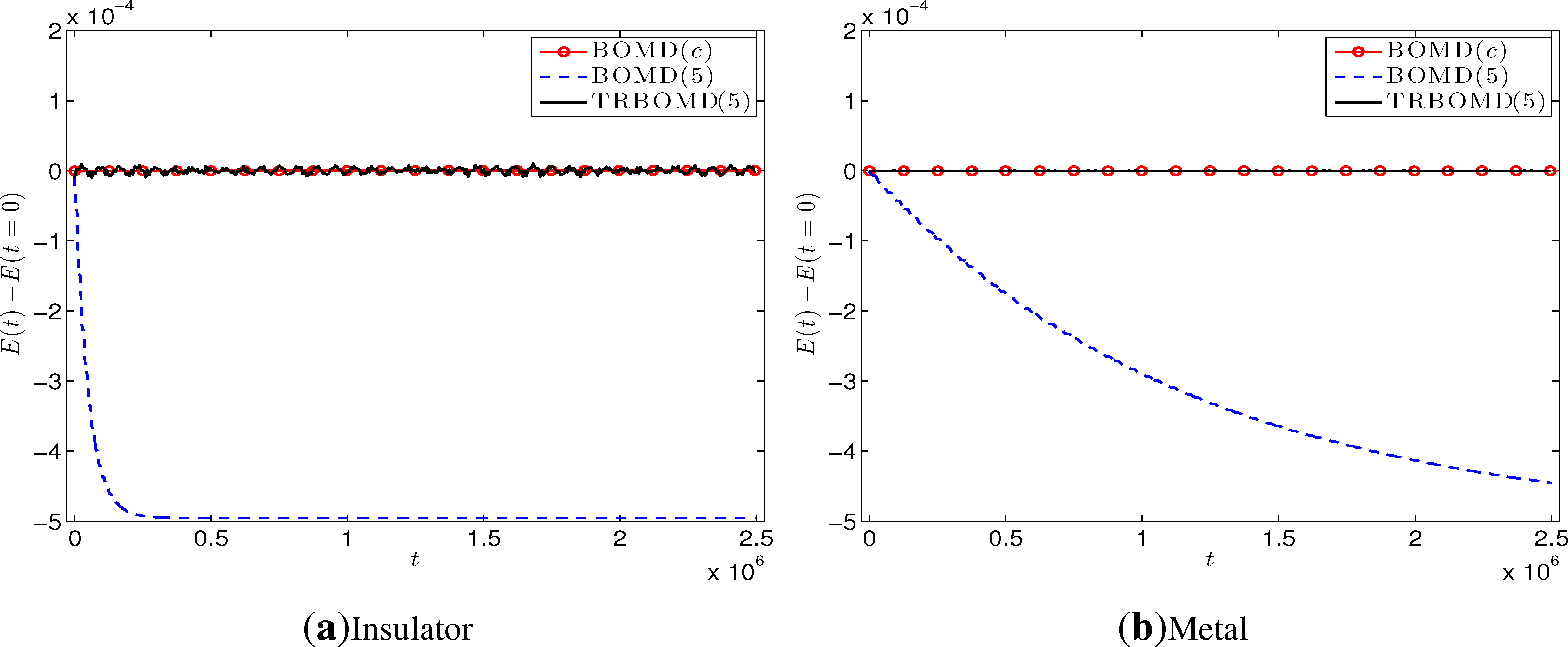
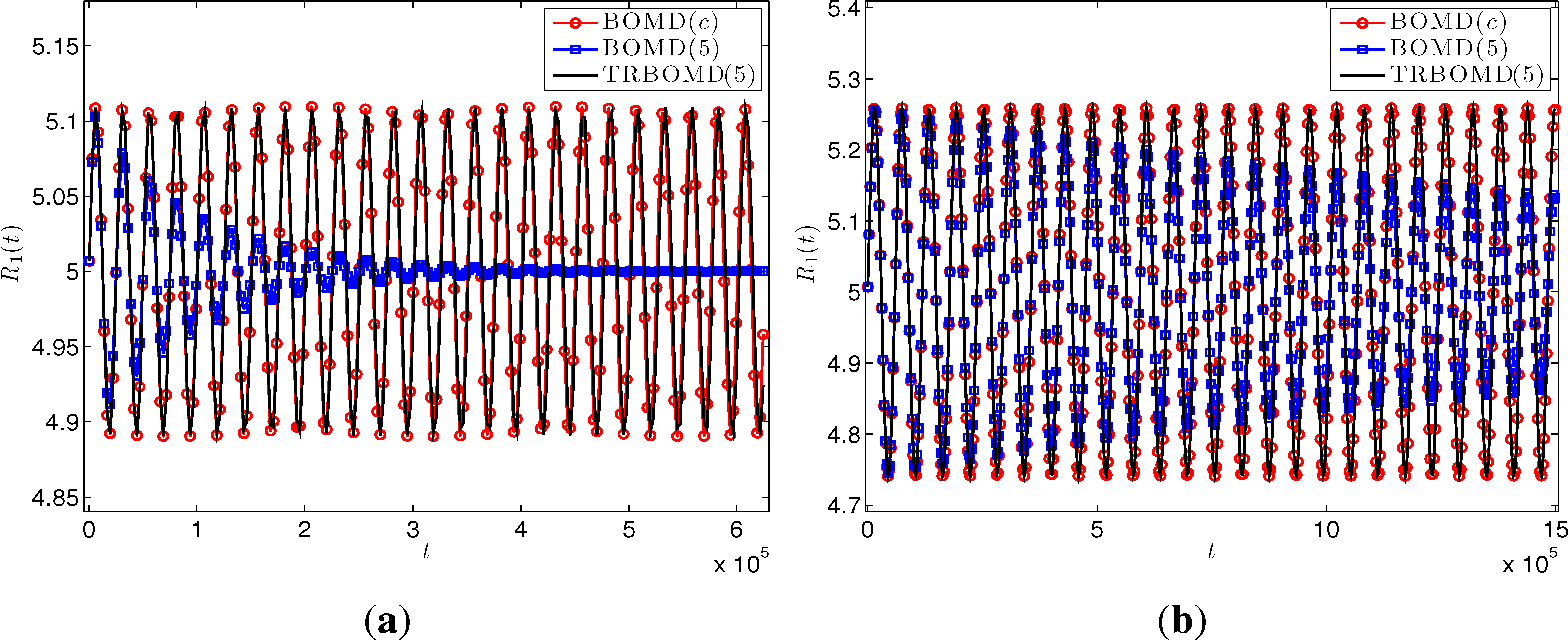
The first run is to validate the performance of TRBOMD. We set the time step Δt = 250, the artificial frequency $\omega =\frac{1}{\Delta t}=4.00\text{E}‐03$, the final time T = 2.50E+06 and employ the simple mixing with step length α= 0.3 and the Kerker preconditioner in SCF cycles. Figure 2 plots the energy drift for BOMD with the converged SCF iteration (denoted by BOMD(c)) where the tolerance is 1.00E-08; BOMD with five SCF iterations per time step (denoted by BOMD(5)) and TRBOMD with five SCF iterations per time step (denoted by TRBOMD(5)). We see clearly there that BOMD(5) produces large drift for both insulator and metal, but TRBOMD(5) does not. Actually, from

Table 1. The errors for time reversible Born-Oppenheimer molecular dynamics (TRBOMD) (n). The settings are the same as those in Figure 2, except for the number of SCF iterations.

Insulator: ΩRef = 2.51E-04, ERef = 8.66E-01
n	${\text{err}}_{\Omega }^{\text{LR}}$	${\text{err}}_{\Omega }^{\text{Hooke}}$	errĒ	${\text{err}}_R^{L^2}$	${\text{err}}_R^{L^{\infty }}$
3	−6.53E-03	−1.63E-02	−7.63E-05	2.26E-02	4.25E-02
5	−1.08E-03	−2.38E-03	−1.30E-05	1.27E-02	2.92E-02
7	−2.76E-04	−5.41E-04	−3.32E-06	3.02E-03	7.22E-03
Metal: ΩRef = 1.06E-04, E¯Ref = 5.28E-01
3	−2.65E-04	−6.92E-04	−4.36E-06	3.86E-03	8.95E-03
5	−3.65E-05	−7.31E-05	−4.44E-07	4.14E-04	9.60E-04
7	−5.24E-06	2.93E-06	−1.10E-07	1.63E-05	3.78E-05

, the relative error in the average total energy over time between TRBOMD(5) and BOMD(c) is under 1.30E-05, but BOMD(c) needs about an average of 45 SCF iterations per time step to reach the tolerance 1.00E-08. Figure 3 plots corresponding trajectory of the left-most atom during about the first 25 periods and shows that the trajectory from TRBOMD (five) almost coincides with that from BOMD (c), which is also confirmed by the data of ${\text{err}}_R^{L^2}$ and ${\text{err}}_R^{L^{\infty }}$ in Table 1. However, for BOMD(5), the atom will cease oscillation after a while. A similar phenomena occurs for other atoms. In Table 1, we present more results for TRBOMD(n) with n = 3, 5, 7. We observe there that TRBOMD(n) gives more accurate results with larger n, and ${\text{err}}_{\Omega }^{\text{Hooke}}$ has a similar behavior as n increases to ${\text{err}}_{\Omega }^{\text{LR}}$, which is in accord with our previous linear response analysis in Section 4.

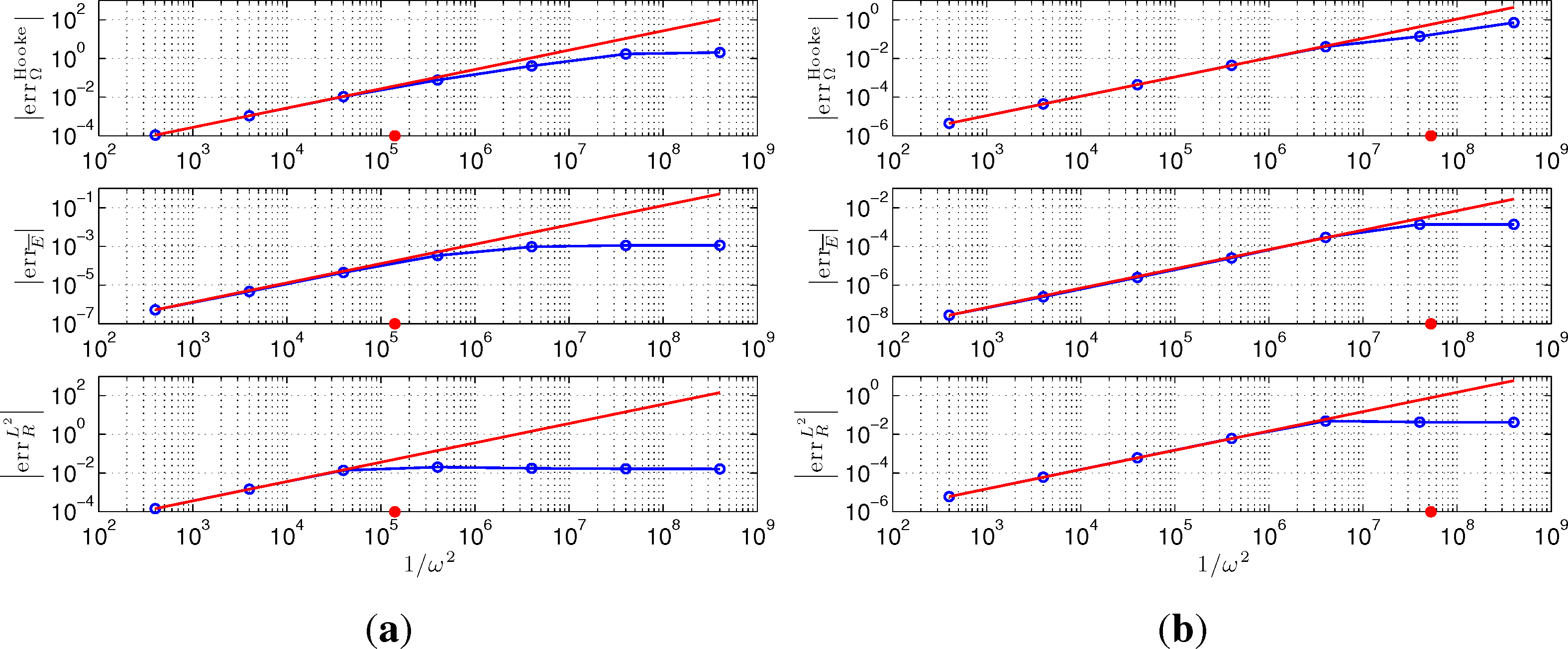
According to Equation (50), we have that ${\text{err}}_{\Omega }^{\text{LR}}$ is proportional to 1/ω² for large ω. We verify this behavior using TRBOMD(3) as an example. In this example, a smaller time step, Δt = 20, is set to allow bigger artificial frequency ω. The final time is T = 6.00E+05, and the simple mixing with α= 0.3 and the Kerker preconditioner is applied in SCF iterations. For TRBOMD (three) under these settings, we have λ_min($𝒦$) ≃ 8.81E-03 for the insulator and λ_min($𝒦$) ≃ 5.92E-01 for the metal, and thus, the critical values of (Ω^Ref)²/λ_min($𝒦$) in Equation (49) are about 7.12E-06 and 1.90E-08, respectively. We choose ω² = 2.50E-03, 2.50E-04, 2.50E-05, 2.50E-06, 2.50E-07, 2.50E-08, 2.50E-09, and plot in Figure 4 the absolute values of ${\text{err}}_{\Omega }^{\text{Hooke}}$, err_Ē, ${\text{err}}_R^{L^2}$ for TRBOMD (three) as a function of 1/ω² in logarithmic scales. When 1/ω² ≪ λ_min($𝒦$)/(Ω^Ref)², Figure 4 shows clearly that all of $\left|{\text{err}}_{\Omega }^{\text{Hooke}}\right|$,|err_Ē|, $\left|{\text{err}}_R^{L^2}\right|$ depend linearly on 1/ω². The error, ${\text{err}}_{\mathbf{R}}^{L\infty }$, has a similar behavior to ${\text{err}}_R^{L^2}$ and is skipped here for saving space.

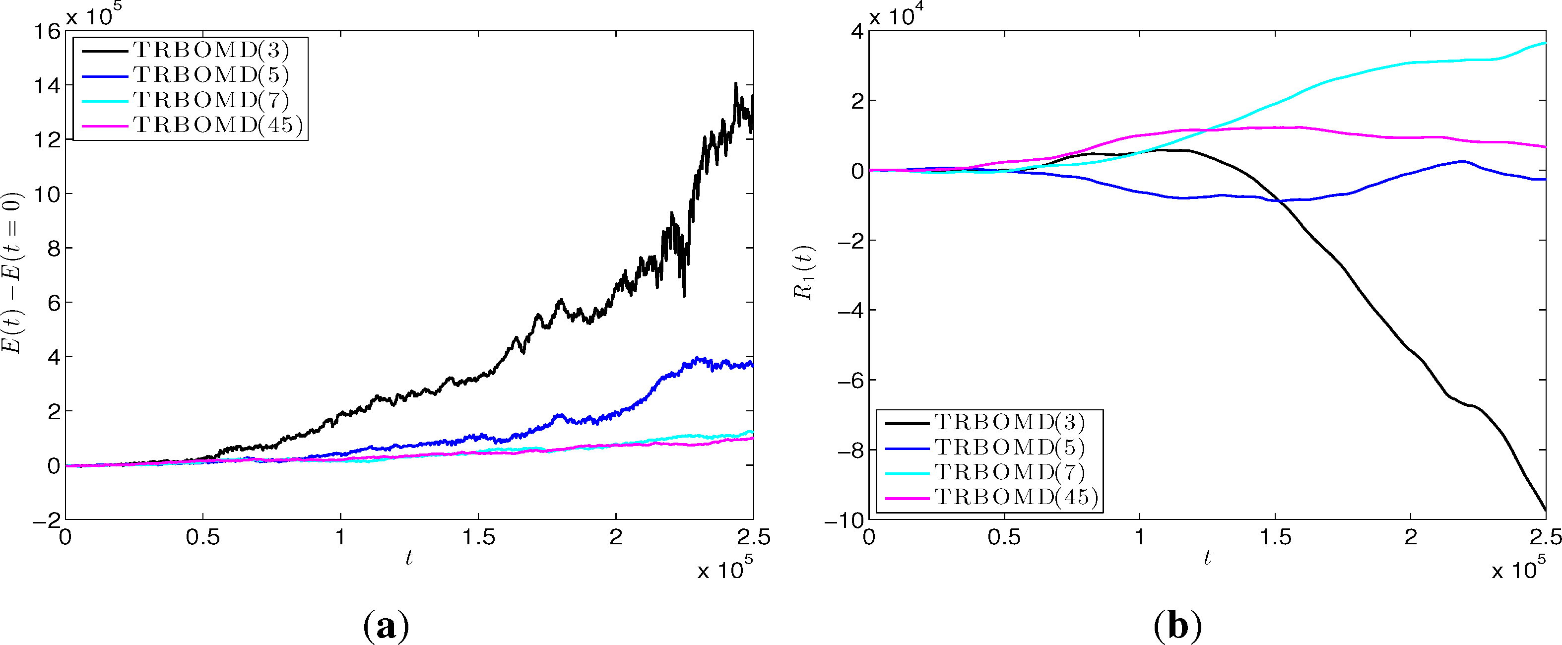
The last example illustrates the possible unstable behavior of TRBOMD when the stability condition λ_min($𝒦$) > 0 in Equation (48) is violated. Here, we take the insulator as an example and set the time step Δt = 250, the final time to 2.50E+05 and the artificial frequency $\omega =\frac{1}{\Delta t}=4.00\text{E}‐03$. The simple mixing with α= 0.3 is now applied in SCF iterations. Under these setting, we have λ_min($𝒦$) < 0, e.g., λ_min($𝒦$) = −2.42E+03 for TRBOMD (three). Figure 5a plots the energy drift for TRBOMD (n) with n = 3, 5, 7, 45. We see clearly there that TRBOMD is unstable even using 45 SCF iterations per time step (recall that BOMD (c) in the first run needs about average 45 SCF iterations per time step). Figure 5b plots the corresponding trajectory of the left-most atom and shows that the atom is driven wildly by the non-convergent SCF iteration.

5.2. Numerical Comparison between TRBOMD and CPMD

We now present some numerical examples for CPMD illustrating the difference between CPMD and TRBOMD. As we have discussed, TRBOMD is applicable to both metallic and insulting systems, while CPMD becomes inaccurate when the gap vanishes. To make this statement more concrete, we apply CPMD to the same atom chain system. We implement CPMD using a standard velocity Verlet scheme combined with RATTLEfor the orthonormality constraints [37–39].

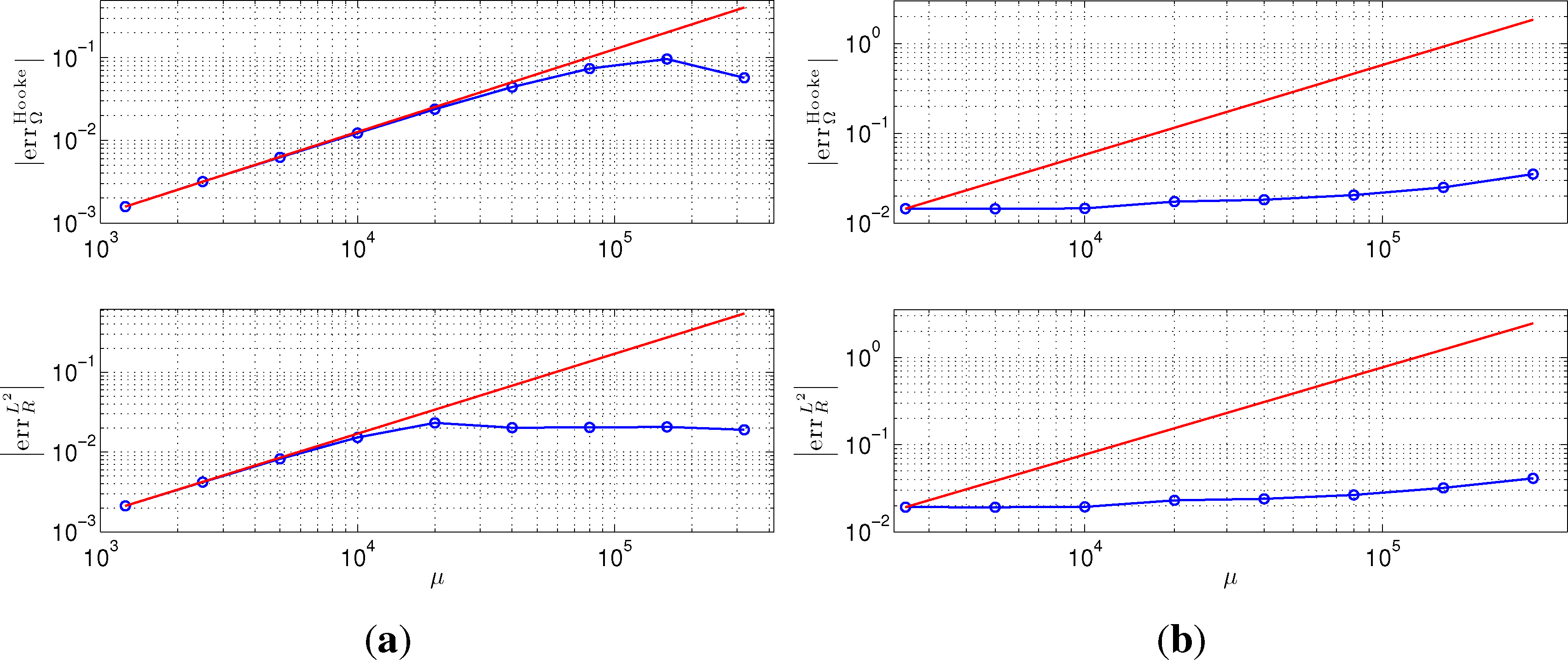
We present in Figure 6 the error of CPMD simulation for different choices of fictitious electron mass μ. We study the relative error of the phonon frequency, ${\text{err}}_{\Omega }^{\text{Hooke}}$, the relative error of the position of the left-most atom measured in L² norm, i.e., ${\text{err}}_R^{L^2}$. We observe in Figure 6a linear convergence of CPMD to the BOMD result as the parameter, μ, decreases. This is consistent with our analysis. Recall that in CPMD, μ plays a similar role as ω⁻² in TRBOMD. For the metallic example, the behavior is quite different; actually, Figure 6b shows a systematic error as μ decreases. For metallic system, as the spectral gap vanishes, the adiabatic separation between ionic and electronic degrees of freedom cannot be achieved no matter how small μ is. The adiabatic separation for TRBOMD, on the other hand, relies on the choice of an effective ρ_SCF, and hence, TRBOMD also works for a metallic system, as Figure 4 indicates.

The different behavior of CPMD for insulating and metallic systems is further illustrated by Figure 7, which shows the trajectory of the position of the left-most atom during the simulation. The phase error is apparent from the two subfigures. While the phase error decreases so that the trajectory approaches that of BOMD for the insulator in Figure 7a, the result in Figure 7b shows a systematic error for a metallic system.

6. Beyond the Linear Response Regime: Non-Equilibrium Dynamics

The discussion so far has been limited to the linear response regime so that we can make linear approximations for the degrees of freedom of both nuclei and electrons. In this case, as the system becomes linear, explicit error analysis has been given. For practical applications, we will be also interested in non-equilibrium nuclei dynamics, so that the deviation of atom positions is no longer small. In this section, we will investigate the non-equilibrium case using the averaging principle (see e.g., [40,41] for a general introduction on the averaging principle).

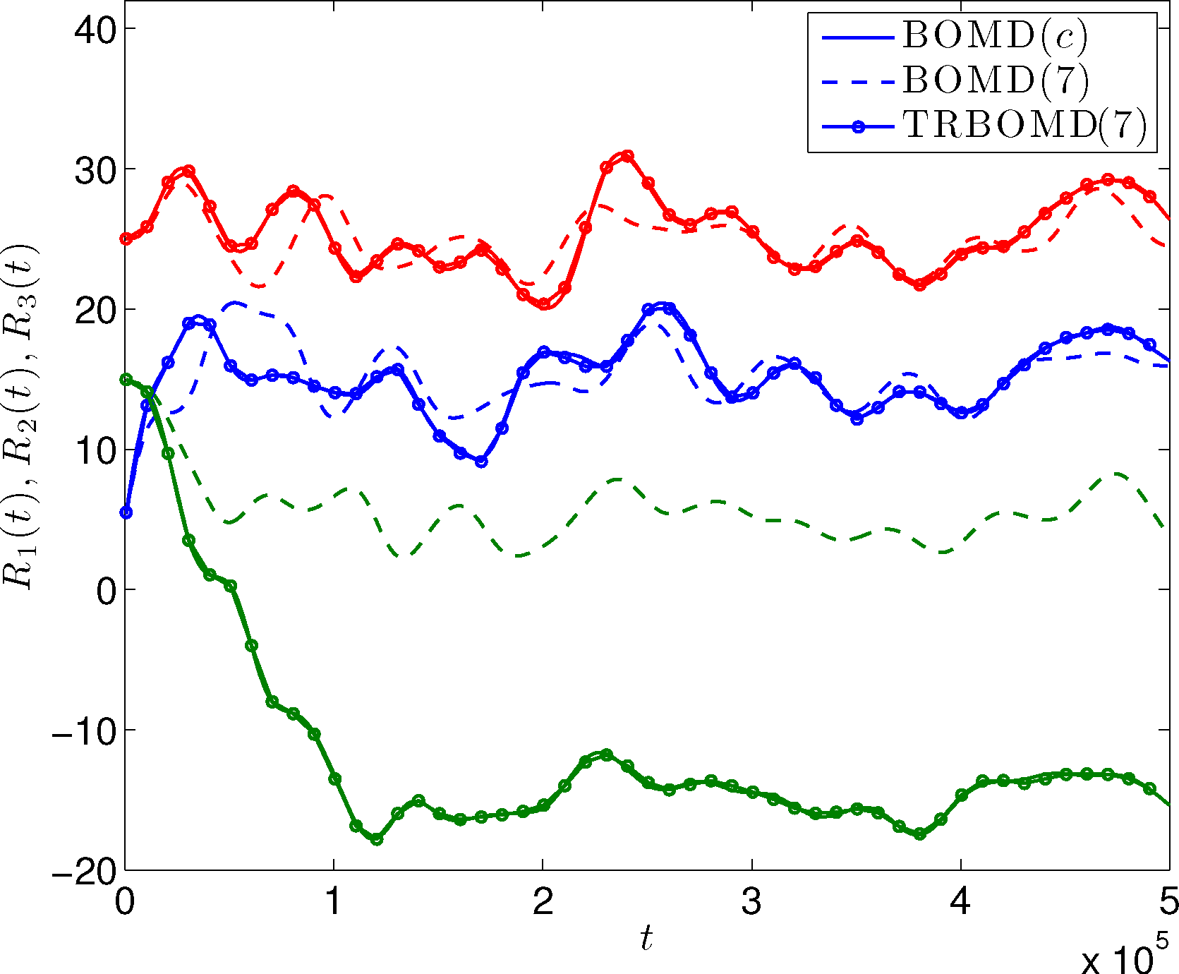
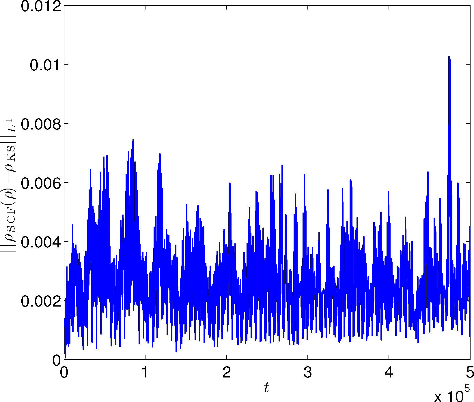
Let us first show numerically a non-equilibrium situation for the atom chain example discussed before. Initially, the 32 atoms stay at their equilibrium position. We set the initial velocity so that the left-most atom has a large velocity towards the right and other atoms have equal velocity towards the left. The mean velocity is equal to zero; so, the center of mass does not move. Figure 8 shows the trajectory of the positions of the first three atoms from the left. We observe that the results from TRBOMD agree very well with the BOMD results with convergent SCF iterations. Let us note that in the simulation, the left-most atom crosses over the second left-most atom. This happens since, in our model, we have taken a 1D analog of Coulomb interaction, the nuclei background charges are smeared out and, hence, the interaction is “soft” without hard-core repulsion. In Figure 9, we plot the difference between ρ_SCF and the converged electron density of the SCF iteration (denoted by ρ_KS) along the TRBOMD simulation. We see that the electron density used in TRBOMD stays close to the ground state electron density corresponding to the atom configuration.

To understand the performance of TRBOMD, recall that the equations of motion are given by:

$$\begin{array}{l}m{\ddot{R}}_I(t)=-\int {\rho }_{\text{SCF}}(x;\mathbf{R}(t),\rho (t))\frac{\partial V_{\text{ion}}(x;\mathbf{R}(t))}{\partial R_I}\text{d}x\\ \hspace{0.17em}\hspace{0.17em}\hspace{0.17em}\hspace{0.17em}\ddot{\rho }(x,t)={\omega }^2{\rho }_{\text{SCF}}(x;\mathbf{R}(t),\rho (t))-\rho (x,t))\end{array}$$

To satisfy the adiabatic condition (49) from the linear analysis, ω here is a large parameter. As a result, the time scales of the motions of the nuclei and of the electrons are quite different: The electronic degrees of freedom move much faster than the nuclear degrees of freedom.

Let us consider the limit, ω → ∞. In this case, we may freeze the R degree of freedom in the equation of motion for ρ, as ρ changes on a much faster time scale. To capture the two time scale behavior, we introduce a heuristic two-scale asymptotic expansion with faster time variable given by τ = ωt (with some abuse of notation):

$$R(t)=R(t)\hspace{0.17em}\hspace{0.17em}\hspace{0.17em}\text{and}\hspace{0.17em}\hspace{0.17em}\rho (x,t)=\rho (x,t,\tau )$$

(70)

and hence:

$$\ddot{\rho }(x,t)={\omega }^2{\partial }_{\tau }^2\rho (x,t,\tau )+2\omega {\partial }_{\tau }{\partial }_{t\rho }(x,t,\tau )+{\partial }_{\tau }^2\rho (x,t,\tau )$$

(71)

Therefore, to the leading order, after neglecting the terms of $𝒪$(ω⁻¹), we obtain:

$$m{\ddot{R}}_I(t)=-\int {\rho }_{\text{SCF}}(x;\mathbf{R}(t),\rho (t,\tau ))\frac{\partial V_{\text{ion}}(x;\mathbf{R}(t))}{\partial R_I}\text{d}x$$

(72)

$${\partial }_{\tau }^2\rho (x,t,\tau )={\rho }_{\text{SCF}}(x;\mathbf{R}(t),\rho (t,\tau ))-\rho (x,t,\tau )$$

(73)

For the equation of motion for ρ, note that as R only depends on t, the nuclear positions are fixed parameters in Equation (73).

To proceed, we consider the scenario that ρ (t, τ) is close to the ground state electron density corresponding to the current atom configuration, ρ^*(R(t)). We have seen from numerical examples (Figure 9) that this is indeed the case for a good choice of SCF iteration, while we do not have a proof of this in the general case. Hence, we linearize the map: ρ_SFC.

$${\rho }_{\text{SCF}}(x;\mathbf{R},\rho )={\rho }^{*}(x;\mathbf{R})+\int \frac{\delta {\rho }_{\text{SCF}}}{\delta \rho }(x,y;\mathbf{R},{\rho }^{*}(\mathbf{R}))(\rho (y)-{\rho }^{*}(y;\mathbf{R}))\text{d}y$$

(74)

and Equation (73) becomes:

$${\partial }_{\tau }^2\rho (x,t,\tau )=-𝒦(\mathbf{R})(\rho (x,t,\tau )-{\rho }^{*}(x;\mathbf{R}(t)))$$

(75)

where $𝒦$(R) is the same as in Equation (39), except it is now defined for each atom configuration, R. Let us emphasize that here we have only taken the linear approximation for the electronic degrees of freedom, while keeping the possibly nonlinear dynamics of R. This is different from the linear response regime considered before, where the nuclei motion is also linearized.

Under the stability condition (48), it is easy to see that for ρ(t, τ) satisfying Equation (75), the limit of the time average:

$$\begin{array}{l}\overline{\rho }(x;\mathbf{R}(t))=\underset{T\to \infty }{\text{lim}}\frac{1}{T}{\int }_0^T{\rho }_{\text{SCF}}(x;\mathbf{R}(t),\rho (t,\tau ))\text{d}\tau \\ \hspace{0.17em}\hspace{0.17em}\hspace{0.17em}\hspace{0.17em}\hspace{0.17em}\hspace{0.17em}\hspace{0.17em}\hspace{0.17em}\hspace{0.17em}\hspace{0.17em}\hspace{0.17em}\hspace{0.17em}\hspace{0.17em}\hspace{0.17em}\hspace{0.17em}\hspace{0.17em}\hspace{0.17em}\hspace{0.17em}\hspace{0.17em}\hspace{0.17em}\hspace{0.17em}\hspace{0.17em}\approx {\rho }^{*}(x;\mathbf{R}(t))+\int \frac{\delta {\rho }_{\text{SCF}}}{\delta \rho }(x,y;\mathbf{R},{\rho }^{*}(\mathbf{R}))\left(\underset{T\to \infty }{\text{lim}}\frac{1}{T}{\int }_0^T\rho (y;t,\tau )-{\rho }^{*}(y;\mathbf{R}(t))\text{d}\tau \right)\text{d}y\\ \hspace{0.17em}\hspace{0.17em}\hspace{0.17em}\hspace{0.17em}\hspace{0.17em}\hspace{0.17em}\hspace{0.17em}\hspace{0.17em}\hspace{0.17em}\hspace{0.17em}\hspace{0.17em}\hspace{0.17em}\hspace{0.17em}\hspace{0.17em}\hspace{0.17em}\hspace{0.17em}\hspace{0.17em}\hspace{0.17em}\hspace{0.17em}\hspace{0.17em}\hspace{0.17em}\hspace{0.17em}={\rho }^{*}(x;\mathbf{R}(t))\end{array}$$

(76)

Take the average of Equation (72) in τ, we have:

$$m{\ddot{R}}_I(t)=-\int \overline{\rho }(x;\mathbf{R}(t))\frac{\partial V_{\text{ion}}(x;\mathbf{R}(t))}{\partial R_I}\text{d}x$$

(77)

Because of Equation (76), the above dynamics is given by:

$$m{\ddot{R}}_I(t)=-\int {\rho }^{*}(x;\mathbf{R}(t))\frac{\partial V_{\text{ion}}(x;\mathbf{R}(t))}{\partial R_I}\text{d}x$$

(78)

which agrees with the equation of the motion of atoms in BOMD. As we have neglected $𝒪$(ω⁻¹) terms in the averaging, the difference in the trajectory of BOMD and TRBOMD is on the order of $𝒪$(ω⁻¹) for finite ω.

Remark. If we do not make the linear approximation for the electronic degree of freedom, as the map, ρ_SCF, is quite nonlinear and complicated, the analysis of the long time (in τ) behavior of Equation (73) is not as straightforward. In particular, it is not clear to us whether the limit:

$$\overline{\rho }(x;\mathbf{R}(t))=\underset{T\to \infty }{\text{lim}}\frac{1}{T}{\int }_0^T{\rho }_{\text{SCF}}(x;\mathbf{R}(t),\rho (t,\tau ))\text{d}\tau$$

(79)

exists or how close the limit is to ρ^*(x; R(t)) in a fully nonlinear regime. One particular difficulty lies in the fact that unlike BOMD or CPMD, we do not have a conserved Lagrangian for the TRBOMD. Actually, it is easy to construct a much simplified analog of Equation (73), the average of which is different from ρ^*. For example, if we consider the following analog, which only has one degree of freedom, ξ:

$$\ddot{\xi }=\left(\xi /2+a{\xi }^2\right)-\xi$$

(80)

where (ξ/2 + aξ²) is the analog of ρ_SCF, here, and a > 0 is a small parameter, which characterizes the nonlinearity of the map. Note that:

$$\ddot{\xi }=-\xi /2+a{\xi }^2=-{\partial }_{\xi }\left({\xi }^2/4-a{\xi }^3/3\right)$$

(81)

The motion of ξ is equivalent to the motion of a particle in an anharmonic potential. It is clear that if, initially, ξ(0) ≠ 0, the long time average of ξ will not be zero. Furthermore, if, initially, ξ(0) is too large, the orbit is not closed (ξ escapes the well around ξ = 0). If phenomena similar to this occur for a general ρ_SCF, then even in the limit, ω → ∞, there will be a systematic uncontrolled bias between BOMD and TRBOMD. This is in contrast with Car-Parrinello molecular dynamics, which agrees with BOMD in the limit fictitious mass going to zero (μ → 0) if the adiabatic condition holds.

As a result of this discussion, in practice, when we apply TRBOMD to a particular system, we need to be cautious whether the electronic degree of freedom remains around the converged Kohn-Sham electron density, which is not necessarily guaranteed (in contrast to CPMD for systems with gaps).

7. Conclusions

The recently developed time reversible Born-Oppenheimer molecular dynamics (TRBOMD) scheme provides a promising way for reducing the number of self-consistent field (SCF) iterations in molecular dynamics simulation. By introducing auxiliary dynamics to the initial guess of the SCF iteration, TRBOMD preserves the time-reversibility of the NVE dynamics, both at the continuous and at the discrete level, and exhibits improved long time stability over the Born-Oppenheimer molecular dynamics with the same accuracy. In this paper we analyze, for the first time, the accuracy and the stability of the TRBOMD scheme, and our analysis is verified through numerical experiments using a one-dimensional density functional theory (DFT) model without exchange correlation potential. The validity of the stability condition in TRBOMD is directly associated with the quality of the SCF iteration procedure. In particular, we demonstrate in the case in which the SCF iteration procedure is not very accurate, the stability condition can be violated, and TRBOMD becomes unstable. We also compare TRBOMD with the Car-Parrinello molecular dynamics (CPMD) scheme. CPMD relies on the adiabatic evolution of the occupied electron states, and therefore, CPMD works better for insulators than for metals. However, TRBOMD may be effective for both insulating and metallic systems. The present study is restricted to the NVE system and to simplified DFT models. Moreover, the analysis in the present work is mainly focused on the accuracy of trajectories and harmonic frequencies in the perturbation regime. However, in practice, the more important question is how the introduced artificial dynamics influence static properties, like distribution functions, and the most critical capability is to reproduce the correct distribution functions. The performance of TRBOMD for the NVT system and for realistic DFT systems with emphasis on the accuracy of static properties will be our future work.

References

- Marx, D.; Hutter, J. Ab initio molecular dynamics: Theory and implementation. Mod. Methods Algorithms Quantum Chem 2000, 1, 301–449. [Google Scholar]
- Kirchner, B.; di Dio, P.J.; Hutter, J. Real-world predictions from ab initio molecular dynamics simulations. Top. Curr. Chem 2012, 307, 109–153. [Google Scholar]
- Payne, M.C.; Teter, M.P.; Allen, D.C.; Arias, T.A.; Joannopoulos, J.D. Iterative minimization techniques for ab initio total energy calculation: Molecular dynamics and conjugate gradients. Rev. Mod. Phys 1992, 64, 1045–1097. [Google Scholar]
- Deumens, E.; Diz, A.; Longo, R.; Öhrn, Y. Time-dependent theoretical treatments of the dynamics of electrons and nuclei in molecular systems. Rev. Mod. Phys 1994, 66, 917–983. [Google Scholar]
- Tuckerman, M.E.; Ungar, P.J.; von Rosenvinge, T.; Klein, M.L. Ab initio molecular dynamics simulations. J. Phys. Chem 1996, 100, 12878–12887. [Google Scholar]
- Parrinello, M. From silicon to RNA: The coming of age of ab initio molecular dynamics. Solid State Commun 1997, 102, 107–120. [Google Scholar]
- Marx, D.; Hutter, J. Ab initio Molecular Dynamics: Basic Theory and Advanced Methods; Cambridge University Press: Cambridge, UK, 2009. [Google Scholar]
- Hohenberg, P.; Kohn, W. Inhomogeneous electron gas. Phys. Rev 1964, 136, B864–B871. [Google Scholar]
- Kohn, W.; Sham, L. Self-consistent equations including exchange and correlation effects. Phys. Rev 1965, 140, A1133–A1138. [Google Scholar]
- Remler, D.K.; Madden, P.A. Molecular dynamics without effective potentials via the Car-Parrinello approach. Mol. Phys 1990, 70, 921–966. [Google Scholar]
- Car, R.; Parrinello, M. Unified approach for molecular dynamics and density-functional theory. Phys. Rev. Lett 1985, 55, 2471–2474. [Google Scholar]
- Pastore, G.; Smargiassi, E.; Buda, F. Theory of ab initio molecular-dynamics calculations. Phys. Rev. A 1991, 44, 6334–6347. [Google Scholar]
- Bornemann, F.A.; Schütte, C. A mathematical investigation of the Car-Parrinello method. Numer. Math 1998, 78, 359–376. [Google Scholar]
- Niklasson, A.M.N.; Tymczak, C.J.; Challacombe, M. Time-reversible Born-Oppenheimer molecular dynamics. Phys. Rev. Lett 2006, 97, 123001:1–123001:4. [Google Scholar]
- Niklasson, A.M.N.; Tymczak, C.J.; Challacombe, M. Time-reversible ab initio molecular dynamics. J. Chem. Phys 2007, 126, 144103:1–144103:9. [Google Scholar]
- Niklasson, A.M.N. Extended Born-Oppenheimer molecular dynamics. Phys. Rev. Lett 2008, 100, 123004:1–123004:4. [Google Scholar]
- Niklasson, A.M.N.; Steneteg, P.; Odell, A.; Bock, N.; Challacombe, M.; Tymczak, C.J.; Holmström, E.; Zheng, G.; Weber, V. Extended Lagrangian Born-Oppenheimer molecular dynamics with dissipation. J. Chem. Phys 2009, 130, 214109. [Google Scholar] [CrossRef]
- Niklasson, A.M.N.; Cawkwell, M.J. Fast method for quantum mechanical molecular dynamics. Phys. Rev. B 2012, 86, 174308:1–174308:12. [Google Scholar]
- Hairer, E.; Lubich, C.; Wanner, G. Geometric Numerical Integration, 2nd ed.; Springer: Berlin/Heidelberg, Germany, 2006. [Google Scholar]
- McLachlan, R.I.; Perlmutter, M. Energy drift in reversible time integration. J. Phys. A: Math. Gen 2004, 37, L593–L598. [Google Scholar]
- Kolafa, J. Time-reversible always stable predictor-corrector method for molecular dynamics of polarizable molecules. J. Comput. Chem 2004, 25, 335–342. [Google Scholar]
- Kühne, T.D.; Krack, M.; Mohamed, F.R.; Parrinello, M. Efficient and accurate Car-Parrinello-like approach to Born-Oppenheimer molecular dynamics. Phys. Rev. Lett 2007, 98, 066401:1–066401:4. [Google Scholar]
- Dai, J.; Yuan, J. Large-scale efficient Langevin dynamics, and why it works. EPL 2009, 88, 20001. [Google Scholar] [CrossRef]
- Hutter, J. Car-Parrinello molecular dynamics. WIREs Comput. Mol. Sci 2012, 2, 604–612. [Google Scholar]
- Anderson, D.G. Iterative procedures for nonlinear integral equations. J. Assoc. Comput. Mach 1965, 12, 547–560. [Google Scholar]
- Pulay, P. Convergence acceleration of iterative sequences: The case of SCF iteration. Chem. Phys. Lett 1980, 73, 393–398. [Google Scholar]
- Johnson, D.D. Modified Broyden’s method for accelerating convergence in self-consistent calculations. Phys. Rev. B 1988, 38, 12807–12813. [Google Scholar]
- Kerker, G.P. Efficient iteration scheme for self-consistent pseudopotential calculations. Phys. Rev. B 1981, 23, 3082–3084. [Google Scholar]
- Lin, L.; Yang, C. Elliptic preconditioner for accelerating self consistent field iteration in Kohn-Sham density functional theory. SIAM J. Sci. Comput 2013, 35, S277–S298. [Google Scholar]
- McLachlan, R.I.; Atela, P. The accuracy of symplectic integrators. Nonlinearity 1992, 5, 541–562. [Google Scholar]
- Adler, S.L. Quantum theory of the dielectric constant in real solids. Phys. Rev 1962, 126, 413–420. [Google Scholar]
- Wiser, N. Dielectric constant with local field effects included. Phys. Rev 1963, 129, 62–69. [Google Scholar]
- Blöchl, P.E.; Parrinello, M. Adiabaticity in first-principles molecular dynamics. Phys. Rev. B 1992, 45, 9413–9416. [Google Scholar]
- Tangney, P.; Scandolo, S. How well do Car-Parrinello simulations reproduce the Born-Oppenheimer surface? Theory and examples. J. Chem. Phys 2002, 116, 14–24. [Google Scholar]
- Tangney, P. On the theory underlying the Car-Parrinello method and the role of the fictitious mass parameter. J. Chem. Phys 2006, 124, 044111:1–044111:14. [Google Scholar]
- Solovej, J.P. Proof of the ionization conjecture in a reduced Hartree-Fock model. Invent. Math 1991, 104, 291–311. [Google Scholar]
- Ryckaert, J.P.; Ciccotti, G.; Berendsen, H.J.C. Numerical integration of the cartesian equations of motion of a system with constraints: Molecular dynamics of n-alkanes. J. Comput. Phys 1977, 23, 327–341. [Google Scholar]
- Ciccotti, G.; Ferrario, M.; Ryckaert, J.P. Molecular dynamics of rigid systems in cartesian coordinates: A general formulation. Mol. Phys 1982, 47, 1253–1264. [Google Scholar]
- Andersen, H.C. Rattle: A “velocity” version of the Shake algorithm for molecular dynmiacs calculations. J. Comput. Phys 1983, 52, 24–34. [Google Scholar]
- E, W. Principles of Multiscale Modeling; Cambridge University Press: Cambridge, UK, 2011. [Google Scholar]
- Pavliotis, G.; Stuart, A. Multiscale Methods: Averaging and Homogenization; Springer: Berlin/Heidelberg, Germany, 2008. [Google Scholar]