Time Integrators for Molecular Dynamics

Abstract
: This paper invites the reader to learn more about time integrators for Molecular Dynamics simulation through a simple MATLAB implementation. An overview of methods is provided from an algorithmic viewpoint that emphasizes long-time stability and finite-time dynamic accuracy. The given software simulates Langevin dynamics using an explicit, second-order (weakly) accurate integrator that exactly reproduces the Boltzmann-Gibbs density. This latter feature comes from adding a Metropolis acceptance-rejection step to the integrator. The paper discusses in detail the properties of the integrator. Since these properties do not rely on a specific form of a heat or pressure bath model, the given algorithm can be used to simulate other bath models including, e.g., the widely used v-rescale thermostat.1. Introduction
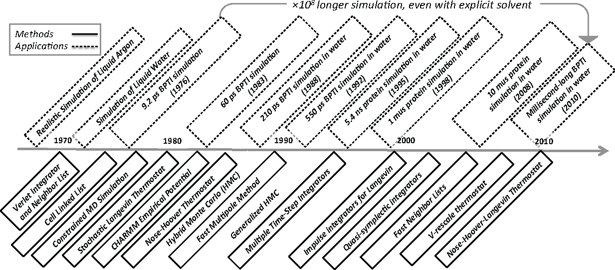
Molecular Dynamics (MD) simulation refers to the time integration of Hamilton’s equations often coupled to a heat or pressure bath [1–5]. From its early use in computing equilibrium dynamics of homogeneous molecular systems [6–13] and pico- to nano-scale protein dynamics [14–23], the method has evolved into a general purpose tool for simulating statistical properties of heterogeneous molecular systems [24]. Accessible time horizons have increased remarkably: the time line in Figure 1 attempts to capture this nearly billion-fold improvement in capability over the last forty or so years. To put this speedup in perspective, though, computing power has increased by about eight powers of ten over this time period as predicted by Moore’s law.
To be clear, the selection of applications and methods shown in Figure 1 is not comprehensive and heavily biased towards the specific ideas and methods that inform this paper. The applications highlighted are simulations of liquid argon [6], water [11], protein dynamics without solvent [14,15] and biopolymer dynamics with solvent [25–31]. The methods include the following “upgrades” to MD simulation: Verlet integrator and neighbor lists [7], cell linked list [32], the SHAKE integrator for constraints [33], stochastic heat baths via Langevin dynamics [34,35], a library of empirical potentials [36], a deterministic heat bath via Nosé-Hoover dynamics [37,38], the fast multipole method [39], multiple time steps [40], splitting methods for Langevin dynamics [41–43], quasi-symplectic integrators [44,45], (fast) combined neighbor and cell lists [46], the v-rescale thermostat [47] and the stochastic Nosé-Hoover Langevin thermostat [48–50].
Near future applications of MD simulation include micro- to milli-scale simulations of biomolecular processes, like protein folding, ligand binding, membrane transport and biopolymer conformational changes [51–53]. In addition, atomistic MD simulations are used more sparingly in multiscale models [54–58] and rare event simulation, such as the finite temperature string method and milestoning [59–62]. Given this continuous development and generalization of MD, it is not a stretch to suppose that MD will play a transformative role in medicine, technology and education in the twenty-first century.
In its standard form, the method inputs a random initial condition, physical and numerical parameters and outputs a long discrete path of the molecular system. Statistical quantities, like velocity correlation or mean radius of gyration, are usually computed online, i.e., as points along this trajectory are produced. MD simulation is built atop a cheap forward Euler-like integrator that requires only a single interactomic force field evaluation per step. Even though MD seems straightforward, software implementations of MD are typically optimized for performance [36,63,64], and as a side effect, make it cumbersome for non-experts to learn and modify.
Also, besides this issue, due to the interplay between stochastic Brownian and molecular forces, infinitely long trajectories of existing MD integrators do not have the right distribution. What happens is that the Brownian force can cause the integrator to enter regions where its approximation to the molecular force is inaccurate and possibly destabilizing. In the latter case, the approximation spends a disproportionate amount of time at higher energies, and thus, the invariant measure of the approximation, if it even exists, is not correct. This phenomenon is a well-known shortcoming of explicit integrators for nonlinear diffusions [65–69].
Recently, a probabilistic approach was proposed to solve this problem, which questions the notion that Monte Carlo methods and MD have different aims: the former strictly samples probability distributions, and the latter estimates dynamics. The basic idea is to combine a standard MD integrator with a Metropolis-Hastings algorithm targeted to the Boltzmann-Gibbs distribution [70–72]. Because the scheme is a Monte Carlo method, it exactly preserves the desired distribution [71,72]. This property implies numerical stability over long-time simulations. However, the price to be paid for this stability is a loss of accuracy whenever a move is rejected and some overhead in evaluating the Metropolis acceptance-rejection step. Still, a Metropolized integrator is dynamically accurate on finite-time intervals [72,73], and so, even though a Metropolized integrator involves a Monte Carlo step, its aim and philosophy are very different from Monte Carlo methods, whose only goal is to sample a target distribution with no concern for the dynamics [71,74–82]. In principle, this approach offers a simple alternative to costly implicit integrators, but are Metropolized integrators ready for daily use in MD simulation? The answer to this question is unclear, since this approach is new and has not been tested on enough examples.
Motivated by these issues, this paper builds a software system for MD simulation with a Metropolis step built in and applies it to a homogeneous molecular system. The algorithm and its properties are introduced in a step-by-step fashion. In particular, we show that the integrator is second-order weakly accurate on finite-time intervals and converges to the Boltzmann-Gibbs distribution in the long-time limit. The software version of the algorithm is written in the latest version of MATLAB with plenty of comments, variables that are descriptively named and operations that can be easily translated into mathematical expressions [83]. Since MATLAB is widely available, this design ensures that the software will be easy-to-use and cross-platform. The following MATLAB-specific file formats will be used.
(F1) MATLAB script and function files are written in the MATLAB language and can be run from the MATLAB command line without ever compiling them.
(F2) MATLAB executable (MEX) files are written in the “C” language and compiled using the MATLAB mex function. The resulting executable is comparable in efficiency to a “C” code and can be called directly from the MATLAB command line. We will use MEX-files for performance-critical routines [84].
(F3) MATLAB binary (MAT) files will be used to store simulation data.
The paper is organized as follows. We begin with an overview of integrators that have been proposed in MD simulation in Section 2. We explain how to Metropolize each of these schemes to make them long-time stable in Section 3, and as an application, we use a Metropolized scheme to generate a long trajectory of a Lennard-Jones fluid in Section 4. Generalizations of corrected MD integrators to other molecular models are discussed in Section 5. The paper closes by discussing some potential pitfalls in high dimension and tricks to get the integrator to scale well in Section 6.
2. Algorithmic Introduction to Time Integrators for MD Simulation
For pedagogical reasons, we will start with Langevin dynamics of a system of N molecules. Then, we show in Section 5 how to simulate more general models of molecular systems. Denote by mj > 0 and qj the mass and position of the j-th molecule, respectively. The governing Langevin equation is given by:
The bath-free dynamics is a Hamiltonian system with the following Hamiltonian energy function:
Let h be a given time step size and m = diag(m1, · · ·, mN). Let (Q0, P0) denote the position and momentum of the molecular system at time t > 0. The simplest approximation to Equation (1) is a forward Euler discretization or Euler-Maruyama scheme [85] that computes an updated position and momentum (Q1, P1) at t + h using:
An improvement to the forward Euler method is the following two-step scheme:
Second-order accurate schemes that generalize the Velocity Verlet integrator to Langevin dynamics were proposed in a sequence of papers [42–44,87,88]. Here, we mention two of these schemes that are both Strang splittings of Equation (1). The first was proposed by Ricci and Ciccotti [42] and consists of the following sub-steps:
A related, but different, splitting method was proposed by Bussi and Parinello in [43] and is given by:
Since the Velocity Verlet integrator does not exactly preserve energy, the composition above does not exactly preserve the stationary distribution with density in Equation (3). In [90], it was shown that if the derivatives of the potential are all bounded, the Bussi and Parinello integrator possesses an invariant measure that is (h2) close to the Boltzmann-Gibbs distribution. In this same context, the leading order error term in the integrator’s approximation to the invariant measure was explicitly determined [91]. Technically speaking, however, these results do not directly apply to MD simulation, since real MD simulation involves potentials whose derivatives are unbounded, e.g., Lennard-Jones forces. As a consequence of this irregularity in the force fields and discretization error, explicit schemes, like this one, may either not detect features of the potential energy properly, which leads to unnoticed, but large errors in dynamic quantities such as the mean first passage time, or may mishandle soft- or hard-core potentials, which leads to numerical instabilities; see the numerical examples in [92]. These numerical artifacts motivate adding a Metropolis accept/refusal sub-step to the integrator. In the next section, we show how to Metropolize all of the MD integrators presented in this section. In Section 5, we explain how to generalize the Metropolis-corrected Bussi and Parinello algorithm to a larger class of diffusion processes.
3. Metropolis-Corrected MD Integrators
Here, we show how to add a Metropolis acceptance-rejection step to a BBK-type scheme and the Bussi and Parinello splitting scheme and then precisely state the properties of these integrators. We start with a detailed description of each algorithm. Both algorithms require evaluating the acceptance probability given by the usual Metropolis ratio:
Algorithm 3.1 (First-order BBK-type integrator). Given the current state (Q0, P0) at time t, the algorithm proposes a new state ( , ) at time t + h for some time step h > 0 via:
The momenta of the molecules gets reversed if a move is rejected in Step 2 of Algorithm 3.1. This momentum flip is necessary for the algorithm to preserve the correct stationary distribution [70,71], but results in an O(1) error in dynamics. High acceptance rates are therefore needed to ensure that the time lag between successive rejections is frequently long enough for the approximation to capture the desired dynamics. Since the acceptance rate in Equation (4) is related to how well the Verlet integrator in (Step 1) preserves energy after a single step, this rejection rate is O(h3). Thus, in practice, we find that the time step required to obtain a sufficiently high acceptance rate is often automatically fulfilled by a time step that sufficiently resolves the desired dynamics. Each step of this algorithm requires: evaluating the atomic force field once in the third equation of (Step 1), generating a Bernoulli random variable with parameter α in (Step 2) and generating an n-dimensional Gaussian vector in (Step 3). We stress that (Step 2) in Algorithm 3.1 is all that is needed to get MD integrators to exactly preserve the Boltzmann-Gibbs density in Equation (3).
Next, we show how to Metropolize the Bussi and Parinello splitting integrator.
Algorithm 3.2 (Second-order Bussi and Parinello integrator). Let ξ, η ∈ ℝn be two independent Gaussian random vectors with mean zero and covariance 𝔼(ξiξj) = 𝔼 (ηiηj) = δij. Given a time step size h and the current state (Q0, P0) at time t, the algorithm takes a half-step of the heat bath dynamics:
This algorithm requires generating two independent n-dimensional Gaussian vectors per step. Thus, it is more costly than Algorithm 3.1. However, the advantage of doing this is that the resulting Metropolis corrected algorithm is second-order weakly accurate, as the following Proposition states.
Proposition 3.3. Let (Qn, Pn) represent the numerical approximation produced by Algorithm 3.2 at time nh with the same initial condition as the true solution: (Q0, P0) = (q(0), p(0)). For every time interval T > 0 and for suitable observables f(q, p), there exists a C(T) > 0, such that:
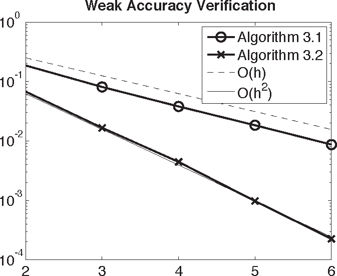
This accuracy concept is sufficient for computing means and correlation functions at finite-time and equilibrium correlations. Figure 2 verifies this Proposition by checking the weak accuracy of Algorithms 3.1 and 3.2 on a harmonic oscillator test problem.
To be specific, Figure 2 plots the weak accuracy of the Metropolis-corrected MD integrators with respect to the true solution of the Langevin dynamics of a harmonic oscillator: q̇(t) = p(t), , with initial condition q(0) = 1.0, p(0) = 0. The time steps tested are h = 2−n, where n is given on the x-axis. The quantity monitored for the error is the estimate of 𝔼(q(1)2 + p(1)2) = 1.699445410 computed analytically. The dashed and solid curves are the graphs of 2−n(= h) and 2−2n(= h2) versus n, respectively.
Proof. The desired single-step error estimate can be obtained from an application of the triangle inequality:
For completeness sake, we also provide a statement that both algorithms are ergodic.
Proposition 3.4. Let (Qn, Pn) be the numerical approximation produced by Algorithms 3.1 or 3.2 at time nh. Then, for suitable observables f(q, p):
A proof of this Proposition can be found in [72].
4. Application to Lennard-Jones Fluid
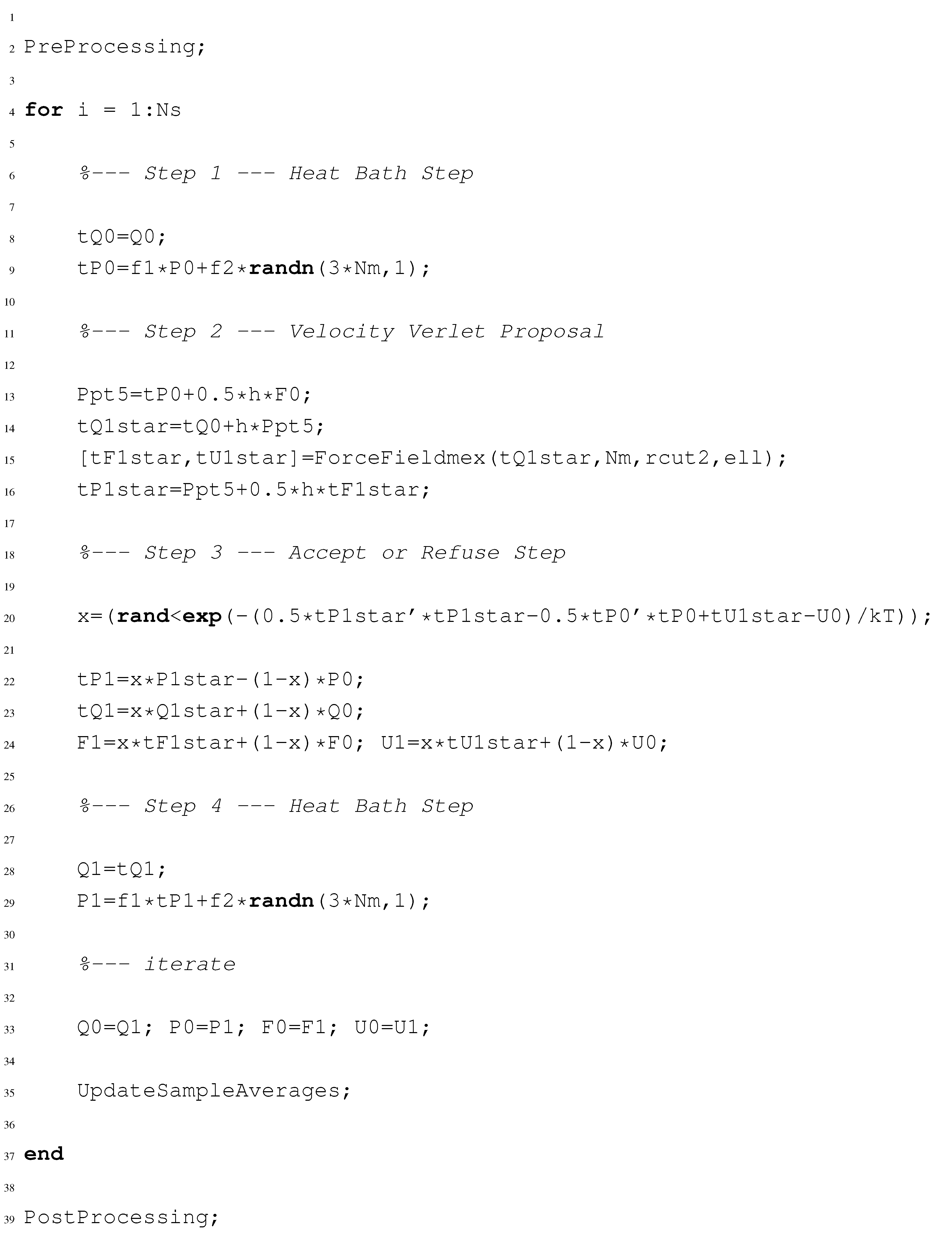
Listing 1 translates Algorithm 3.2 into the MATLAB language. Intrinsically defined MATLAB functions appear in boldface. The algorithm uses MATLAB’s built in random number generators to carry out Step 1, Step 3 and Step 4. In particular, the Bernoulli random variable, x, in Step 3 is generated in Line 20, and the Gaussian vectors in Step 1 and Step 4 are generated on Line 9 and Line 29, respectively. In addition to updating the positions and momenta of the system, the program also stores the previous value of the potential energy and force, so that the force and potential energy is evaluated in Line 15 just once per simulation step. This evaluation calls a MEX function, which inputs the current position of the molecular system and outputs the force field and potential energy at that position. We use a MEX function, because the atomistic force field evaluation cannot be easily vectorized and is, by far, the most computationally demanding step in MD. The PreProcessing script file called in Line 2 defines the physical and numerical parameters, sets the initial condition and allocates space for storing simulation data. Sample averages are updated as new points on the trajectory are produced in the UpdateSampleAverages script file invoked in Line 35. Finally, the outputs produced by the algorithm are handled by the PostProcessing script file in Line 39.
Let us consider a concrete example: a Lennard-Jones fluid that consists of N identical atoms [1–3]. The configuration space of this system is a fixed cubic box with periodic boundary conditions. The distance between the i-th and j-th particle is defined according to the minimum image convention, which states that the distance between qi and qj in a cubic box of length ℓ is:


Here, f(r) = 4(1/r12 − 1/r6) and rc is the cutoff radius, which is bounded above by the size of the simulation box; and we have used dimensionless units to describe this system, where energy is rescaled by the depth of the Lennard-Jones potential energy and length by the point where the potential energy is zero. The error introduced by the truncation in Equation (10) is proportional to the density of the molecular system and can be made arbitrarily small by selecting the cutoff distance to be sufficiently large. A direct evaluation of the potential force, ∇U(q), scales like O(N2), and typically dominates the total computational cost. In practice, neighbor/cell lists, also called Verlet lists, are used in order to obtain a force evaluation that scales linearly with system size. Since the system we consider will have just a few hundred atoms, there is, however, little advantage to using these data structures, or using a fast force field evaluation, and thus, ForceFieldmex evaluates the force and energy using a sum over all particle pairs.
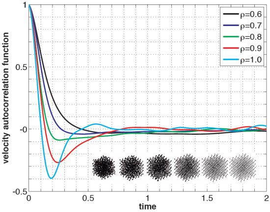
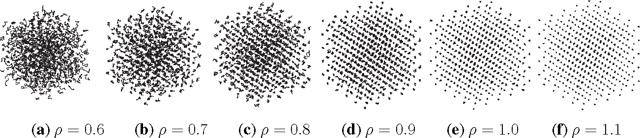
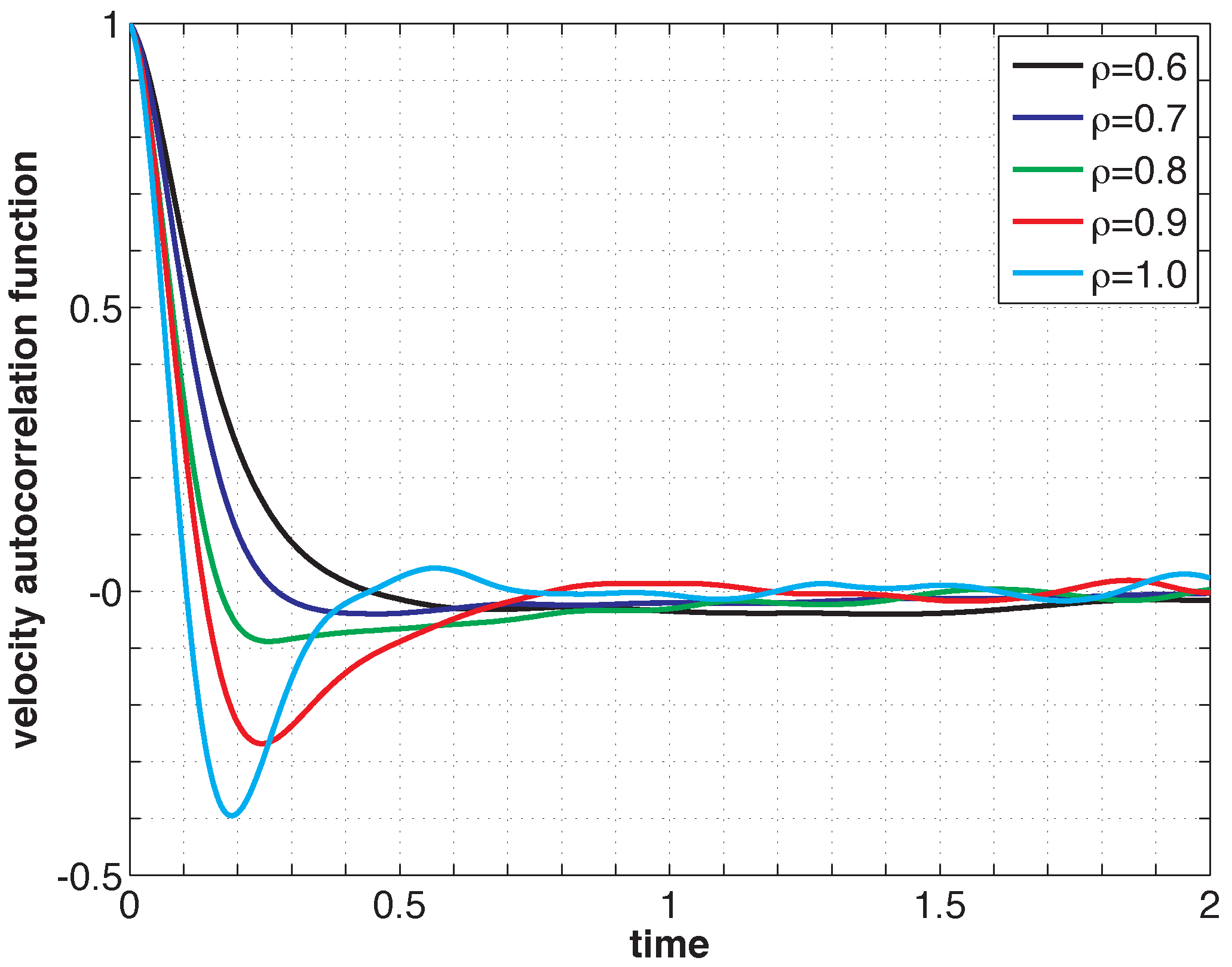
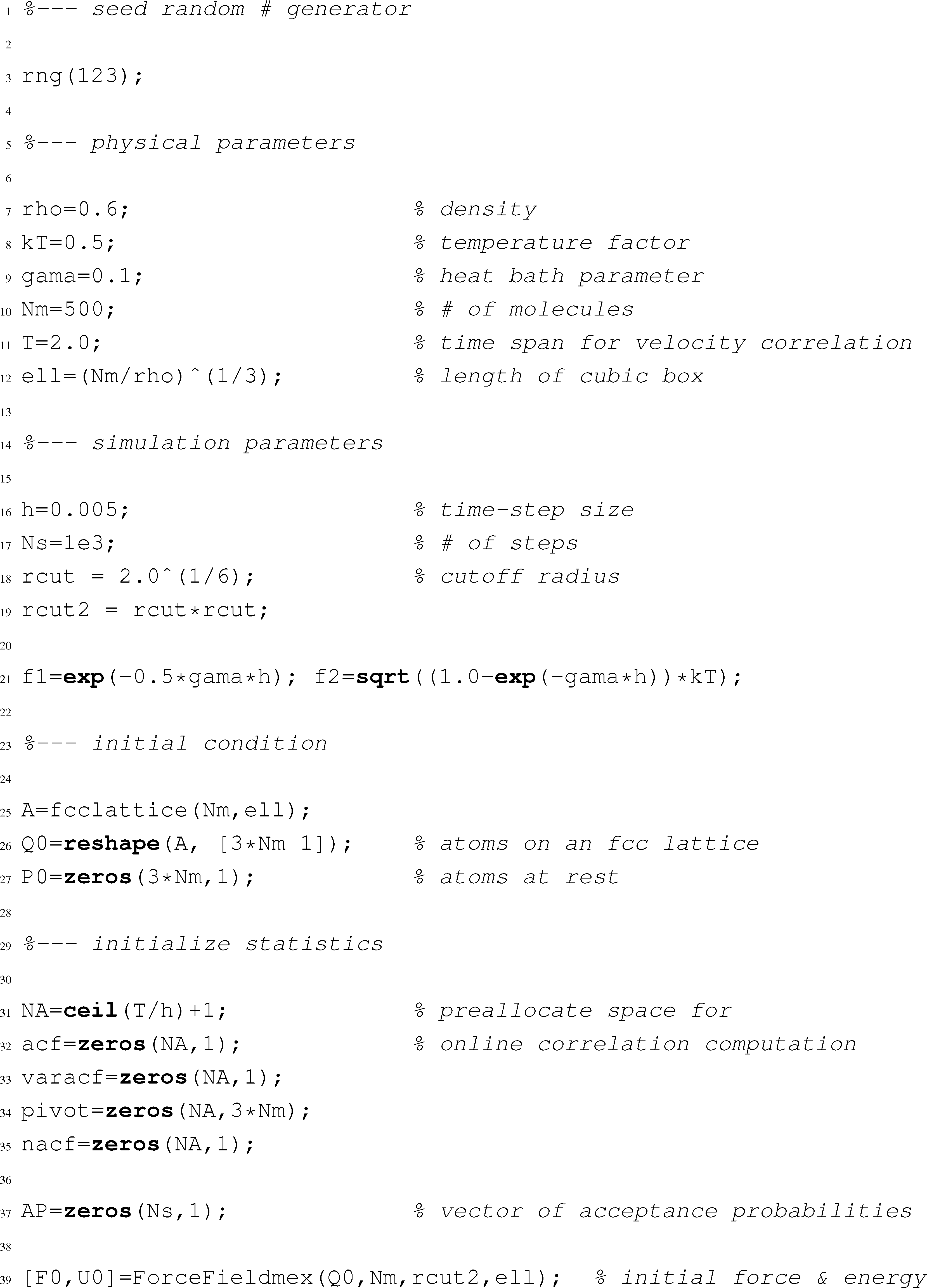
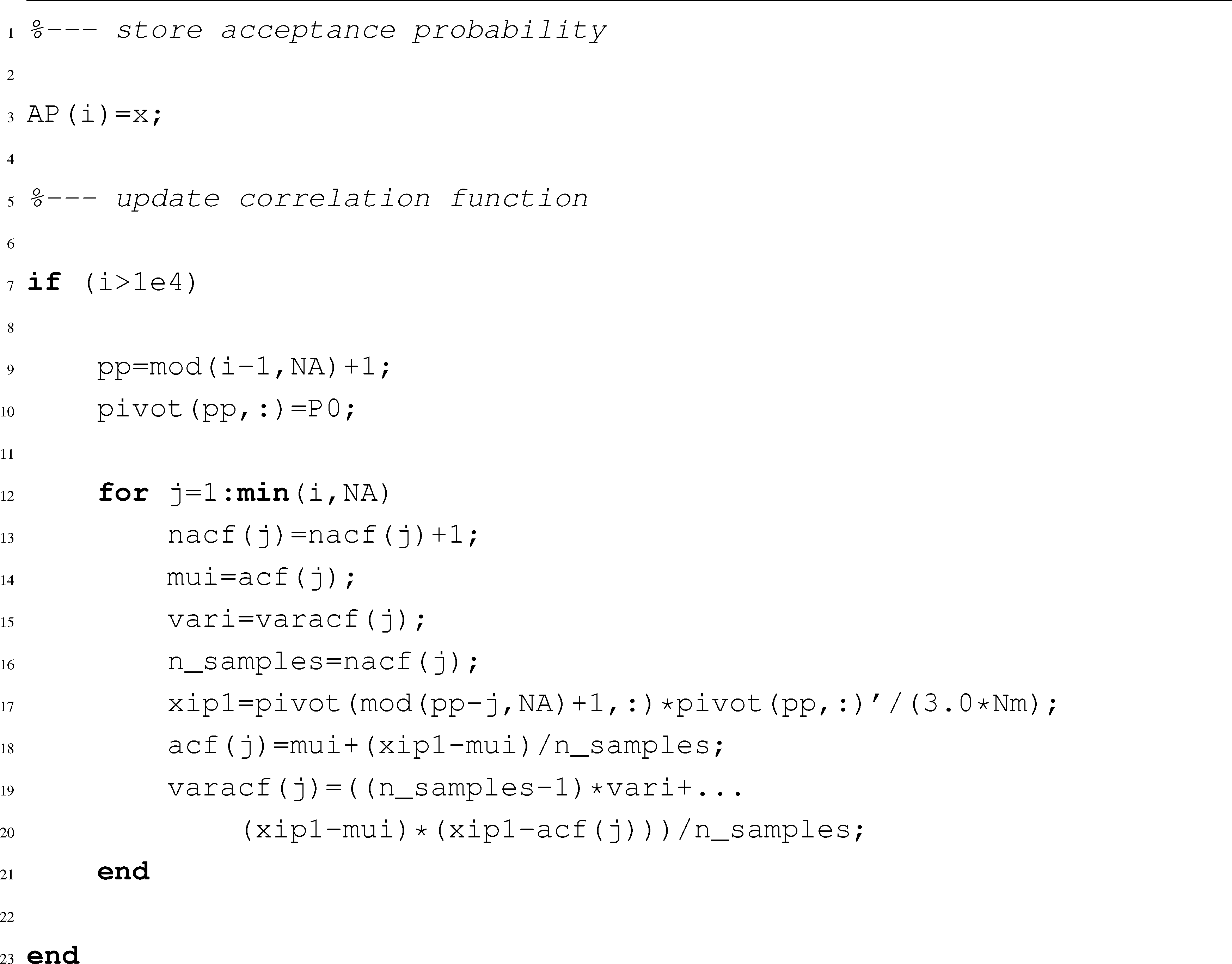
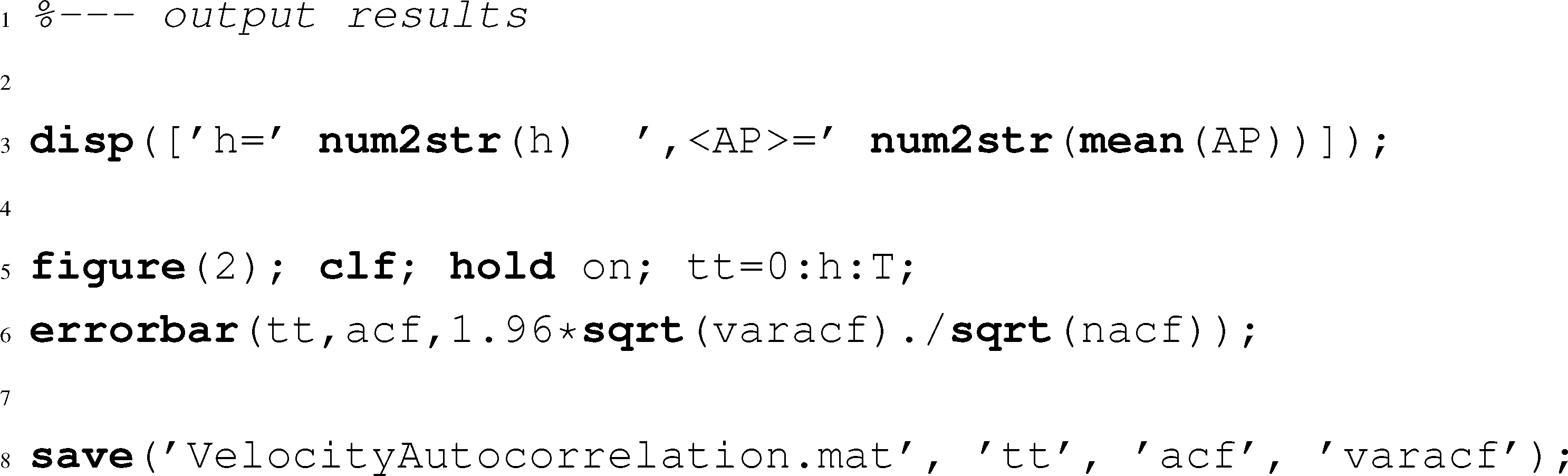
Listing 2 shows the PreProcessing script, which sets the parameters provided in Table 1 and constructs the initial condition, where the N atoms are assumed to be at rest and on the sites of a face-centered cubic lattice. The command, rng(123), on Line 3 sets the seed of the random number generator functions, RAND and RANDN. The acceptance rates at every step and the velocity autocorrelation are updated in the UpdateSampleAverages script shown in Listing 3. The mean acceptance rate, which is outputted in the PostProcessing script shown in Listing 4, must be high enough to ensure that the dynamics is accurately represented. To compute the autocorrelation of an observable over a time interval of length T, the value of that observable along the entire trajectory is not needed. In fact, it suffices to use the values of this observable along a piece of trajectory over a moving time-window [ti, ti + T ], where ti = i × h. This storage space is allocated in PreProcessing and is updated in UpdateSampleAverages. More precisely, the molecular velocities are stored in the pivot array from i − Na to i, where i is the index of the current position and Na = ⌈T/h⌉ + 1. Notice that velocity autocorrelations are not computed until after the index, i, exceeds 104. This equilibration time removes some of the statistical bias that may arise from using a non-random initial condition. Short-time trajectories of this molecular system are plotted in Figure 3 from an initial condition where atoms are placed on the sites of a face-centered cubic lattice and at rest. The trajectory is computed using the numerical and physical parameters indicated in Table 1, with the exception of the number of steps, which is set equal to Ns = 1000. Notice that at lower densities particle trajectories are more diffusive and less localized. Using the parameters provided in Table 1, we compute velocity autocorrelations for a range of density values in Figure 4. Since the heat bath parameter is set to a small value, these figures are in qualitative agreement with those obtained by simulating the molecular system with no heat bath as shown in Figure 5.2 of [3].


5. General Case
Here, we show how the preceding ideas extend to other molecular systems that obey stochastic differential equations. In the process, we generalize the Metropolized Bussi and Parinello integrator (Algorithm 3.2) to a big class of diffusion processes, including the v-rescale thermostat. We begin with the underlying Hamiltonian dynamics of a molecular system.
5.1. Bath-Free Dynamics
MD is based on Hamilton’s equations for a Hamiltonian H: ℝ2d → ℝ:
(S1) volume-preserving (since the vector-field in Equation (11) is divergenceless); and
(S2) energy-preserving (since J is skew-symmetric and constant).
Explicit symplectic integrators, like the Verlet scheme, exploit these properties to obtain long-time stable schemes for Hamilton’s equations [96,97].
5.2. Governing Stochastic Dynamics
In order to mimic experimental conditions, Equation (11) is often coupled to a bath that puts the system at constant temperature and/or pressure. The standard way to do this is to assume that the system with a bath is governed by a stochastic ordinary differential equation (SDE) of the type:

| Y(t) ∈ ℝn | state of the (extended) system |
| A(x) ∈ ℝn | deterministic drift vector field |
| B(x) ∈ ℝn×n | noise-coefficient matrix |
| D(x) ∈ ℝn×n | diffusion matrix |
| W (t) ∈ ℝn | n-dimensional Brownian motion |
| kT | temperature factor |
The n × n diffusion matrix, D(x), is defined in terms of the noise coefficient matrix, B(x), as:
Equation (14) generates a stochastic process, Y (t), that is a Markov diffusion process. We assume that this diffusion process admits a stationary distribution μ(dx), i.e., a probability distribution preserved by the dynamics [98,99]. We denote by ν(x) the density of this distribution. Even though the diffusion matrix in Equation (15) is not necessarily positive definite, one can use the Hörmander’s condition to prove that the process, Y (t), is an ergodic process with a unique stationary distribution [100,101]. By the ergodic theorem, it then follows that:
The evolution of the probability density of the law of Y (t) at time t, ρ(t, x), satisfies the Fokker-Planck equation:
In this case, the operator, L, is self-adjoint, in the sense that:
5.3. Splitting Approach to MD Simulation
We are now in a position to explain our general approach for deriving a long-time stable scheme for Equation (14). Crucial to our approach is that in MD simulation, we usually have a formula for a function proportional to the stationary density ν(x). Following [90], we can split Equation (14) into:
In place of the exact splitting, a Metropolized explicit integrator can be used for Equation (25) [92], and a measure-preserving scheme can be designed to solve the ODE [72,104]. In [92], explicit schemes are introduced for Equation (25) that: (i) sample the exact equilibrium probability density of the SDE when this density exists (i.e., whenever ν(x) is normalizable); (ii) generates a weakly accurate approximation to the solution of Equation (14) at constant kT ; (iii) acquire higher order accuracy in the small noise limit, kT → 0; and (iv) avoid computing the divergence of the diffusion matrix D(x). Compared to the methods in [72], the main novelty of these schemes stems from (iii) and (iv). The resulting explicit splitting method is accurate, since it is an additive splitting of Equation (14); and typically ergodic when the continuous process is ergodic [72].
This type of splitting of Equation (14) is quite natural and has been used before in MD [43,87], dissipative particle dynamics [105,106] and the simulation of inertial particles [107]. Other closely related schemes for Equation (14) include Brünger-Brooks-Karplus (BBK) [35], van Gunsteren and Berendsen (vGB) [108] and the Langevin-Impulse (LI) methods [41] and quasi-symplectic integrators [44]. However, for general MD force fields, none of these explicit integrators are long-time stable. Our framework to stabilize explicit MD integrators is the Metropolis-Hastings algorithm.
5.4. Metropolis-Hastings Algorithm
A Metropolis-Hastings method is a Monte Carlo method for producing samples from a probability distribution, given a formula for a function proportional to its density [74,75]. The algorithm consists of two sub-steps: firstly, a proposal move is generated according to a transition density, g(x, y); and secondly, this proposal move is accepted or rejected with a probability:
6. Conclusions
This paper provided an algorithmic introduction to time integrators for MD simulation. A quick overview of existing algorithms was given. When the derivatives of the potential are bounded, it is well known that these integrators work just fine: they are convergent on finite-time intervals and possess an invariant measure that is nearby the Boltzmann-Gibbs density. However, in realistic MD simulation, the derivatives of the potential are unbounded. This lack of regularity can cause numerical instabilities or artifacts in explicit integrators. The paper demonstrated how a Metropolis acceptance-rejection step can be added to explicit MD integrators to mitigate some of these problems and, in principle, obtain long-time stable and finite-time accurate schemes. A MATLAB implementation of Metropolis-corrected MD integrators was provided and used to compute the velocity autocorrelation of a sea of Lennard-Jones particles at various densities between the solid and liquid phases. The paper did not provide an in-depth review of the theory of Metropolis integrators, which can be found elsewhere [72,73].
Calculating the force field at every step dominates the overall computational cost of MD simulation. These force fields involve: bonded interactions and non-bonded Lennard-Jones and electrostatic interactions. The calculation of bonded interactions is straightforward to vectorize and scales like O(N). In addition, Lennard-Jones forces rapidly decay with interatomic distance. To a good approximation, every atom interacts only with neighbors within a sufficiently large ball. By using data structures, like neighbor lists and cell linked lists, these interactions can be calculated in O(N) steps, and therefore, the Lennard-Jones interactions can be calculated in O(N) steps [46]. On the other hand, the electrostatic energy between particles decays, like 1/r, where r denotes an interatomic distance, which leads to long-range interactions between atoms. Unlike Lennard-Jones interaction, this interaction cannot be cutoff without introducing large errors. In this case, one can use sophisticated techniques, like the fast multipole method, to rigorously handle such interactions in (N) steps [39,58].
However, the effect of these ‘mathematical tricks’ for fast calculation of the force field can become muted if the time step requirement for stability or accuracy becomes more severe in high dimension. This can happen in the Metropolis integrator, if the acceptance probability in Step 2 of Algorithm 3.1 or Step 3 of Algorithm 3.2 deteriorates in high dimension. The scaling of Metropolis algorithms has been quantified for the random walk Metropolis, hybrid Monte Carlo and Metropolis-adjusted Langevin algorithm (MALA) [111–115]. Since the acceptance probability is a function of an extensive quantity, the acceptance rate can artificially deteriorate with increasing system size, unless the time step is reduced. Because high acceptance rates are required to maintain dynamic accuracy, the dependence of the time step on system size limits the application of Metropolized schemes to large-scale systems. Fortunately, this scalability issue can often be resolved by using local, rather than global proposal moves, because the change in energy induced by a local move is typically an intensive quantity. For molecular dynamics calculations, this approach was pursued in [73]. Using dynamically consistent local moves (a so-called J-splitting [116]), it was shown that in certain situations, a scalable Metropolis integrator can be designed; however, the extent to which this strategy remedies the issue of high rejection rate in high dimension is not clear at this point and should be tested in applications.
Acknowledgments
The author wishes to acknowledge Eric Vanden-Eijnden for useful comments on an earlier version of this paper. The research that led to this paper was funded by the US National Science Foundation through Division of Mathematical Sciences (DMS) grant # DMS-1212058.
Conflicts of Interest
The authors declare no conflict of interest.
References
- Allen, M.P.; Tildesley, D.J. Computer Simulation of Liquids; Clarendon Press: Oxford, UK, 1987. [Google Scholar]
- Frenkel, D.; Smit, B. Understanding Molecular Simulation: From Algorithms to Applications, 2nd ed.; Academic Press: Waltham, MA, USA, 2002. [Google Scholar]
- Rapaport, D.C. The Art of Molecular Dynamics Simulation; Cambridge University Press: Cambridge, UK, 2004. [Google Scholar]
- Tuckerman, M. Statistical Mechanics and Molecular Simulations; Oxford University Press: Oxford, UK, 2008. [Google Scholar]
- Schlick, T. Molecular Modeling and Simulation: An Interdisciplinary Guide; Springer: Berlin/Heidelberg, Germany, 2010; Volume 21, . [Google Scholar]
- Rahman, A. Correlations in the motion of atoms in liquid argon. Phys. Rev 1964, 136, A405. [Google Scholar]
- Verlet, L. Computer “experiments” on classical fluids. I. Thermodynamical properties of Lennard-Jones molecules. Phys. Rev 1967, 159, 98–103. [Google Scholar]
- Alder, B.J.; Wainwright, T.E. Velocity autocorrelations for hard spheres. Phys. Rev. Lett 1967, 18, 988–990. [Google Scholar]
- Alder, B.J.; Gass, D.M.; Wainwright, T.E. Studies in molecular dynamics. VIII. The transport coefficients for a hard-sphere fluid. J. Chem. Phys 1970, 53, 3813–3826. [Google Scholar]
- Harp, G.D.; Berne, B.J. Time-correlation functions, memory functions, and molecular dynamics. Phys. Rev. A 1970, 2, 975–996. [Google Scholar]
- Rahman, A.; Stillinger, F.H. Molecular dynamics study of liquid water. J. Chem. Phys 1971, 55, 3336–3359. [Google Scholar]
- Stillinger, F.H.; Rahman, A. Improved simulation of liquid water by molecular dynamics. J. Chem. Phys 1974, 60, 1545–1557. [Google Scholar]
- Stillinger, F.H. Water revisited. Science 1980, 209, 451–457. [Google Scholar]
- McCammon, A.J.; Gelin, B.R.; Karplus, M. Dynamics of folded proteins. Nature 1977, 267, 585–590. [Google Scholar]
- Van Gunsteren, W.F.; Berendsen, H.J.C. Algorithms for macromolecular dynamics and constraint dynamics. Mol. Phys 1977, 34, 1311–1327. [Google Scholar]
- McCammon, J.A.; Karplus, M. Simulation of protein dynamics. Annu. Rev. Phys. Chem 1980, 31, 29–45. [Google Scholar]
- Van Gunsteren, W.F.; Karplus, M. Protein dynamics in solution and in a crystalline environment: A molecular dynamics study. Biochemistry 1982, 21, 2259–2274. [Google Scholar]
- Karplus, M.; McCammon, A.J. Dynamics of proteins: Elements and function. Annu. Rev. Biochem 1983, 52, 263–300. [Google Scholar]
- Van Gunsteren, W.F.; Berendsen, H.J.C. Computer simulation of molecular dynamics: Methodology, applications, and perspectives in chemistry. Angew. Chem. Int. Ed. Engl 1990, 29, 992–1023. [Google Scholar]
- Karplus, M.; McCammon, A.J. Molecular dynamics simulations of biomolecules. Nat. Struct. Mol. Biol 2002, 9, 646–652. [Google Scholar]
- Case, D.A. Molecular dynamics and NMR spin relaxation in proteins. Acc. Chem. Res 2002, 35, 325–331. [Google Scholar]
- Adcock, A.S.; McCammon, A.J. Molecular dynamics: Survey of methods for simulating the activity of proteins. Chem. Rev 2006, 106, 1589–1615. [Google Scholar]
- Van Gunsteren, W.F.; Dolenc, J.; Mark, A.E. Molecular simulation as an aid to experimentalists. Curr. Opin. Struct. Biol 2008, 18, 149–153. [Google Scholar]
- Kapral, R.; Ciccotti, G. Molecular dynamics: An Account of its Evolution. In Theory and Applications of Computational Chemistry: The First Forty Years; Elsevier: New York, NY, USA, 2005; pp. 425–441. [Google Scholar]
- Levitt, M. Molecular dynamics of native protein: I. Computer simulation of trajectories. J. Mol. Biol 1983, 168, 595–617. [Google Scholar]
- Levitt, M.; Sharon, R. Accurate simulation of protein dynamics in solution. Proc. Natl. Acad. Sci. USA 1988, 85, 7557–7561. [Google Scholar]
- Daggett, V.; Levitt, M. A model of the molten globule state from molecular dynamics simulations. Proc. Natl. Acad. Sci. USA 1992, 89, 5142–5146. [Google Scholar]
- Li, A.; Daggett, V. Investigation of the solution structure of chymotrypsin inhibitor 2 using molecular dynamics: Comparison to X-Ray crystallographic and NMR data. Protein Eng 1995, 8, 1117–1128. [Google Scholar]
- Duan, Y.; Kollman, P.A. Pathways to a protein folding intermediate observed in a 1-microsecond simulation in aqueous solution. Science 1998, 282, 740–744. [Google Scholar]
- Freddolino, P.L.; Liu, F.; Gruebele, M.; Schulten, K. Ten-microsecond molecular dynamics simulation of a fast-folding WW domain. Biophys. J 2008, 94, 75–77. [Google Scholar]
- Shaw, D.E.; Maragakis, P.; Lindorff-Larsen, K.; Piana, S.; Dror, R.O.; Eastwood, M.P.; Bank, J.A.; Jumper, J.M.; Salmon, J.K.; Shan, Y. Atomic-level characterization of the structural dynamics of proteins. Science 2010, 330, 341–346. [Google Scholar]
- Quentrec, B.; Brot, C. New method for searching for neighbors in molecular dynamics computations. J. Comput. Phys 1973, 13, 430–432. [Google Scholar]
- Ryckaert, J.P.; Ciccotti, G.; Berendsen, H.J.C. Numerical integration of the Cartesian equations of motion of a system with constraints: Molecular dynamics of n-Alkanes. J. Comput. Phys 1977, 23, 327–341. [Google Scholar]
- Schneider, T.; Stoll, E. Molecular dynamics study of a three-dimensional one-component model for distortive phase transitions. Phys. Rev. B 1978, 17, 1302–1322. [Google Scholar]
- Brünger, A.; Brooks, C.L.; Karplus, M. Stochastic boundary conditions for molecular dynamics simulations of ST2 water. Chem. Phys. Lett 1984, 105, 495–500. [Google Scholar]
- Brooks, B.R.; Bruccoleri, R.E.; Olafson, B.D.; States, D.J.; Swaminathan, S.; Karplus, M. CHARMM: A program for macromolecular energy, minimization, and dynamics calculations. J. Comput. Chem 1983, 4, 187–217. [Google Scholar]
- Nosé, S. A unified formulation for constant temperature molecular dynamics methods. J. Chem. Phys 1984, 81, 511–519. [Google Scholar]
- Hoover, W.G. Canonical dynamics: Equilibrium phase-space distributions. Phys. Rev. A 1985, 31, 1695–1697. [Google Scholar]
- Greengard, L.; Rokhlin, V. A fast algorithm for particle simulations. J. Comput. Phys 1987, 73, 325–348. [Google Scholar]
- Tuckerman, M.E.; Berne, B.J.; Martyna, G. Reversible multiple time scale molecular dynamics. J. Chem. Phys 1992, 97, 1990–2001. [Google Scholar]
- Skeel, R.D.; Izaguirre, J. An impulse integrator for Langevin dynamics. Mol. Phys 2002, 100, 3885–3891. [Google Scholar]
- Ricci, A.; Ciccotti, G. Algorithms for Brownian dynamics. Mol. Phys 2003, 101, 1927–1931. [Google Scholar]
- Bussi, G.; Parrinello, M. Accurate sampling using Langevin dynamics. Phys. Rev. E 2007, 75, 056707. [Google Scholar]
- Milstein, G.N.; Tretyakov, M.V. Quasi-symplectic methods for Langevin-type equations. IMA J. Num. Anal 2003, 23, 593–626. [Google Scholar]
- Milstein, G.N.; Tretyakov, M.V. Computing ergodic limits for Langevin equations. Physica D 2007, 229, 81–95. [Google Scholar]
- Yao, Z.; Wang, J.S.; Liu, G.R.; Cheng, M. Improved neighbor list algorithm in molecular simulations using cell decomposition and data sorting method. Comput. Phys. Commun 2004, 161, 27–35. [Google Scholar]
- Bussi, G.; Donadio, D.; Parrinello, M. Canonical sampling through velocity rescaling. J. Chem. Phys 2007, 126, 014101. [Google Scholar]
- Samoletov, A.A.; Chaplain, M.A.; Dettmann, C.P. Thermostats for “Slow” configurational modes. J. Stat. Phys 2008, 128, 1321–1336. [Google Scholar]
- Leimkuhler, B.; Noorizadeh, E.; Theil, F. A gentle stochastic thermostat for molecular dynamics. J. Stat. Phys 2009, 135, 261–277. [Google Scholar]
- Leimkuhler, B.; Reich, S. A. Metropolis adjusted Nosé-Hoover thermostat. Math. Model. Num. Anal 2009, 43, 743–755. [Google Scholar]
- Scheraga, H.A.; Khalili, M.; Liwo, A. Protein-folding dynamics: Overview of molecular simulation techniques. Annu. Rev. Phys. Chem 2007, 58, 57–83. [Google Scholar]
- Dror, R.O.; Dirks, R.M.; Grossman, J.P.; Xu, H.; Shaw, D.E. Biomolecular simulation: A computational microscope for molecular biology. Annu. Rev. Biophys 2012, 41, 429–452. [Google Scholar]
- Lane, T.J.; Shukla, D.; Beauchamp, K.A.; Pande, V.S. To milliseconds and beyond: Challenges in the simulation of protein folding. Curr. Opin. Struct. Biol 2013, 23, 58–65. [Google Scholar]
- Nielsen, S.O.; Lopez, C.F.; Srinivas, G.; Klein, M.L. Coarse grain models and the computer simulation of soft materials. J. Phys. Condens. Matter 2004, 16, R481. [Google Scholar]
- Tozzini, V. Coarse-grained models for proteins. Curr. Opin. Struct. Biol 2005, 15, 144–150. [Google Scholar]
- Clementi, C. Coarse-grained models of protein folding: Toy models or predictive tools? Curr. Opin. Struct. Biol 2008, 18, 10–15. [Google Scholar]
- Sherwood, P.; Brooks, B.R.; Sansom, M.S.P. Multiscale methods for macromolecular simulations. Curr. Opin. Struct. Biol 2008, 18, 630–640. [Google Scholar]
- Weinan, E. Principles of Multiscale Modeling; Cambridge University Press: Cambridge, UK, 2011. [Google Scholar]
- Weinan, E.; Vanden-Eijnden, E. Metastability Conformation Dynamics, and TransitionPathwaysin Complex Systems. Attinger, S., Koumoutsakos, P., Eds.; Springer: Berlin/Heidelberg, Germany, 2004; pp. 35–68. [Google Scholar]
- Vanden-Eijnden, E.; Venturoli, M. Markovian milestoning with Voronoi tessellations. J. Chem. Phys 2009, 130, 194101. [Google Scholar]
- Vanden-Eijnden, E.; Venturoli, M. Exact rate calculations by trajectory parallelization and twisting. J. Chem. Phys 2009, 131, 044120. [Google Scholar]
- Weinan, E.; Vanden-Eijnden, E. Transition-path theory and path-finding algorithms for the study of rare events. Annu. Rev. Phys. Chem 2010, 61, 391–420. [Google Scholar]
- Nelson, M.T.; Humphrey, W.; Gursoy, A.; Dalke, A.; Kalé, L.V.; Skeel, R.D.; Schulten, K. NAMD: A parallel, object-oriented molecular dynamics program. Int. J. High Perform. Comput. Appl 1996, 10, 251–268. [Google Scholar]
- Scott, W.R.P.; Hünenberger, P.H.; Tironi, I.G.; Mark, A.E.; Billeter, S.R.; Fennen, J.; Torda, A.E.; Huber, T.; Krüger, P.; van Gunsteren, W.F. The GROMOS biomolecular simulation program package. J. Phys. Chem. A 1999, 103, 3596–3607. [Google Scholar]
- Talay, D. Stochastic Hamiltonian systems: Exponential convergence to the invariant measure, and discretization by the implicit Euler scheme. Markov Process. Relat. Fields 2002, 8, 1–36. [Google Scholar]
- Higham, D.J.; Mao, X.; Stuart, A.M. Strong convergence of Euler-type methods for nonlinear stochastic differential equations. IMA J. Num. Anal 2002, 40, 1041–1063. [Google Scholar]
- Milstein, G.N.; Tretyakov, M.V. Numerical integration of stochastic differential equations with nonglobally Lipschitz coefficients. IMA J. Num. Anal 2005, 43, 1139–1154. [Google Scholar]
- Higham, D.J. Stochastic ordinary differential equations in applied and computational mathematics. IMA J. Appl. Math 2011, 76, 449–474. [Google Scholar]
- Hutzenthaler, M.; Jentzen, A.; Kloeden, P.E. Strong convergence of an explicit numerical method for SDEs with non-globally Lipschitz continuous coefficients. Ann. Appl. Probab 2012, 22, 1611–1641. [Google Scholar]
- Scemama, A.; Lelièvre, T.; Stoltz, G.; Cancés, E.; Caffarel, M. An efficient sampling algorithm for variational Monte Carlo. J. Chem. Phys 2006, 125, 114105. [Google Scholar]
- Akhmatskaya, E.; Bou-Rabee, N.; Reich, S. A comparison of generalized hybrid Monte Carlo methods with and without momentum flip. J. Comput. Phys 2009, 228, 2256–2265. [Google Scholar]
- Bou-Rabee, N.; Vanden-Eijnden, E. Pathwise accuracy and ergodicity of Metropolized integrators for SDEs. Commun. Pure Appl. Math 2010, 63, 655–696. [Google Scholar]
- Bou-Rabee, N.; Vanden-Eijnden, E. A patch that imparts unconditional stability to explicit integrators for Langevin-like equations. J. Comput. Phys 2012, 231, 2565–2580. [Google Scholar]
- Metropolis, N.; Rosenbluth, A.W.; Rosenbluth, M.N.; Teller, A.H.; Teller, E. Equations of state calculations by fast computing machines. J. Chem. Phys 1953, 21, 1087–1092. [Google Scholar]
- Hastings, W.K. Monte-Carlo methods using Markov chains and their applications. Biometrika 1970, 57, 97–109. [Google Scholar]
- Rossky, P.J.; Doll, J.D.; Friedman, H.L. Brownian dynamics as smart Monte Carlo simulation. J. Chem. Phys 1978, 69, 4628. [Google Scholar]
- Duane, S.; Kennedy, A.D.; Pendleton, B.J.; Roweth, D. Hybrid Monte-Carlo. Phys. Lett. B 1987, 195, 216–222. [Google Scholar]
- Horowitz, A.M. A generalized guided Monte-Carlo algorithm. Phys. Lett. B 1991, 268, 247–252. [Google Scholar]
- Kennedy, A.D.; Pendleton, B. Cost of the generalized hybrid Monte Carlo algorithm for free field theory. Nucl. Phys. B 2001, 607, 456–510. [Google Scholar]
- Liu, J.S. Monte Carlo Strategies in Scientific Computing, 2nd ed.; Springer: Berlin/Heidelberg, Germany, 2008. [Google Scholar]
- Akhmatskaya, E.; Reich, S. GSHMC: An efficient method for molecular simulation. J. Comput. Phys 2008, 227, 4937–4954. [Google Scholar]
- Lelièvre, T.; Rousset, M.; Stoltz, G. Free Energy Computations: A Mathematical Perspective, 1st ed.; Imperial College Press: London, UK, 2010. [Google Scholar]
- MATLAB, Version 8.0.0 (R2012b); The MathWorks Inc: Natick, MA, USA, 2012.
- Introducing MEX-Files. Available online: http://www.mathworks.com/help/matlab/matlab_external/introducing-mex-files.html (accessed on 19 September 2013).
- Kloeden, P.E.; Platen, E. Numerical Solution of Stochastic Differential Equations; Springer: Berlin, Germany, 1992. [Google Scholar]
- Hutzenthaler, M.; Jentzen, A.; Kloeden, P.E. Strong and weak divergence in finite time of Euler’s method for stochastic differential equations with non-globally Lipschitz continuous coefficients. Proc. R. Soc. A: Math. Phys. Eng. Sci 2011, 467, 1563–1576. [Google Scholar]
- Vanden-Eijnden, E.; Ciccotti, G. Second-order integrators for Langevin equations with holonomic constraints. Chem. Phys. Lett 2006, 429, 310–316. [Google Scholar]
- Leimkuhler, B.; Matthews, C. Robust and efficient configurational molecular sampling via Langevin dynamics. J. Chem. Phys 2013, 138, 174102. [Google Scholar]
- Evans, L. An Introduction to Stochastic Differential Equations; American Mathematical Society: Providence, RI, USA, 2013. [Google Scholar]
- Bou-Rabee, N.; Owhadi, H. Long-run accuracy of variational integrators in the stochastic context. SIAM J. Numer. Anal 2010, 48, 278–297. [Google Scholar]
- Leimkuhler, B.; Matthews, C.; Stoltz, G. The computation of averages from equilibrium and nonequilibrium Langevin molecular dynamics. 2013. arXiv:1308.5814. [Google Scholar]
- Bou-Rabee, N.; Donev, A.; Vanden-Eijnden, E. Metropolized integration schemes for self-adjoint diffusions. 2013. arXiv:1309.5037. [Google Scholar]
- Milstein, G.N.; Tretyakov, M.V. Stochastic Numerics for Mathematical Physics; Springer: Berlin, Germany, 2004. [Google Scholar]
- Marsden, J.E; Ratiu, T.S. Introduction to Mechanics and Symmetry: A Basic Exposition of Classical Mechanical Systems; Springer: Berlin/Heidelberg, Germany, 1999. [Google Scholar]
- Van Gunsteren, W.F.; Mark, A.E. Validation of molecular dynamics simulation. J. Chem. Phys 1998, 108, 6109–6116. [Google Scholar]
- Leimkuhler, B.; Reich, S. Simulating Hamiltonian Dynamics; Cambridge Monographs on Applied and Computational Mathematics; Cambridge University Press: Cambridge, UK, 2004. [Google Scholar]
- Hairer, E.; Lubich, C.; Wanner, G. Geometric Numerical Integration; Springer: Berlin/Heidelberg, Germany, 2010. [Google Scholar]
- Ikeda, N.; Watanabe, S. Stochastic Differential Equations and Diffusion Processes; North-Holland: Amsterdam, The Netherlands, 1989. [Google Scholar]
- Klebaner, F.C. Introduction to Stochastic Calculus with Applications; Imperial College Press: London, UK, 2005. [Google Scholar]
- Mengersen, K.L.; Tweedie, R.L. Rates of convergence of the Hastings and Metropolis algorithms. Ann. Stat 1996, 24, 101–121. [Google Scholar]
- Prato, G.D.; Zabczyk, J. Ergodicity for Infinite Dimensional Systems; Cambridge University Press: Cambridge, UK, 1996. [Google Scholar]
- Haussman, U.G.; Pardoux, E. Time reversal for diffusions. Ann. Probab 1986, 14, 1188–1205. [Google Scholar]
- Kent, J. Time-reversible diffusions. Adv. Appl. Prob 1978, 10, 819–835. [Google Scholar]
- Ezra, G.S. Reversible measure-preserving integrators for non-Hamiltonian systems. J. Chem. Phys 2006, 125, 034104. [Google Scholar]
- Shardlow, T. Splitting for dissipative particle dynamics. SIAM J. Sci. Comput 2003, 24, 1267–1282. [Google Scholar]
- Serrano, M.; de Fabritiis, G.; Espanol, P.; Coveney, P.V. A stochastic Trotter integration scheme for dissipative particle dynamics. Math. Comput. Simulat 2006, 72, 190–194. [Google Scholar]
- Pavliotis, G.A.; Stuart, A.M.; Zygalakis, K.C. Calculating effective diffusivities in the limit of vanishing molecular diffusion. J. Comput. Phys 2008, 228, 1030–1055. [Google Scholar]
- Van Gunsteren, W.F.; Berendsen, H.J.C. Algorithms for Brownian dynamics. Mol. Phys 1982, 45, 637–647. [Google Scholar]
- Nummelin, E. General Irreducible Markov Chains and Non-Negative Operators; Cambridge University Press: New York, NY, USA, 1984. [Google Scholar]
- Tierney, L. Markov chains for exploring posterior distributions. Ann. Stat 1994, 22, 1701–1728. [Google Scholar]
- Gelman, A.; Gilks, W.R.; Roberts, G.O. Weak convergence and optimal scaling of random walk Metropolis algorithms. Ann. Appl. Probab 1997, 7, 110–120. [Google Scholar]
- Roberts, G.O.; Rosenthal, J.S. Optimal scaling of discrete approximations to Langevin diffusions. J. R. Stat. Soc. Ser. B 1998, 60, 255–268. [Google Scholar]
- Beskos, A.; Roberts, G.O.; Stuart, A.M. Optimal scalings for local Metropolis-Hastings chains on non-product targets in high dimensions. Ann. Appl. Probab 2009, 19, 863–898. [Google Scholar]
- Beskos, A.; Pillai, N.S.; Roberts, G.O.; Sanz-Serna, J.M.; Stuart, A.M. Optimal tuning of hybrid Monte-Carlo algorithm. 2010. arXiv:1001.4460.
- Mattingly, J.C.; Pillai, N.S.; Stuart, A.M. Diffusion limits of the random walk Metropolis algorithm in high dimensions. Ann. Appl. Probab 2012, 22, 881–930. [Google Scholar]
- Kang, F.; Dao-Liu, W. Dynamical Systems and Geometric Construction of Algorithms. In Computational Mathematics in China; Contemporary Mathmatics, Volume 163; Shi, Z.-C., Yang, C.C., Eds.; American Mathmatical Society: New York, NY, USA, 1994; pp. 1–32. [Google Scholar]


| Parameter | Description | Value | |
|---|---|---|---|
| Physical Parameters | ρ | density | {0.6, 0.7, 0.8, 0.9, 1.0, 1.1} |
| kT | temperature factor | 0.5 | |
| γ | heat bath parameter | 0.01 | |
| Nm | # of molecules | 512 | |
| T | time-span for autocorrelation | 2 | |
| Numerical Parameters | h | time step | 0.005 |
| Ns | # of simulation steps | 105 | |
| rc | Lennard-Jones force cutoff radius | 21/6 | |
© 2014 by the authors; licensee MDPI, Basel, Switzerland This article is an open access article distributed under the terms and conditions of the Creative Commons Attribution license (http://creativecommons.org/licenses/by/3.0/).
Share and Cite
Bou-Rabee, N. Time Integrators for Molecular Dynamics. Entropy 2014, 16, 138-162. https://0-doi-org.brum.beds.ac.uk/10.3390/e16010138
Bou-Rabee N. Time Integrators for Molecular Dynamics. Entropy. 2014; 16(1):138-162. https://0-doi-org.brum.beds.ac.uk/10.3390/e16010138
Chicago/Turabian StyleBou-Rabee, Nawaf. 2014. "Time Integrators for Molecular Dynamics" Entropy 16, no. 1: 138-162. https://0-doi-org.brum.beds.ac.uk/10.3390/e16010138