Correlation Functions in Open Quantum-Classical Systems

Abstract
: Quantum time correlation functions are often the principal objects of interest in experimental investigations of the dynamics of quantum systems. For instance, transport properties, such as diffusion and reaction rate coefficients, can be obtained by integrating these functions. The evaluation of such correlation functions entails sampling from quantum equilibrium density operators and quantum time evolution of operators. For condensed phase and complex systems, where quantum dynamics is difficult to carry out, approximations must often be made to compute these functions. We present a general scheme for the computation of correlation functions, which preserves the full quantum equilibrium structure of the system and approximates the time evolution with quantum-classical Liouville dynamics. Several aspects of the scheme are discussed, including a practical and general approach to sample the quantum equilibrium density, the properties of the quantum-classical Liouville equation in the context of correlation function computations, simulation schemes for the approximate dynamics and their interpretation and connections to other approximate quantum dynamical methods.1. Introduction
The dynamical properties of condensed-phase or complex systems are often investigated experimentally by applying external fields to weakly perturb a system and observe its relaxation back to the thermal equilibrium state. In such experiments, measurable quantities can be related to equilibrium time correlation functions via linear response theory [1,2]:
Exact numerical evaluation of Equation (1) for real condensed phase quantum systems is prohibitive, since the computational cost scales exponentially with respect to the number of degrees of freedom (DOF). Various approaches have been developed to address this challenging problem. A common approach shared by many methods is to partition the entire system into a subsystem (whose dynamical properties are of interest) and an environment (or bath) in which the subsystem resides. Other recently developed schemes for computing quantum correlation functions do not rely on such a partition and instead utilize approximations to treat the quantum evolution of the entire system in conjunction with quantum equilibrium sampling [3–5]. In this paper, we focus on schemes based on the system-bath partition, and using this partition, the Hamiltonian reads: Ĥ= Ĥb+ĥs+V̂c(R̂); where and ĥs represent the pure bath and subsystem Hamiltonians, respectively. The last term in Ĥ is a coupling potential that depends on the spatial coordinates of the bath wave functions. We shall always take the bath part of the Hamiltonian in the coordinate representation; however, we can represent in some quantum basis: .
Several methods based on various master equations [6–10] and path integral influence functional methods [11,12] provide approximate schemes, often in the weak coupling limit, to systematically project out the environmental DOF and yield a subsystem dynamics that incorporates dissipation and decoherence, due to coupling to the environment. However, for many applications, such as proton and electron transfer in condensed phases, it is desirable to explicitly simulate, even approximately, the bath dynamics, since specific local bath DOF may be crucial for a description of the dynamics of the quantum subsystem. For this purpose, several semiclassical [13–15] and mixed quantum-classical [16,17] (MQC) methods, which either treat the entire dynamics semiclassically or simulate the dynamics of the bath and subsystem with different levels of rigor (e.g., classical versus quantum mechanical), have been formulated. Many semiclassical and mixed quantum-classical approaches, adopting powerful classical simulation techniques, evaluate Equation (1) by combined Monte Carlo-molecular dynamics (MC-MD) techniques.
In this paper, we formulate MC-MD schemes to evaluate Equation (1) within the framework of the quantum-classical Liouville equation (QCLE) [18]. The QCLE employs a partial Wigner representation of the environmental (bath) DOF and may be derived from full quantum dynamics by truncating the quantum evolution operator to the first order in a small parameter related to the ratio of the characteristic masses of quantum and bath DOF [18]. In particular, we suppose that the quantum subsystem has a finite-dimension Hilbert space. Under this assumption, Equation (1) is cast in the following form [19,20]:
Two main tasks are involved in evaluating Equation (2) with an MC-MD algorithm. First, one needs to sample initial conditions (for an ensemble of trajectories) from the partially Wigner-transformed quantum density, with ρeq = e−βĤ/ZQ. There exist numerical algorithms to accomplish such a task [21,22]. Second, one needs to propagate the initial points in the phase space. These time-evolved trajectories may then be used to construct the matrix elements, , needed to compute the correlation function. Various simulation methods, whose structure depends on the basis chosen to represent the quantum degrees of freedom in the QCLE, have been devised to simulate the mixed quantum-classical dynamics [23–31]. Simulation methods that utilize an adiabatic basis can be cast into the form of surface-hopping dynamics, but in a way that includes coherent evolution segments that account for creation and destruction of coherence in a proper manner. More recently, as in some semiclassical approaches [32], the mapping basis [33] was used to describe the quantum degrees of freedom in the QCLE in a continuous classical-like manner, leading to a trajectory description in the full system phase space [30,31,34–36].
The goals and outline of the paper are as follows: We first consider how the two ingredients, quantum equilibrium sampling and evolution of quantum operators, which are needed to compute quantum correlation functions, may be carried out. In Section 2, we describe a path-integral scheme to perform MC sampling from the partially Wigner transformed quantum density. In the Appendix, we also discuss a simplified, but approximate sampling scheme that is useful in the high-temperature limit. Another aim of this paper is to demonstrate how a recently-developed simulation method for the QCLE, the forward-backward trajectory solution (FBTS), can be used to efficiently obtain quantum correlation functions. To place these results in proper context, in Section 3, we sketch the important features and properties of the QCLE and discuss both the adiabatic Trotter-based surface-hopping (TBSH) algorithm and the FBTS, which is formulated in the mapping basis. In this section, we also present the explicit form of the N-level generalization of the TBSH algorithm. Comparisons of the trajectories that underlie these algorithms allow us to investigate how completely different ensembles of trajectories can be used to simulate the same observable correlation function. The implementation and utility of the simulation algorithms are illustrated on the dynamics in a two-level system coupled to a quartic oscillator embedded in a bath of independent harmonic oscillators, described in Section 4. Finally, in Section 5, we comment on the advantages, challenges and potential problems in adopting an approximate mixed quantum-classical dynamics for the computation of quantum time-correlation functions.
2. Sampling from the Partially Wigner-Transformed Density
In general, analytical expressions for the Wigner transform of the density matrix cannot be determined easily. In this section, we present a path-integral-based scheme to perform MC sampling from the Wigner-transformed density, , in Equation (2).
First, we recall the definition of partial Wigner transform:
3. Quantum-Classical Liouville Equation
In this section, we discuss how one can simulate the time-evolved matrix elements, , in Equation (2) using the QCLE:
The QCLE has many desirable features, such as the conservation of energy, momentum and phase space volumes. Furthermore, the QCLE is equivalent to full quantum dynamics for arbitrary quantum subsystems, which are bilinearly coupled to a harmonic bath. For instance, commonly used spin boson models are of this type. In this circumstance, the combination of quantum and classical brackets in the QCLE does have a Lie algebraic structure. For the more general bath and coupling potentials, the QCLE provides an approximate description of the quantum dynamics. In this case, comparisons of simulations of QCL dynamics with exact quantum results have indicated that it is quantitatively accurate for a wide range of systems [36,39–48]
The QCLE equation can be simulated using ensembles of trajectories, which, in combination with the quantum initial condition sampling discussed above, provides a way to compute quantum correlation functions. As we shall see, the nature of the trajectories that enter in the simulations depends on the algorithm and should not be ascribed physical significance. It is only the observable, in this case, the correlation function, that has physical meaning and is independent of the manner in which it is simulated, provided the simulation algorithm is capable of exactly solving the QCLE, which is not always the case. One of the goals of this paper is to illustrate how a recently-developed FBTS [31] can be used to easily compute quantum correlation functions. For this purpose, it is interesting to contrast the solution using this scheme, and the trajectory description that underlies it, with the previously-developed and frequently-used TBSH algorithm [26]. Taking the adiabatic representation of the QCL superoperator is the key step in implementing the TBSH algorithm. The last representation of QCLE in Equation (8) resembles the quantum Liouville equation and forms the starting point of the FBTS.
3.1. Adiabatic Trotter-Based Surface Hopping
In order to discuss the nature of the trajectory description involved in the TBSH algorithm, we briefly describe how it is implemented and, in particular, present the explicit generalization to an N-level quantum subsystem, which was only outlined in [26]. We first consider the adiabatic representation of the QCLE, since the TBSH algorithm is cast in this basis. The adiabatic basis is defined by ĥW(R) | α; R〉 = Eα(R) | α; R〉, where ĥW(R) = ĤW(R) − P2/2M is taken to be the adiabatic Hamiltonian for a static configuration of R in this section. In the adiabatic basis, the QCLE reads:
Equation (10) admits a formal solution:
At this point, we have specified all the necessary details in order to simulate the QCL dynamics in the adiabatic basis:
In this algorithm, we see that the trajectories in the ensemble that are used to simulate the time evolution are non-Newtonian in character, consisting of Newtonian segments where the system evolves on adiabatic surfaces, or the mean of two adiabatic surfaces, interspersed with quantum transitions and momentum changes.
3.2. Forward-Backward Trajectory Solution
This scheme is motivated by another way of writing the formally exact solution [38] of the QCLE using the last line of Equation (8):
One approach to solve Equation (25) is to apply the mapping transformation in which N discrete quantum states of the subsystem are represented by the continuous position and momenta of N fictitious harmonic oscillators. The properties of the original subsystem are then obtained via an ensemble average involving trajectories in the phase space of the fictitious oscillators. More precisely, in the mapping representation, a subsystem state, |λ〉, is replaced by |mλ〉 = |01, …, 1λ, … 0N〉, a product state specifying the occupation numbers (limited to zero or one) of N fictitious harmonic oscillators [33,49]. Creation and annihilation operators, and âλ, satisfy the commutation relation for harmonic oscillators. The actions of these operators on the single-excitation mapping states are and âλ|mλ〉 = |0〉, where |0〉 = ||01 . . . 0N 〉 is the ground state of the mapping basis.
Next, we define the mapping version of operators, , such that matrix elements of B̂W in the subsystem basis are equal to the matrix elements of the corresponding mapping operator: . In particular, the mapping Hamiltonian is:
We now introduce the coherent states, |z〉, in the mapping space, âλ|z〉 = zλ|z〉 and , where |z〉 = |z1, . . . , zN 〉, and the eigenvalue is . The variables q = (q1, . . . , qN) and p = (p1, . . . , pN) are mean coordinates and momenta of the harmonic oscillators encoded in the coherent state, |z〉, respectively. The coherent states form an overcomplete basis with the inner product between any two such states, 〈z| z′〉 = e−(|z−z′|2)−i(z·z′*−z* ·z′). Finally, we remark that the coherent states provide the resolution of identity:
Similar to the path integral approach for solving the quantum dynamics, we decompose the forward and backward evolution operators in Equation (27) into a concatenation of M short-time evolutions with Δti = τ and Mτ = t. In each short-time interval, Δti, we introduce two sets of coherent states, |zi〉 and , via Equation (28) to expand the forward and backward time evolution operators, respectively. The time evolution (generated by a quadratic Hamiltonian) of coherent states can be represented by trajectory evolution in the phase space of (q, p). After some algebra, the matrix elements of Equation (27) can be approximated by:
The main approximation introduced in the derivation of the FBTS, Equation (29), is the orthogonality approximation. The simplest improvement to the algorithm is to refrain from applying this approximation at every time step. In [36], we outlined a practical approach to evaluate the set of selected integrals of zi and (which could be evaluated analytically if the orthogonality approximation were applied). We termed this extension of FBTS as the jump FBTS (JFBTS). Since the computational cost grows quickly with respect to the number of jumps inserted, one needs to make a trade-off between numerical efficiency and accuracy.
In the simplest approach, one selects every (M/K) time step from a total of M steps to fully evaluate the coherent state integrals:
3.3. Comparisons between Algorithms
The differences between the two QCLE simulation algorithms can be traced to the quantum basis that is used and the way that feedback between quantum and classical systems is treated. In the case of the TBSH algorithm, the trajectories are propagated through a Hellmann-Feynman force, or the mean of two Hellmann-Feynman forces [Equation (12)], with intermittent surface hops that switch the adiabatic surfaces on which the trajectories propagate. In the case of FBTS, one not only propagates the bath dynamical variables as trajectories, but also the quantum dynamical variables, which are associated with fictitious harmonic oscillators. In this extended phase space, we have exact Hamiltonian dynamics. In particular, the force acting on the bath particles simultaneously involves all N adiabatic surfaces, which is similar to, but different from, the Ehrenfest mean-field approach. The very different characteristics of the trajectories in two algorithms manifest the artificial character of the trajectory dynamics. Thus, one should not attach physical significance to single trajectories in the computation. All physical properties of the system can only be extracted from a proper ensemble average of a large set of trajectories, as implied in Equation (2). Nevertheless, insight into the trajectory dynamics of each algorithm will help to judge the simulation efficiency for various classes of models.
For certain problems, such as proton transfer reactions, where the time scales of the bath and subsystem are well-separated, even during nonadiabatic transitions, the TBSH algorithm can yield quantitatively accurate results with a few hops. There are also dynamical problems in which distinct bath motions can be explicitly correlated with the subsystem’s quantum states. For instance, in the simple Tully I model [35,50], trajectories populated on the excited state will cross the avoided crossing point, while the ground state trajectories will eventually be reflected and retrace their paths in the opposite direction. This kind of behavior is, however, completely missed when one propagates trajectories in a single effective mean field. Again, the inherent multi-configuration nature of surface-hopping-like algorithms is a more appropriate choice for this case. However, a recent study [51] has indicated that the “jump” version of mean-field-like algorithms can improve the simulation results in cases of this type.
Alternatively, there are also many examples where one would expect FBTS to be the preferred simulation method. In general, the TBSH algorithm has convergence issues, as the MC weights associated with nonadiabatic hops grows rapidly. Even for the simple spin boson model, one can identify parameter regimes where this numerical instability is clearly observed. In these cases, the FBTS and JFBTS are certainly the alternatives that one should adopt for efficient simulations.
4. An Example: Quartic Oscillator in a Harmonic Bath
As a specific example to illustrate the formalism outlined above, we consider a two-level system coupled to a quartic bistable oscillator with a single pair of phase space coordinates X0 = (R0, P0). The quartic oscillator is, in turn, coupled to an Ohmic heat bath of Nb independent harmonic oscillators with phase space coordinates Xi = (Ri, Pi) and i = 1 . . . Nb. The partially Wigner transformed Hamiltonian, expressed in the diabatic basis, {|R〉, |L〉}, reads:
The adiabatic states for the subsystem are:
We shall study the autocorrelation functions, CLL, with  = B̂ = |L〉 〈L|. The entire system is assumed to be in thermal equilibrium initially. Using the high-temperature approximation presented in the Appendix, the correlation function of interest can be given in a compact form:
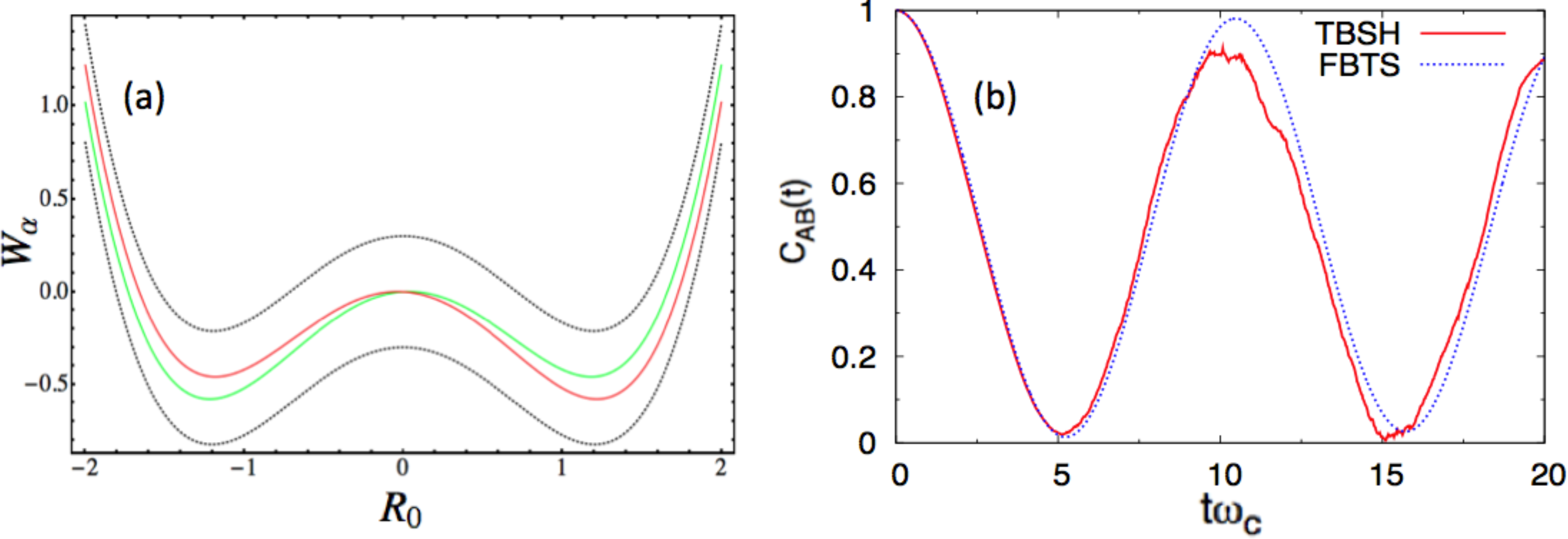
In this study, we report numerical results in the energy unit, ℏωc, and distance unit, , for each environmental DOF. We consider two sets of parameters. In the first case, we use the following parameter values, a = 1.0, ω0 = 1.2, γ0 = 0.05 γb = 1.0, Ω = 0.3, ξ = 0.1, ωmax = 3 and β = 0.2, in the dimensionless units. Figure 1a presents the potential surface profiles [53], Wα(R0). The two diabatic surfaces, WL,R(R0), remain close to each other, and the two adiabatic surfaces, W±(R0), share essentially the same characteristics. In this case, a mean-field-based algorithm, like FBTS, should be accurate and efficient. This problem can also be handled easily in the adiabatic basis, since the surface-hopping trajectories will be initialized in both the adiabatic ground and excited states, because the system is in a thermal equilibrium state at t = 0. Furthermore, the coupling parameter, γb, was purposely chosen to be small in order to minimize the number of nonadiabatic transitions (or hops) encountered in the TBSH algorithm. In panel (b), CLL(t) is computed using both algorithms. The agreement between these results is good.
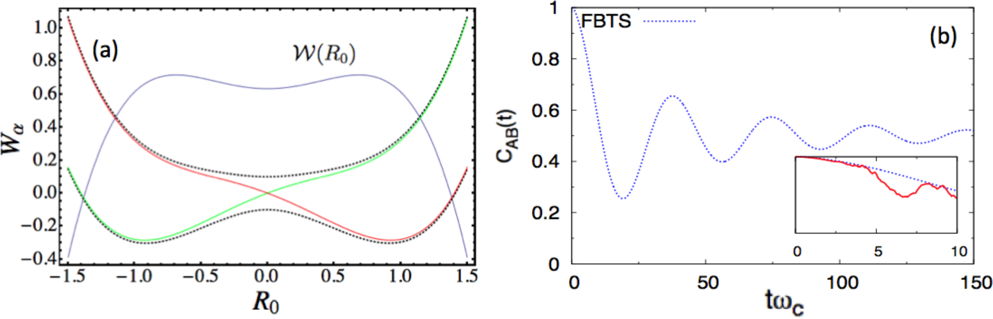
Next, we consider the following parameter set, a = 0.8, ω0 = 0.6, γ0 = 0.3 γb = 1.0, Ω = 0.1, ξ = 0.1, ωmax = 3, and β = 0.2 in the dimensionless units. Figure 2a shows the potential surface profiles, Wα(R0), obtained from this set of parameters. In this case, the adiabatic, W±(R0), and diabatic surfaces, WL,R(R0), only differ markedly near the region of the barrier top, where an avoided crossing point indicates significant mixing of the two diabatic states. Nonadiabatic effects should be most prominent near this barrier top. A stronger coupling, γ0, is also chosen in this case. Figure 2b presents the autocorrelation functions. In the main figure of panel (b), the blue curves (CLL(t) computed by the FBTS) start with the full correlation at one, then gradually reduce to 1/2, which implies that the subsystem is in an equal admixture of the two diabatic states in the asymptotic limit. The TBSH simulation results are only valid for very short times (as shown in the inset of the Figure 2b), due to instability arising from the accumulation of weights, even with filtering [54]. The thermal equilibrium distribution, (R0), has a bimodal distribution profile, as illustrated in Figure 2a; however, for the (inverse) temperature, β = 0.2, the double-peaked structure is very broad. The (R0) distribution profile (blue curve in Figure 2a) suggests that the thermal equilibrium state has a non-trivial contribution from the excited surface. Sampling from (R0) yields many R0 values near the barrier top, where several hops immediately take place for this strong-coupling case, and the instability sets in early in the simulation. Lowering β will produce a more pronounced double-peak structure for (R0), but the quartic oscillator’s momentum, P0, will fluctuate with a larger variance in the presence of the heat bath in this case. Since nonadiabatic transitions depend non-trivially on a = P0· d12(R0)Δt in the TBSH algorithm, large momentum fluctuations will eventually affect the long-time result. This case shows some of the practical limitations of the TBSH algorithm for the computation of this correlation function.
5. Conclusions
The scheme for computing the quantum correlation function in Equation (2) combines a numerically exact quantum initial sampling method with dynamics described by the QCLE; thus, the approximations in the simulation method reside in the dynamics. It is easier to compute the equilibrium properties of a quantum system, for instance, by using the imaginary-time Feynman path integral method, than to obtain dynamical properties by using similar real-time Feynman path integrals without adopting further approximations. Since we approximate the quantum dynamics of the entire system, quantum subsystem plus bath, by QCL dynamics, it is appropriate to comment on some of its features.
It is known that the quantum-classical bracket, defined in terms of the commutator and Poisson brackets in Equation (8), does not possess a Lie algebraic structure, since it fails to satisfy the Jacobi identity [2,38]. This lack of a proper algebraic structure is shared by all known MQC methods and simply reflects the inconsistency in mixing classical and quantum mechanical dynamics. One consequence of this inconsistency is that the partial Wigner transform, ρ̂We(R, P), of the full canonical equilibrium density function, ρ̂eq = e−βĤ/ZQ, is not stationary under the QCLE; however, ρ̂We(R, P) can be written as an expansion in the mass ratio (or ℏ), and it has been shown that the full quantum equilibrium density is conserved under the QCL dynamics up to (ℏ). Therefore, the detailed balance relation is also satisfied to this order. The violation of a detailed balance is a common problem that affects all major MQC methods, including the two most popular approaches, Ehrenfest mean-field [55] and Tully’s fewest switching surface hopping [56] (FSSH), to various degrees. Of course, as noted earlier, for the class of models where an arbitrary quantum system is bilinearly coupled to a harmonic bath, the dynamics is exact, and a detailed balance is exactly satisfied.
The dynamics described by the QCLE can be related to that prescribed by other methods. In [57], it was shown that one could derive both Ehrenfest mean-field dynamics and a version of surface-hopping dynamics starting from the QCLE. In the former case, one simply drops all the “correlations” (including entanglement) between the subsystem and bath densities in the QCLE [58]. In the later case, one projects out all the off-diagonal matrix elements of the density in the QCLE to obtain a generalized master equation for the subsystem alone. Then, one considers decoherence to suppress the coherences in order to recover a simple “surface hopping” dynamics [59] similar to that prescribed in the FSSH algorithm. Furthermore, it had been proven [60] that the QCLE and the partially linearized path integral (PLPI) method [61–64] share the same starting mathematical foundation. In particular, the most recent PLPI algorithm, called PLDM (Partially Linearized Density Matrix) method [64], is very similar to the FBTS presented in this paper [31]. One can also draw comparisons between methods based on the QCLE and semiclassical initial value representations. For instance, numerical schemes based on the Poisson bracket mapping equation (PBME) [30], an approximate equation derived from the mapping-transformed QCLE, and the linearized semiclassical initial value representations [65] share the same set of equations of motion for the trajectories.
Mixed quantum-classical methods are often the only feasible approach to explore the dynamics of large complex systems, such as condensed phase or biochemical systems, where only a few light-mass DOF need be treated quantum mechanically. In many rate processes of interest, such as electron transfer or proton transfer, the local polar solvent motions are responsible for important features of the reaction mechanism. As a result, it is essential that the dynamics of these environmental degrees of freedom be treated in detail. Open quantum system methods that trace out all bath details cannot capture important aspects of such dynamics.
Some recent work [48,66] has suggested interesting ways to combine the QCLE and the generalized master equation [67–69] approach. Simulation tests on spin boson models [48] and a two-level system coupled to an anharmonic bath [68] indicate that accurate, long-time dynamical properties of such systems can be efficiently calculated with an improved memory kernel (which takes the short-time QCLE computation of some bath correlation functions as the input) for the general master equation. This type of hybrid approach may eventually prove to be useful for studies of more complex systems.
Finally, we provide comments that may help in choosing between the two algorithms for simulations. The TBSH algorithm, without filtering, provides a very accurate QCL dynamics before the onset of the sign problem associated with its heavy reliance on Monte Carlo sampling. While filtering can be used to extend simulations to much longer times, the problems related to Monte Carlo sampling limits its usefulness in performing long-time simulations, as vividly illustrated in Section 4. However, the TBSH is found to be the preferred simulation method (in comparison to the FBTS) when one investigates bath dynamical properties of systems in the vicinity of conical intersections and avoided crossings. For instance, the TBSH results accurately capture the intricate geometric phases [46] and the bimodal structure in the momentum distribution [35] in the Tully 1 model (a single avoided crossing model), while the FBTS fails to reproduce these delicate features, even though it provides fairly accurate population dynamics, as reported in [36]. Since the FBTS trajectory dynamics is based on a mean-field description, one finds that the results are usually very accurate (even in the long-time limit) when the energy gap between diabatic energy surfaces is small in comparison to the typical subsystem-bath coupling strength. Another advantage of the FBTS is the availability of the JFBTS [36] algorithm, which implements systematic correction of FBTS results towards the exact QCL dynamics and provides a simple method to gauge the sufficiency of the FBTS results.
Acknowledgments
Research was supported in part by a grant from the Natural Sciences and Engineering Research Council of Canada.
Conflicts of Interest
The authors declare no conflict of interest.
Appendix High Temperature Limit
Many realistic chemical and biological processes take place at room temperature, in which case, it is often justified to apply a classical approximation to the bath. In this Appendix, we make two assumptions: As in most condensed phase models, we consider a pure subsystem observable, Â, such that . We also assume that the environment is further partitioned into an immediate part that can couple nonlinearly to the quantum subsystem and shield the subsystem from the larger set of environmental DOF, often modeled as a heat bath of independent harmonic oscillators. Furthermore, we write X = {Xb, Xn}, where n refers to the few DOF that couple directly to the quantum subsystem and b refers to the remainder of the large number of coordinates that only couple to the n-labeled coordinates. Similarly, we re-label different parts of the Hamiltonian as follows: Ĥ =Ĥs +Ĥn + V̂sn +Ĥb + V̂bn with Ĥi = K̂i+ V̂i and i = s, b, n. The quantities, K̂i and V̂i, are the total kinetic energy and isolated potential, respectively, of the i-th system. Potential energy terms with a subscript of two letters imply a coupling potential between two components of the composite system. In addition, we introduce ĥW (Rn) = Ĥs + V̂sn(Rn) + Vn(Rn),Ĥbn(Rn) = Ĥb + V̂bn(Rn) and Ĥsn =ĥW (Rn) + K̂n. In the following, we express the distance in units of and energy in units of ℏωc, where ωc is the cut-off frequency of the heat bath.
Under these assumptions, one needs to evaluate the partial Wigner transform of e−βĤ alone. In the high temperature limit, we factorize the un-normalized equilibrium density matrix operator, ρ̂ = e−βĤsne−βĤbn. The partial Wigner transform of this approximate density operator reads:
We next apply a symmetric Trotter decomposition to the matrix element of Equation (36):
In this equation, the symmetric Trotter decomposition separates the subsystem potential in ĥW (Rn) into harmonic, , and anharmonic, ΔĤ(Rn) =ĥW (Rn) − Vho(Rn), contributions; furthermore, we define Ĥho = K̂n + V̂ho.
The anharmonic term in Equation (37) can be approximated as follows:
Substituting Equation (37) into Equation (36) and integrating out the Z variable, Equation (36) simplifies to:
References
- Zwanzig, R. Time-correlation functions and transport coefficients in statistical mechanics. Annu. Rev. Phys. Chem 1965, 16, 67–102. [Google Scholar]
- Kapral, R.; Ciccotti, G. A Statistical Mechanical Theory of Quantum Dynamics in Classical Environments. In Bridging Time Scales: Molecular Simulations for the Next Decade; Nielaba, P., Mareschal, M., Ciccotti, G., Eds.; Springer: Berlin, Germany, 2002; pp. 445–472. [Google Scholar]
- Bonella, S.; Monteferrante, M.; Pierleoni, C.; Ciccotti, G. Path integral based calculations of symmetrized time correlation functions. I. J. Chem. Phys 2010, 133, 164104. [Google Scholar]
- Bonella, S.; Monteferrante, M.; Pierleoni, C.; Ciccotti, G. Path integral based calculations of symmetrized time correlation functions. II. J. Chem. Phys 2010, 133, 164105. [Google Scholar]
- Monteferrante, M.; Bonella, S.; Ciccotti, G. Linearized symmetrized quantum time correlation functions calculation via phase pre-averaging. Mol. Phys 2011, 109, 3015–3027. [Google Scholar]
- Redfield, A. The Theory of Relaxation Processes. In Advances in Magnetic Resonance; Waugh, J., Ed.; Academic Press: New York, NY, USA, 1965; Volume 1. [Google Scholar]
- Lindblad, G. On the generators of quantum dynamical semigroups. Commun. Math. Phys 1976, 48, 119–130. [Google Scholar]
- Weiss, U. Quantum Dissipative Systems; World Scientific: Singapore, Singapore, 1999. [Google Scholar]
- Blum, K. Density Matrix Theory and Applications; Plenum: New York, NY, USA, 1981. [Google Scholar]
- Breuer, H.P.; Petruccione, F. The Theory of Open Quantum Systems; Oxford University Press: Oxford, UK, 2007. [Google Scholar]
- Feynman, R.P.; Vernon, J.F.L.. The theory of a general quantum mechanical system interacting with a linear dissipative system. Ann. Phys 1963, 24, 118–173. [Google Scholar]
- Feynman, R.P.; Hibbs, A.R.. Quantum Mechanics and Path Integrals; McGraw-Hill: New York, NY, USA, 1965. [Google Scholar]
- Herman, M.F. Dynamics by semiclassical methods. Annu. Rev. Phys. Chem 1994, 45, 83–111. [Google Scholar]
- Thoss, M.; Wang, H.B.. Semiclassical description of molecular dynamics based on initial-value representation methods. Annu. Rev. Phys. Chem 2004, 55, 299–332. [Google Scholar]
- Kay, K.G. Semiclassical initial value treatments of atoms and molecules. Annu. Rev. Phys. Chem 2005, 56, 255–280. [Google Scholar]
- Tully, J.C. Nonadiabatic Dynamics. In Modern Methods for Multidimensional Dynamics Computations in Chemistry; Thompson, D.L., Ed.; World Scientific: New York, NY, USA, 1998; p. 34. [Google Scholar]
- Kapral, R. Progress in the theory of mixed quantum-classical dynamics. Ann. Rev. Phys. Chem 2006, 57, 129–157. [Google Scholar]
- Kapral, R.; Ciccotti, G. Mixed quantum-classical dynamics. J. Chem. Phys 1999, 110, 8919–8929. [Google Scholar]
- Sergi, A.; Kapral, R. Quantum-classical limit of quantum correlation functions. J. Chem. Phys 2004, 121, 7565–7576. [Google Scholar]
- Nassimi, A.; Kapral, R. Mapping approach for quantum-classical time correlation functions 1. Can. J. Chem 2009, 87, 880–890. [Google Scholar]
- Filinov, V.; Bonella, S.; Lozovik, Y.; Filinov, A.; Zacharov, I. Quantum Molecular Dynamics Using Wigner Representation. In Classical Dynamics in Condensed Phase Simulations; Berne, B.J., Ciccotti, G., Coker, D.C., Eds.; World Scientic: Singapore, Singapore, 1998. [Google Scholar]
- Basire, M.; Borgis, D.; Vuilleumier, R. Computing Wigner distributions and time correlation functions using the quantum thermal bath method: Application to proton transfer spectroscopy. Phys. Chem. Chem. Phys 2013, 15, 12591–12601. [Google Scholar]
- Martens, C.C.; Fang, J.Y.. Semiclassical-limit molecular dynamics on multiple electronic surfaces. J. Chem. Phys 1996, 106, 4918–4930. [Google Scholar]
- Donoso, A.; Martens, C.C.. Simulation of coherent nonadiabatic dynamics using classical trajectories. J. Phys. Chem. A 1998, 102, 4291–4300. [Google Scholar]
- MacKernan, D.; Kapral, R.; Ciccotti, G. Sequential short-time propagation of quantum-classical dynamics. J. Phys. Condens. Matter 2002, 14, 9069–9076. [Google Scholar]
- MacKernan, D.; Ciccotti, G.; Kapral, R. Trotter-based simulation of quantum-classical dynamics. J. Phys. Chem. B 2008, 112, 424–432. [Google Scholar]
- Horenko, I.; Salzmann, C.; Schmidt, B.; Schutte, C. Quantum-classical Liouville approach to molecular dynamics: Surface hopping Gaussian phase-space packets. J. Chem. Phys 2002, 117, 11075–11088. [Google Scholar]
- Wan, C.; Schofield, J. Mixed quantum-classical molecular dynamics: Aspects of the multithreads algorithm. J. Chem. Phys 2000, 113, 7047–7054. [Google Scholar]
- Wan, C.; Schofield, J. Solutions of mixed quantum-classical dynamics in multiple dimensions using classical trajectories. J. Chem. Phys 2002, 116, 494–506. [Google Scholar]
- Kim, H.; Nassimi, A.; Kapral, R. Quantum-classical Liouville dynamics in the mapping basis. J. Chem. Phys 2008, 129, 084102. [Google Scholar]
- Hsieh, C.Y.; Kapral, R. Nonadiabatic dynamics in open quantum-classical systems: Forward-backward trajectory solution. J. Chem. Phys 2012, 137, 22A507. [Google Scholar]
- Stock, G.; Thoss, M. Classical description of nonadiabatic quantum dynamics. Adv. Chem. Phys 2005, 131, 243–375. [Google Scholar]
- Schwinger, J. On Angular Momentum. In Quantum Theory of Angular Momentum; Biedenharn, L.C., Dam, H.V., Eds.; Academic Press: New York, NY, USA, 1965; p. 229. [Google Scholar]
- Nassimi, A.; Bonella, S.; Kapral, R. Analysis of the quantum-classical Liouville equation in the mapping basis. J. Chem. Phys 2010, 133, 134115. [Google Scholar]
- Kelly, A.; van Zon, R.; Schofield, J.; Kapral, R. Mapping quantum-classical Liouville equation: Projectors and trajectories. J. Chem. Phys 2012, 136, 084101. [Google Scholar]
- Hsieh, C.Y.; Kapral, R. Analysis of the forward-backward trajectory solution for the mixed quantum-classical Liouville equation. J. Chem. Phys 2013, 138, 134110. [Google Scholar]
- Ananth, N.; Miller, T.F.. Exact quantum statistics for electronically nonadiabatic systems using continuous path variables. J. Chem. Phys 2010, 133, 234103. [Google Scholar]
- Nielsen, S.; Kapral, R.; Ciccotti, G. Statistical mechanics of quantum-classical systems. J. Chem. Phys 2001, 115, 5805–5815. [Google Scholar]
- Kim, H.; Hanna, G.; Kapral, R. Analysis of kinetic isotope effects for nonadiabatic reactions. J. Chem. Phys 2006, 125, 084509. [Google Scholar]
- Hanna, G.; Kapral, R. Quantum-classical Liouville dynamics of nonadiabatic proton transfer. J. Chem. Phys 2005, 122, 244505. [Google Scholar]
- Kim, H.; Kapral, R. Solvation and proton transfer in polar molecule nanoclusters. J. Chem. Phys 2005, 125, 234309. [Google Scholar]
- Kim, H.; Kapral, R. Proton and deuteron transfer reactions in molecular nanoclusters. ChemPhysChem 2008, 9, 470–474. [Google Scholar]
- Hanna, G.; Geva, E. Vibrational energy relaxation of a hydrogen-bonded complex dissolved in a polar liquid via the mixed quantum-classical lionville method. J. Phys. Chem. B 2008, 112, 4048–4058. [Google Scholar]
- Horenko, I.; Schmidt, B.; Schutte, C. A theoretical model for molecules interacting with intense laser pulses: The floquet-based quantum-classical Liouville equation. J. Chem. Phys 2001, 115, 5733–5743. [Google Scholar]
- Morales, C.M.; Thompson, W.H.. Mixed quantum-classical molecular dynamics analysis of the molecular-level mechanisms of vibrational frequency shifts. J. Phys. Chem. A 2007, 111, 5422–5433. [Google Scholar]
- Kelly, A.; Kapral, R. Quantum-classical description of environmental effects on electronic dynamics at conical intersections. J. Chem. Phys 2010, 133, 084502. [Google Scholar]
- Kim, H.W.; Kelly, A.; Park, J.W.; Rhee, Y.M.. All-atom semiclassical dynamics study of quantum coherence in photosynthetic fennamatthewsolson complex. J. Am. Chem. Soc 2012, 134, 11640–11651. [Google Scholar]
- Kelly, A.; Markland, T.E.. Efficient and accurate surface hopping for long time nonadiabatic quantum dynamics. J. Chem. Phys 2013, 139, 014104. [Google Scholar]
- Stock, G.; Thoss, M. Semiclassical description of nonadiabatic quantum dynamics. Phys. Rev. Lett 1997, 78, 578–581. [Google Scholar]
- Ananth, N.; Venkataraman, C.; Miller, W.H.. Semiclassical description of electronically nonadiabatic dynamics via the initial value representation. J. Chem. Phys 2007, 127, 084114. [Google Scholar]
- Huo, P.; Coker, D.F.. Consistent schemes for non-adiabatic dynamics derived from partial linearized density matrix propagation. J. Chem. Phys 2012, 137, 22A535. [Google Scholar]
- Makri, N.; Thompson, K. Semiclassical influence functionals for quantum systems in anharmonic environments. Chem. Phys. Lett 1998, 291, 101–109. [Google Scholar]
- Sergi, A.; Kapral, R. Quantum-classical dynamics of nonadiabatic chemical reactions. J. Chem. Phys 2003, 118, 8566–8575. [Google Scholar]
- Bonella, S.; Coker, D.F.; Kernan, D.M.; Kapral, R.; Ciccotti, G. Trajectory Based Simulations of Quantum-Classical Systems. In Energy Transfer Dynamics in Biomaterial Systems; Burghardt, I., May, V., Micha, D.A., Bittner, E.R., Eds.; Springer: Berlin/Heidelberg, Germany, 2009; Volume 93. [Google Scholar]
- Parandekar, P.V.; Tully, J.C.. Mixed quantum-classical equilibrium. J. Chem. Phys 2005, 122, 094102. [Google Scholar]
- Schmidt, J.R.; Parandekar, P.V.; Tully, J.C.. Mixed quantum-classical equilibrium: Surface hopping. J. Chem. Phys 2008, 129, 044104. [Google Scholar]
- Grunwald, R.; Kelly, A.; Kapral, R. Quantum Dynamics in Almost Classical Environments. In Energy Transfer Dynamics in Biomaterial Systems; Springer: Berlin/Heidelberg, Germany, 2009; pp. 383–413. [Google Scholar]
- Gerasimenko, V.I. Dynamical equations of quantum-classical systems. Theor. Math. Phys 1982, 50, 49–55. [Google Scholar]
- Grunwald, R.; Kapral, R. Decoherence and quantum-classical master equation dynamics. J. Chem. Phys 2007, 126, 114109. [Google Scholar]
- Bonella, S.; Ciccotti, G.; Kapral, R. Linearization approximation and Liouville Quantum-classical dynamics. Chem. Phys. Lett 2010, 484, 399–404. [Google Scholar]
- Bonella, S.; Coker, D.F.. Semiclassical implementation of the mapping Hamiltonian approach for nonadiabatic dynamics using focused initial distribution sampling. J. Chem. Phys 2003, 118, 4370–4385. [Google Scholar]
- Bonella, S.; Coker, D.F.. LAND-map, a linearized approach to nonadiabatic dynamics using the mapping formalism. J. Chem. Phys 2005, 122, 194102. [Google Scholar]
- Dunkel, E.; Bonella, S.; Coker, D.F.. Iterative linearized approach to nonadiabatic dynamics. J. Chem. Phys 2008, 129, 114106. [Google Scholar]
- Huo, P.; Coker, D.F.. Partial linearized density matrix dynamics for dissipative, non-adiabatic quantum evolution. J. Chem. Phys 2011, 135, 201101. [Google Scholar]
- Liu, J.; Miller, W.H.. Real time correlation function in a single phase space integral beyond the linearized semiclassical initial value representation. J. Chem. Phys 2007, 126, 234110. [Google Scholar]
- Shi, Q.; Geva, E. A derivation of the mixed quantum-classical Liouville equation from the influence functional formalism. J. Chem. Phys 2004, 121, 3393–3404. [Google Scholar]
- Shi, Q.; Geva, E. A new approach to calculating the memory kernel of the generalized quantum master equation for an arbitrary systembath coupling. J. Chem. Phys 2003, 119, 12063–12076. [Google Scholar]
- Shi, Q.; Geva, E. A semiclassical generalized quantum master equation for an arbitrary system-bath coupling. J. Chem. Phys 2004, 120, 10647–10658. [Google Scholar]
- Zhang, M.L.; Ka, B.J.; Geva, E. Nonequilibrium quantum dynamics in the condensed phase via the generalized quantum master equation. J. Chem. Phys 2006, 125, 044106. [Google Scholar]
- Kim, H.; Kapral, R. Nonadiabatic quantum-classical reaction rates with quantum equilibrium structure. J. Chem. Phys 2005, 123, 194108. [Google Scholar]


© 2014 by the authors; licensee MDPI, Basel, Switzerland This article is an open access article distributed under the terms and conditions of the Creative Commons Attribution license (http://creativecommons.org/licenses/by/3.0/).
Share and Cite
Hsieh, C.-Y.; Kapral, R. Correlation Functions in Open Quantum-Classical Systems. Entropy 2014, 16, 200-220. https://0-doi-org.brum.beds.ac.uk/10.3390/e16010200
Hsieh C-Y, Kapral R. Correlation Functions in Open Quantum-Classical Systems. Entropy. 2014; 16(1):200-220. https://0-doi-org.brum.beds.ac.uk/10.3390/e16010200
Chicago/Turabian StyleHsieh, Chang-Yu, and Raymond Kapral. 2014. "Correlation Functions in Open Quantum-Classical Systems" Entropy 16, no. 1: 200-220. https://0-doi-org.brum.beds.ac.uk/10.3390/e16010200