Malliavin Weight Sampling: A Practical Guide

Abstract
: Malliavin weight sampling (MWS) is a stochastic calculus technique for computing the derivatives of averaged system properties with respect to parameters in stochastic simulations, without perturbing the system’s dynamics. It applies to systems in or out of equilibrium, in steady state or time-dependent situations, and has applications in the calculation of response coefficients, parameter sensitivities and Jacobian matrices for gradient-based parameter optimisation algorithms. The implementation of MWS has been described in the specific contexts of kinetic Monte Carlo and Brownian dynamics simulation algorithms. Here, we present a general theoretical framework for deriving the appropriate MWS update rule for any stochastic simulation algorithm. We also provide pedagogical information on its practical implementation.1. Introduction
Malliavin weight sampling (MWS) is a method for computing derivatives of averaged system properties with respect to parameters in stochastic simulations [1,2]. The method has been used in quantitative financial modelling to obtain the “Greeks” (price sensitivities) [3], and as the Girsanov transform, in kinetic Monte Carlo simulations for systems biology [4]. Similar ideas have been used to study fluctuation-dissipation relations in supercooled liquids [5]. However, MWS appears to be relatively unknown in the fields of soft matter, chemical and biological physics, perhaps because the theory is relatively impenetrable for non-specialists, being couched in the language of abstract mathematics (e.g., martingales, Girsanov transform, Malliavin calculus, etc.); an exception in financial modelling is [6].
MWS works by introducing an auxiliary stochastic quantity, the Malliavin weight, for each parameter of interest. The Malliavin weights are updated alongside the system’s usual (unperturbed) dynamics, according to a set of rules. The derivative of any system function, A, with respect to a parameter of interest is then given by the average of the product of A with the relevant Malliavin weight; or in other words, by a weighted average of A, in which the weight function is given by the Malliavin weight. Importantly, MWS works for non-equilibrium situations, such as time-dependent processes or driven steady states. It thus complements existing methods based on equilibrium statistical mechanics, which are widely used in soft matter and chemical physics.
MWS has so far been discussed only in the context of specific simulation algorithms. In this paper, we present a pedagogical and generic approach to the construction of Malliavin weights, which can be applied to any stochastic simulation scheme. We further describe its practical implementation in some detail using as our example one dimensional Brownian motion in a force field.
2. The Construction of Malliavin Weights
The rules for the propagation of Malliavin weights have been derived for the kinetic Monte-Carlo algorithm [4,7], for the Metropolis Monte-Carlo scheme [5] and for both underdamped and overdamped Brownian dynamics [8]. Here we present a generic theoretical framework, which encompasses these algorithms and also allows extension to other stochastic simulation schemes.
We suppose that our system evolves in some state space, and a point in this state space is denoted as S. Here, we assume that the state space is continuous, but our approach can easily be translated to discrete or mixed discrete-continuous state spaces. Since the system is stochastic, its state at time t is described by a probability distribution, P (S). In each simulation step, the state of the system changes according to a propagator, W (S → S′), which gives the probability that the system moves from point S to point S′ during an application of the update algorithm. The propagator has the property that
Let us now consider the average of some quantity A(S) over the state space, in shorthand
Let us now suppose that we track in our simulation not only the physical state of the system, but also an auxiliary stochastic variable, which we term qλ. At each simulation step qλ is updated according to a rule that depends on the system state; this does not perturb the system’s dynamics, but merely acts as a “readout”. By tracking qλ, we extend the state space, so that S becomes {S, qλ}. We can then define the average 〈qλ〉S, which is an average of the value of qλ in the extended state space, with the constraint that the original (physical) state space point is fixed at S (see further below).
Our aim is to define a set of rules for updating qλ, such that 〈qλ〉S = Qλ, i.e., such that the average of the auxiliary variable, for a particular state space point, measures the derivative of the probability distribution with respect to the parameter of interest, λ. If this is the case then, from Equation (5)
How do we go about finding the correct updating rule? If the Malliavin weight exists, we should be able to derive its updating rule from the system’s underlying stochastic equations of motion. We obtain an important clue from differentiating Equation (1) with respect to λ. Extending the shorthand notation, one finds
From a practical point of view, for each time step, we implement the following procedure:
propagate the system from its current state S to a new state S′ using the algorithm that implements the stochastic equations of motion (Brownian, kinetic Monte-Carlo, etc.);
with knowledge of S and S′, and the propagator W (S → S′), calculate the change in the Malliavin weight Δqλ = ∂ ln W (S → S′)/∂λ;
update the Malliavin weight according to qλ → q′λ = qλ+ Δqλ.
At the start of the simulation, the Malliavin weight is usually initialised to qλ = 0.
Let us first suppose that our system is not in steady state. However rather the quantity 〈A〉 in which we are interested is changing in time and likewise ∂〈A(t)〉/∂λ is a time-dependent quantity. To compute ∂〈A(t)〉/∂λ we run N independent simulations, in each one tracking as a function of time A(t), qλ(t) and the product A(t) qλ(t). The quantities 〈A(t)〉 and ∂〈A(t)〉/∂λ are then given by
If, instead, our system is in steady state, the procedure needs to be modified slightly. This is because the variance in the values of q (t) across replicate simulations increases linearly in time (this point is discussed further below). For long times, computation of ∂〈A〉/∂λ using Equation (10) therefore incurs a large statistical error. Fortunately, this problem can easily be solved by computing the correlation function
Returning to a more theoretical perspective, it is interesting to note that the rule for updating the Malliavin weight, Equation (9), depends deterministically on S and S′. This implies that the value of the Malliavin weight at time t is completely determined by the trajectory of system states during the time interval 0 → t. In fact, it is easy to show that
3. Multiple Variables, Second Derivatives and the Algebra of Malliavin Weights
Up to now, we have assumed that the quantity A does not depend explicitly on the parameter λ. There may be cases, however, when A does have an explicit λ-dependence. In these cases, Equation (7) should be replaced by
We can also extend our analysis further to allow us to compute higher derivatives with respect to the parameters. These may be useful, for example, for increasing the efficiency of gradient-based parameter optimisation algorithms. Taking the derivative of Equation (13) with respect to a second parameter μ gives
Steady state problems can be approached by extending the correlation function method to second order weights. Define, cf. Equation (11),
As in the first order case, in steady state we expect C(t, t′) = C(t − t′) with the property that C(Δt) → ∂2〈A〉/∂λ∂μ as Δt → ∞.
4. One-Dimensional Brownian Motion in a Force Field
We now demonstrate this machinery by way of a practical but very simple example, namely one-dimensional (overdamped) Brownian motion in a force field. In this case, the state space is specified simply by the particle position x which evolves according to the Langevin equation
If we differentiate Equation (23) with respect to a second parameter μ we get
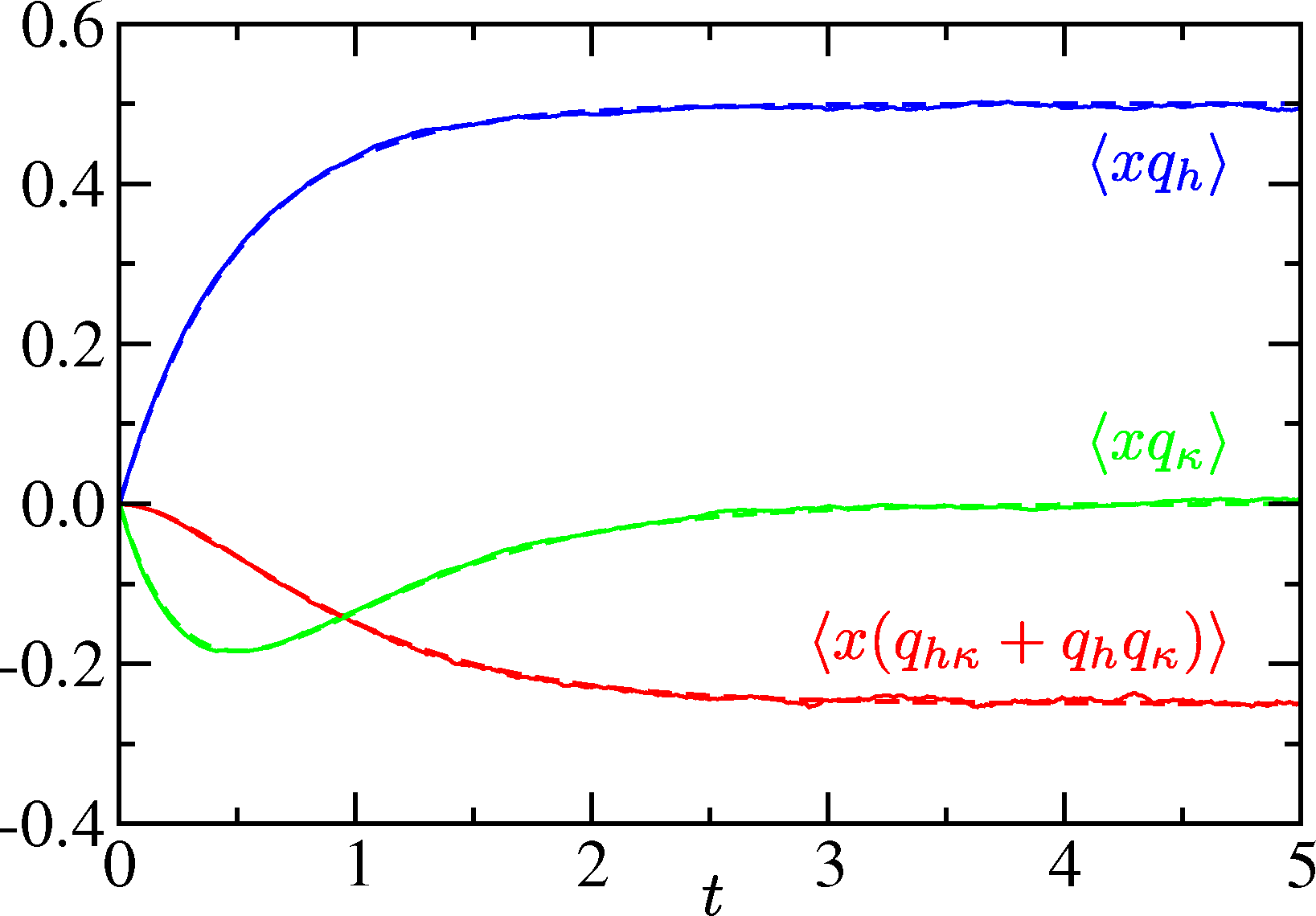
Now let us consider the simplest case of a particle in a linear force field f = −κx + h (also discussed in [8]). This corresponds to a harmonic trap with the potential . We let the particle start from x0 at t = 0 and track its time-dependent relaxation to the steady state. We shall set T = 1 for simplicity. The Langevin equation can be solved exactly for this case, and the mean position evolves according to
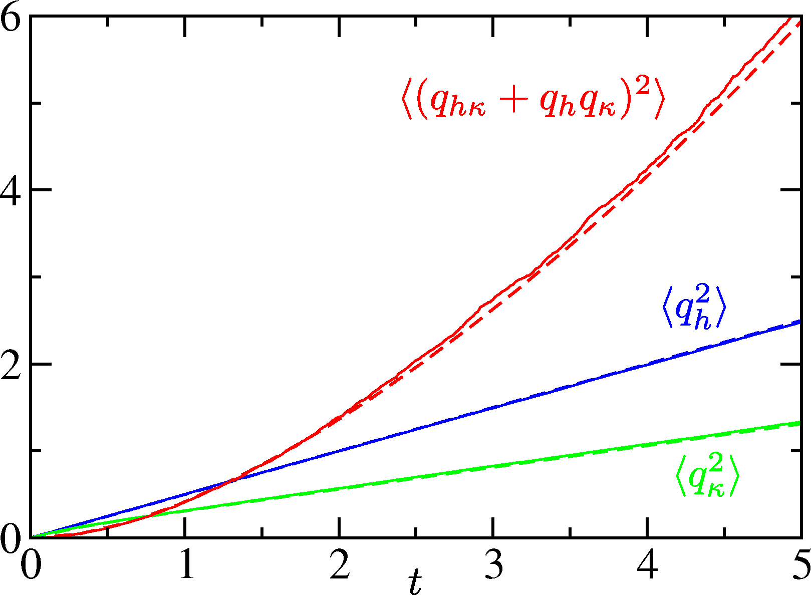
As discussed briefly above, in this procedure the sampling error in the computation of ∂〈A(t)〉/∂λ is expected to grow with time. Figure 2 shows the mean square Malliavin weight as a function of time for the same problem. For the first order weights qh and qκ the growth rate is typically linear in time. Indeed, from Equation (29), one can prove that in the limit δt → 0 (see Section 5)
5. Conclusions
In this paper, we have provided an outline of the generic use of Malliavin weights for sampling derivatives in stochastic simulations, with an emphasis on practical aspects. The usefulness of MWS for a particular simulation scheme hinges on the simplicity or otherwise of constructing the propagator W (S → S′) which fixes the updating rule for the Malliavin weights according to Equation (9). The propagator is determined by the algorithm used to implement the stochastic equations of motion; MWS may be easier to implement for some algorithms than for others. We note however that there is often some freedom of choice about the algorithm, such as the choice of a stochastic thermostat in molecular dynamics, or the order in which update steps are implemented. In these cases, a suitable choice may simplify the construction of the propagator and facilitate the use of Malliavin weights.
Acknowledgments
Rosalind J. Allen is supported by a Royal Society University Research Fellowship.
Conflicts of Interest
The authors declare no conflict of interest.
References
- Bell, D.R. The Malliavin Calculus; Dover: Mineola, NY, USA, 2006. [Google Scholar]
- Nualart, D. The Malliavin Calculus and Related Topics; Springer: New York, NY, USA, 2006. [Google Scholar]
- Fournié, E.; Lasry, J.M.; Lebuchoux, J.; Lions, P.L.; Touzi, N. Applications of Malliavin calculus to Monte Carlo methods in finance. Financ. Stoch 1999, 3, 391–412. [Google Scholar]
- Plyasunov, A.; Arkin, A.P. Efficient stochastic sensitivity analysis of discrete event systems. J. Comput. Phys 2007, 221, 724–738. [Google Scholar]
- Berthier, L. Efficient measurement of linear susceptibilities in molecular simulations: Application to aging supercooled liquids. Phys. Rev. Lett 2007, 98, 220601. [Google Scholar]
- Chen, N.; Glasserman, P. Malliavin Greeks without Malliavin calculus. Stoch. Proc. Appl 2007, 117, 1689–1723. [Google Scholar]
- Warren, P.B.; Allen, R.J. Steady-state parameter sensitivity in stochastic modeling via trajectory reweighting. J. Chem. Phys 2012, 136, 104106. [Google Scholar]
- Warren, P.B.; Allen, R.J. Malliavin weight sampling for sensitivity coefficients in Brownian dynamics simulations. Phys. Rev. Lett 2012, 109, 250601. [Google Scholar]
- Warren, P.B.; ten Wolde, P.R. Chemical models of genetic toggle switches. J. Phys. Chem. B 2005, 109, 6812–6823. [Google Scholar]
Appendix
MATLAB Script
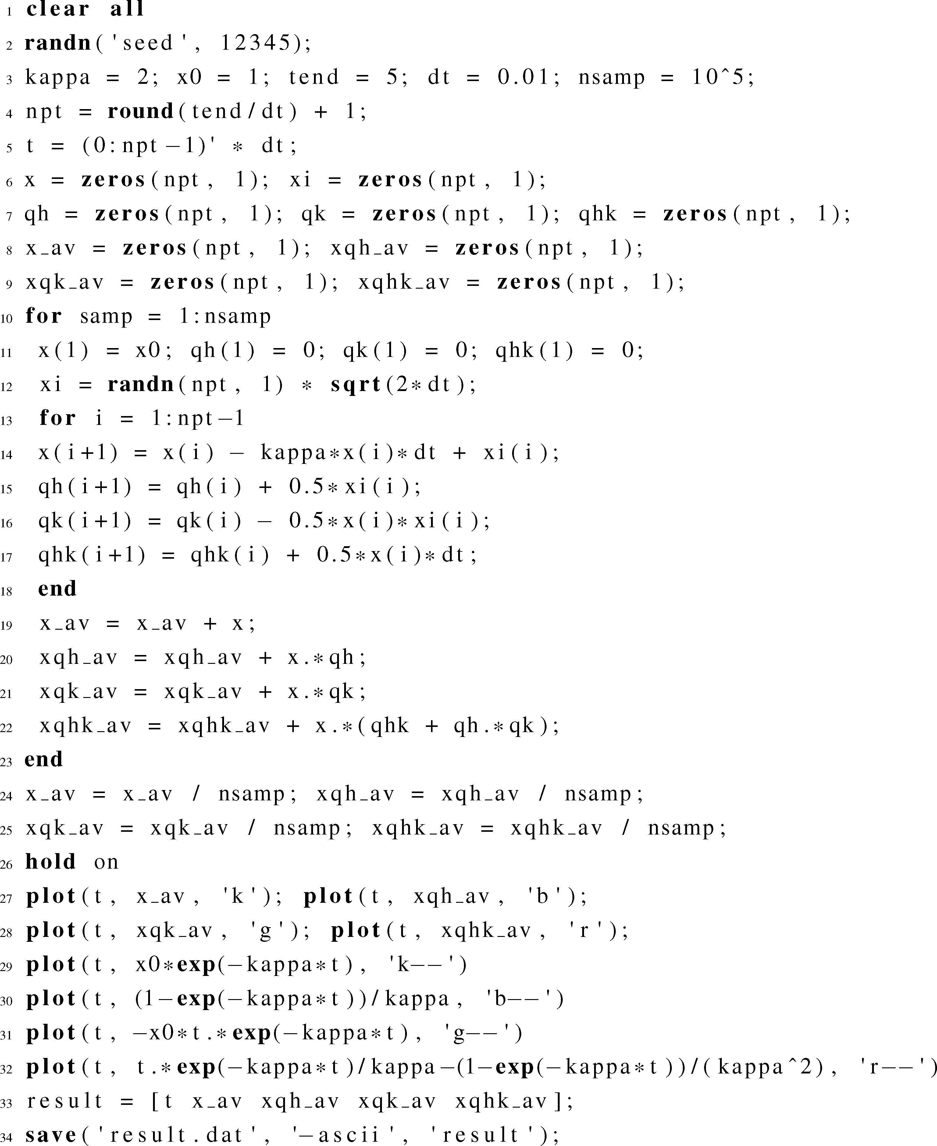
The MATLAB script in Listing 1 was used to generate the results shown in Figure 1. It implements Equations (29)–(31) above, making extensive use of the compact MATLAB syntax for array operations, for instance invoking ‘.*’ for element-by-element multiplication of arrays.

Here is a brief explanation of the script. Lines 1–3 initialise the problem and the parameter values. Lines 4 and 5 calculate the number of points in a trajectory and initialise a vector containing the time coordinate of each point. Lines 6–9 set aside storage for the actual trajectory, Malliavin weights and cumulative statistics. Lines 10–23 implement a pair of nested loops, which are the kernel of the simulation. Within the outer (trajectory sampling) loop, Line 11 initialises the particle position and Malliavin weights, Line 12 precomputes a vector of random displacements (Gaussian random variates), and Lines 13–18 generate the actual trajectory. Within the inner (trajectory generating loop), Lines 14–17 are a direct implementation of Equations (29) and (30). After each individual trajectory has been generated, the cumulative sampling step implied by Equation (31) is done in Lines 19–22; after all the trajectories have been generated, these quantities are normalised in Lines 24 and 25. Finally, Lines 26–32 generate a plot similar to Figure 1 (albeit with the addition of 〈x〉), and Lines 33 and 34 show how the data can be exported in tabular format for replotting using an external package.
Listing 1 is complete and self-contained. It will run in either MATLAB or Octave. One minor comment is perhaps in order. The choice was made to precompute a vector of Gaussian random variates, which are used as random displacements to generate the trajectory and update the Malliavin weights. One could equally well generate random displacements on-the-fly, in the inner loop. For this one-dimensional problem storage is not an issue and it seems more elegant and efficient to exploit the vectorisation capabilities of MATLAB. For a more realistic three-dimensional problem, with many particles (and a different programming language), it is obviously preferable to use an on-the-fly approach.
Selected Analytic Results
Here, we present analytic results for the growth in time of the mean square Malliavin weights. We can express the rate of growth of the mean of a generic function f(x, qh, qκ, qhκ) as


© 2014 by the authors; licensee MDPI, Basel, Switzerland This article is an open access article distributed under the terms and conditions of the Creative Commons Attribution license (http://creativecommons.org/licenses/by/3.0/).
Share and Cite
Warren, P.B.; Allen, R.J. Malliavin Weight Sampling: A Practical Guide. Entropy 2014, 16, 221-232. https://0-doi-org.brum.beds.ac.uk/10.3390/e16010221
Warren PB, Allen RJ. Malliavin Weight Sampling: A Practical Guide. Entropy. 2014; 16(1):221-232. https://0-doi-org.brum.beds.ac.uk/10.3390/e16010221
Chicago/Turabian StyleWarren, Patrick B., and Rosalind J. Allen. 2014. "Malliavin Weight Sampling: A Practical Guide" Entropy 16, no. 1: 221-232. https://0-doi-org.brum.beds.ac.uk/10.3390/e16010221