Computing Equilibrium Free Energies Using Non-Equilibrium Molecular Dynamics

Abstract

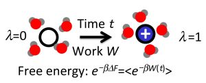
As shown by Jarzynski, free energy differences between equilibrium states can be expressed in terms of the statistics of work carried out on a system during non-equilibrium transformations. This exact result, as well as the related Crooks fluctuation theorem, provide the basis for the computation of free energy differences from fast switching molecular dynamics simulations, in which an external parameter is changed at a finite rate, driving the system away from equilibrium. In this article, we first briefly review the Jarzynski identity and the Crooks fluctuation theorem and then survey various algorithms building on these relations. We pay particular attention to the statistical efficiency of these methods and discuss practical issues arising in their implementation and the analysis of the results.

1. Introduction

The calculation of free energies from atomistic simulations is of great importance in many applications, ranging from the prediction of the phase behavior of a certain substance to the calculation of ligand affinities in drug design. Since the computation of free energies (or, more precisely, of free energy differences) involves the determination of entropic contributions and, hence, the estimation of phase space volumes [1], free energy calculations are computationally very demanding in most cases. Therefore, a significant effort has been devoted to the development of more efficient free energy calculation algorithms. This endeavor has received new momentum with Jarzynski’s discovery of a very general relation between equilibrium free energies and non-equilibrium work [2,3], which has inspired several molecular dynamics-based algorithms for free energy computations. In this article, we will give an overview of these methods.

According to the maximum work theorem, a consequence of the second law of thermodynamics, the amount of work W performed on a system during a non-equilibrium transformation is larger than the free energy difference ΔF between the equilibrium states corresponding to the transition end points:

$$\langle W\rangle \ge \Delta F$$

(1)

Equivalently, the amount of work that can be extracted from a system is bounded from above by the free energy difference. In the above equation, the equal sign holds only if the transformation is carried out reversibly, maintaining equilibrium at all times. The angular brackets on the left-hand side of the maximum work theorem indicate an average over many realizations of the non-equilibrium process. If one considers a macroscopic system, for instance, a piston compressing a gas enclosed in a cylinder, the average is not necessary, because every realization of the process yields, for all practical purposes, the same amount of work W, if the transformation is carried out following the same protocol. This is essentially a consequence of the central limit theorem for thermal fluctuations. In the case of a microscopic system, however, fluctuations become important, and different realizations of the transformation typically produce different work values, leading to a statistical distribution of W. For instance, stretching a biomolecule with atomic force microscopes or optical tweezers will cost a different amount work for each repetition of the experiment. In some cases, the work expended on the system might even be smaller than the free energy difference, seemingly violating the maximum work theorem and, hence, the second law of thermodynamics.

As shown by Jarzynski in 1997 [2,3], the work fluctuations resulting for microscopic systems can be accounted for in an exact way, transforming the maximum work theorem into an equality:

$$\langle e^{-\beta W}\rangle =e^{-\beta \Delta F}$$

(2)

Here, β = 1/k_BT is the reciprocal temperature of the equilibrium state from which the transformation is started, and k_B is the Boltzmann constant. Remarkably, this result, now commonly referred to as Jarzynski equation or Jarzynski non-equilibrium work theorem, relates the statistics of irreversible work carried out on the system, while it is driven away from equilibrium, to an equilibrium free energy difference. A closely connected result is the Crooks fluctuation theorem [4–6], which relates the equilibrium free energy difference to the work distributions of the forward and reversed process.

In general, processes during which work is performed on or by the system drive the system away from equilibrium, such that the phase space distribution obtained at the end of the process may differ strongly from the equilibrium distribution to which the system relaxes after the external perturbation has been stopped. For instance, a piston pushed quickly into a gas-filled cylinder generates non-equilibrium states with strong flows markedly different from the static equilibrium state to which the gas eventually relaxes after the piston has reached its final state. At first sight, it is therefore surprising that equilibrium properties, such as free energy differences, can be extracted from non-equilibrium trajectories. As discussed in the following sections of this paper, a closer analysis reveals that averaging over the work exponential is equivalent to removing the bias introduced during the driving process. It is this unbiasing that ultimately permits the extraction of equilibrium properties (as we will discuss in Section 5, in principle, one can determine the entire equilibrium distribution and not only the free energy) from non-equilibrium trajectories. Thus, the non-equilibrium work theorem can be viewed as a prescription of how to compensate for the effects of manipulations that drive the system into non-equilibrium rather than a tool that illuminates the nature of non-equilibrium processes. Nevertheless, it is remarkable that the bias has a very simple exponential form and can be expressed in terms of the work only.

The Jarzynski non-equilibrium work theorem, as well as the Crooks fluctuation theorem provide the framework for the interpretation of single-molecule pulling experiments [7–9], in which non-equilibrium effects can never be fully avoided. These exact results can also be exploited to devise computer simulation algorithms for the calculation of free energies. In this article, we review several computational approaches based on the collection of work statistics in a fast-switching non-equilibrium setting, paying particular attention to the accuracy and efficient implementation of these methods compared to conventional free energy computation methods (see [10–12]). In the remainder of this article, we will first state the Jarzynski and Crooks theorems more explicitly and discuss the conditions under which they apply. After that, we will survey several fast switching algorithms in which free energies are determined from sets of molecular dynamics trajectories obtained while changing a control parameter, thereby exerting work on the system. We conclude with a brief summary and outlook to future possibilities and applications.

2. Jarzynski Identity and Crooks Fluctuation Theorem

To set the notation, consider a classical system with energy H(x, λ) depending on the microscopic state x of the system, as well as on a parameter λ. The microscopic state x is specified by the positions of all particles in the system and, if necessary, also by all momenta. The parameter λ is a control parameter that can be changed externally, for instance, the volume of the cylinder containing the particles or an external field. According to the basic laws of statistical mechanics, the free energy difference between the two equilibrium states A and B corresponding to the values λ_A and λ_B, respectively, of the order parameter is given by:

$$\Delta F=F_B-F_A=-k_{\text{B}}T\text{ln}\frac{Z_B}{Z_A}$$

(3)

where Z_A = ∫ dx exp{−βH(x, λ_A)} and Z_B = ∫ dx exp{−βH(x, λ_B)} are the canonical partition functions of the two equilibrium states (up to a combinatorial prefactor irrelevant for our considerations). The free energy difference ΔF is the work required to change the external parameter from λ_A to λ_B in a reversible process. Such a reversible transformation could be realized, for instance, by changing the parameter λ infinitely slowly, while keeping the system in contact with a heat bath. In this case, the free energy difference is equal to the work of the system.

Instead of changing the control parameter λ very slowly, one could change it at a finite rate over a time interval τ, following a certain protocol λ(t), where λ(0) = λ_A and λ(τ) = λ_B. In general, such a fast switching of the control parameter drives the system away from equilibrium in an irreversible way, such that the work required to do the change exceeds the free energy difference, as posited by the maximum work theorem of Equation (1). To be more specific, the work performed on the system along a particular trajectory x(t) is the energy change caused by changes of the control parameter accumulated along the trajectory:

$$W[x(t),\lambda (t)]={\int }_0^{\tau }{\frac{\partial H(x(t),\lambda )}{\partial \lambda }|}_{\lambda =\lambda (t)}\dot{\lambda }(t)\hspace{0.17em}\hspace{0.17em}dt$$

(4)

where λ̇(t) is the time derivative of λ(t). Note that this work depends both on the protocol λ(t) as well as on the particular trajectory x(t) followed by the system. The average appearing on the left-hand side of Equation (1) is over many repetitions of the switching process starting from initial conditions distributed according to the equilibrium distribution ρ(x) ∝ exp(−βH(x, λ_A)) for control parameter λ_A. In a computer simulation, one could realize such a process by sampling initial conditions from a canonical distribution and then integrating the underlying equations of motion, while at the same time changing the control parameter λ according to the protocol λ(t).

Jarzynski has shown [2,3] that averaging over the exponential of the work exp(−βW (τ)) rather than the work, turns the maximum work theorem into an equality, 〈exp{−βW[x(t), λ(t)]}〉 = exp{− βΔF}. It is important to realize that the average over the work exponential involves two averages, one over the distribution of initial conditions and another one over the set of trajectories that originate from a particle initial condition. For deterministic dynamics, the initial condition determines the entire trajectory, x(t), but for stochastic dynamics, the system evolves in different ways, even if one repeatedly starts from the same initial condition. Hence, for stochastic dynamics, the average appearing in the Jarzynski equation also requires an average over noise histories.

The Jarzynski equation is an exact result that holds under very general conditions. The requirements are that initially, the system must be in equilibrium and that for a fixed control parameter, the dynamics conserves the equilibrium distribution corresponding to that value of the control parameter. The latter condition is satisfied by most types of dynamics usually used in computer simulations, including Newtonian, thermostated, Langevin and Monte Carlo dynamics. It is worth pointing out that it is not necessary that the system be in an equilibrium state at the end of the transformation process or relax towards equilibrium after the control parameter switching is completed. Furthermore, it is interesting that the Jarzynski equation holds, even if the switching is carried out according to different (though prescribed) protocols provided that λ(0) = λ_A and λ(τ) = λ_B, i.e., all protocols start at λ_A at time 0 and finish at λ_B at time τ. After Jarzynski’s seminal work [2], in which the Jarzynski equality was derived for systems evolving deterministically with and without coupling to a heat bath, several other proofs were provided, for instance, based on a master equation [3], for Markovian dynamics satisfying detailed balance [5,13], for dynamical systems conserving the canonical distribution [14] or from the Feynman–Kac theorem [7].

In the limiting cases of infinitely fast switching and infinitely slow switching, the Jarzynski equality reduced to two well-known results. For instantaneous switching, τ → 0, the initial and final point of a trajectory are identical, as the system has no time to evolve. In this case, the work carried out on the system at a particular microscopic state x equals the difference in energy evaluated for the two values of the control parameter:

$$W(x)=H(x,\hspace{0.17em}{\lambda }_B)-H(x,\hspace{0.17em}{\lambda }_A)$$

(5)

The Jarzynski equation then becomes:

$$e^{-\beta \Delta F}={\langle e^{-\beta [H(x,\hspace{0.17em}{\lambda }_B)-H(x,\hspace{0.17em}{\lambda }_A)]}\rangle }_{{\lambda }_A}$$

(6)

where the subscript next to the angular bracket indicates that the average has to be carried out with respect to the equilibrium distribution at λ_A. The above equation is the central result of free energy perturbation theory [15] and is often used to compute free energy differences. In the opposite limit of infinitely slow switching, τ → ∞, the system has time to equilibrate for every intermediate value of the control parameter, such that the Jarzynski equation together with Equation (4) implies:

$$\Delta F={\int }_{{\lambda }_A}^{{\lambda }_B}{\langle \frac{\partial H(x,\hspace{0.17em}\lambda )}{\partial \lambda }\rangle }_{\lambda }d\lambda$$

(7)

This expression provides the basis for the thermodynamic integration method [16], in which equilibrium simulations are carried out for different, but fixed values of the control parameter λ to compute the average energy derivatives 〈∂H/∂λ〉_λ. The free energy difference is then obtained by numerical integration, for instance, by using the Simpson rule or more sophisticated integration schemes. The maximum work theorem of Equation (1) also immediately follows from the Jarzynski equation by virtue of Jensen’s inequality, 〈exp(−x) 〉 ≥ exp(−〈x〉).

As mentioned in the introduction, the Jarzynski equation can be viewed as a way to remove the bias introduced by the switching process into the phase space distribution obtained at the end of the process. Following similar considerations as those used to derive the Jarzynski equality, one can prove that for any phase space function A(x) the following equation holds [4,7,17]:

$${\langle A(x)\rangle }_{\text{eq},{\lambda }_B}={\langle A(x(\tau ))e^{-\beta [W(\tau )-\Delta F]}\rangle }_{\text{non}-\text{eq}}$$

(8)

Here, the angular brackets on the left-hand side indicate an equilibrium average for the control parameter fixed at λ_B, and the average on the right-hand side is an average over non-equilibrium pathways generated with protocol λ(t) just as in the Jarzynski equations. To make this difference even more explicit, we have added the subscripts eq and non-eq to the equilibrium and non-equilibrium average, respectively. In the above equation, x(τ) refers to the endpoints of the non-equilibrium trajectories. The Jarzynski equation is simply obtained by setting A(x) = 1. Equation (8) implies that equilibrium averages can be computed by reweighting the non-equilibrium distribution obtained as a result of the switching procedure by exp(−βW + βΔF). In particular, the equilibrium distribution for λ_B is obtained by setting A(x) = δ(x − x(τ)), where δ(x) is the Dirac delta function:

$${\rho }_{\text{eq}}(x,\hspace{0.17em}{\lambda }_B)={\langle \delta (x-x(\tau ))e^{-\beta [W(\tau )-\Delta F]}\rangle }_{\text{non}-\text{eq}}$$

(9)

Hence, in principle, all equilibrium properties for λ_B (and with appropriate modifications, also for all intermediate values λ(t) of the control parameter) can be extracted from a set of non-equilibrium trajectories obtained from simulation or experiment.

If the dynamics of the system not only conserves the equilibrium distribution for a fixed control parameter, but is also microscopically reversible, i.e., if it satisfies detailed balance, the work distribution for the forward process is simply related to that of the process carried out with the time reversed protocol. More specifically, the distribution P(W) of work W observed in repeated realizations of the switching process is given by:

$$P(W)={\langle \delta (W-W[x(t),\hspace{0.17em}\lambda (t)])\rangle }_A$$

(10)

where the average is over initial conditions of the equilibrium ensemble A and over pathways starting from these initial conditions under the action of the protocol λ(t). Now, consider the time inverted protocol λ_R(t) = λ(τ − t). The distribution P_R (W), observed for the reverse process, in which the control parameter is changed from λ_B back to λ_A, can be written as:

$$P_R(W)={\langle \delta (W-W[x(t),\hspace{0.17em}{\lambda }_R(t)])\rangle }_B$$

(11)

where, now, the average is over initial conditions from the equilibrium ensemble B with trajectories evolving, while the control parameter follows the inverted protocol λ_R(t). Crooks has shown that for dynamics that is microscopically reversible, the work distributions P(W) and P_R(W) for the forward and reverse process, respectively, are related by [5,6]:

$$P(W)=P_R(-W)e^{\beta (W-\Delta F)}$$

(12)

This exact result, known as the Crooks fluctuation theorem, also serves as a basis for various free energy calculation methods, as explained in detail in subsequent sections.

3. Implementing Fast Switching Simulations

Jarzynski’s non-equilibrium work theorem and the Crooks fluctuation theorem suggest interesting algorithms for the calculation of free energy differences. The power of these algorithms derives from the fact that all quantities appearing in these relations can be easily determined. The simplest of these algorithms consists in the following steps. First, one needs to prepare initial conditions distributed according to the Boltzmann–Gibbs distribution. This can be achieved using a variety of methods, for instance, canonical Monte Carlo simulation, possibly combined with enhanced sampling methods, such as parallel replica sampling, or with thermostated molecular dynamics. To improve the efficiency of the free energy calculation, it is important to make sure that these initial conditions are sufficiently decorrelated.

From these initial conditions, one then starts trajectories of the desired length that are integrated, while, at the same time, changing the control parameter according to the protocol λ(t). Both the choice of the parameter λ used to drive the transformation, as well as the shape of the protocol influence the efficiency of the calculation, as described in detail below. One can compute the dynamics of the system based on stochastic equations of motion, such as the Langevin equation, or deterministic equations of motion, such as Newton’s equations with or without thermostat. Along the computed trajectories, one then has to compute the work W carried out on the system by changing the control parameter. This is most easily done by dividing the basic molecular dynamics steps into two sub-steps. In the first sub-step, the state x(t + Δt) of the system at time t + Δt is computed by carrying out an integration step with the control parameter fixed at value λ(t). In the second sub-step, one then changes the control parameter from λ(t) to λ(t + Δt), while keeping the state x(t + Δt) of the system unchanged. Only in this second sup-step is work carried out on the system. In this two-step procedure, the work carried out on the system along a particular trajectory up to time t + Δt is given by:

$$W(t+\Delta t)=W(t)+H(x_{t+\Delta t},\hspace{0.17em}{\lambda }_{t+\Delta t})-H(x_{t+\Delta t},\hspace{0.17em}{\lambda }_t)$$

(13)

where x_t ≡ x(t) and λ_t ≡ λ(t) are the state of the system and the value of the control parameter at time t, respectively. From the work values collected in this way for the forward process, and possibly also for the backward process, one can then determine the free energy difference by applying the types of analyses discussed in the next section.

An important choice one has to make in the context of fast switching free energy computations is how to allocate computing time. In particular, one has to decide whether to generate many short trajectories with a large switching rate or fewer and longer trajectories along which the system is driven more gently. Without enhanced sampling schemes, as those discussed in subsequent sections, one generally expects the slow switching regime to give more accurate free energy estimates for a given amount of computing time [18]. As a rule of thumb, one should carry out the switching slowly enough, such that the standard deviation of the work values does not exceed k_BT. In this slow switching regime, the statistical error obtained with a given amount of computing time grows slowly with the switching rate. It is nevertheless more advantageous to compute several trajectories at a moderate switching rate than one single long trajectory, because then, an error estimate for the free energy can be obtained in a straightforward manner. Furthermore, multiple trajectories can be run in parallel to exploit the capabilities of parallel processing machines. Another important choice to make in fast switching simulations concerns the direction in which the transformation is carried out. Interestingly, it can be shown that the direction in which more work is dissipated is computationally beneficial [19]. This formal result is consistent with experience in free energy calculations using perturbation theory. In the calculation of chemical potentials, for instance, test particle insertion typically produces a larger variation in the energy change compared to particle removal and leads to more accurate estimates of the chemical potential [1].

As discussed above, the statistical error of a free energy computed via fast switching strongly depends on the rate at which the system is driven out of equilibrium. However, while the switching rate is certainly the most important parameter, also the particular shape of the protocol λ(t) for a given total switching time τ plays an important role in determining the accuracy of the free energy estimate. Since the Jarzynski equality and the Crooks fluctuation theorem hold for arbitrary protocols, one can exploit this freedom to design protocols that optimize the free energy computation. Recently, Schmiedl and Seifert have addressed a related question, asking how the protocol should be designed to minimize the average work expended during the non-equilibrium transformation for a given total of τ [20]. Their analysis, carried out for a particle dragged through a fluid and for a particle in a harmonic trap with changing strength, indicates that, surprisingly, the optimum protocol has discontinuous jumps, both at the beginning and at the end of the process. This result is in contrast to an earlier linear-response analysis [21], which implied that the optimum protocol is smooth and free of jumps. In the cases studied by Schmiedl and Seifert, the optimum protocol with jumps led to a reduction of the dissipated work by up to 12% compared to the case with a continuous protocol changing linearly in time. A subsequent numerical study of a non-linear system carried out by Then and Engel [22] showed that the optimum protocol can have one, two or even more jumps. Steps occur also in the optimum protocol for underdamped Langevin dynamics, for which also delta-like singularities appear at the start and the end of the switching process, effectively kicking the system discontinuously [23].

While, in general, protocols in which the dissipated work is small are expected to yield a more accurate free energy estimate, there is no simple relation between the average work and the statistical error in the free energy. Hence, a protocol optimized with respect to the work does not necessarily minimize the statistical error. However, numerical protocol optimizations conducted for various models indicate that control parameter steps at the start and the end of the protocol (but never in between) are beneficial also for free energy computations [24]. These steps are most pronounced in the fast switching regime and disappear for slow switching. For small switching rates, the minimum work protocol and the minimum error protocol are identical, but for large switching rates, that may differ. In some cases the minimum error protocol even yields an average work that is larger than that of a linear protocol without steps. While appropriate steps in the protocol can lead to a considerable reduction of the computational cost of fast switching free energy calculations, such large savings typically occur only in switching regimes where the straightforward application of the Jarzynski equality is impractical. Whether work biased sampling schemes (discussed in Section 6) may serve to leverage the potential power of discontinuous protocols is currently an open question.

4. Analysis of Non-Equilibrium Free Energy Calculations

The simplest, but also most error-prone, method to obtain free energies from one-sided non-equilibrium simulations is a direct evaluation of the exponential estimator:

$$\Delta F=-k_{\text{B}}T\hspace{0.17em}\text{ln}\langle e^{-\beta W}\rangle \approx -k_{\text{B}}T\hspace{0.17em}\text{ln}\sum _{i=1}^n{e}^{-\beta W_i}/n$$

(14)

where W_i are the work values obtained in n independent non-equilibrium runs. If the work distribution is broad, with a variance var(W) ≫ (k_BT)², then the estimate will tend to be dominated by only a few trajectories [19]. All others have negligible weight, resulting not only in sampling inefficiency, but also a systematic bias of the free energy estimate (i.e., the average of ΔF, obtained in repeated sampling with a fixed number n of trajectories, deviates from the exact value [25]). The resulting systematic errors can be estimated and at least partly corrected [17,26–28]. Alternatively, the width of the work distribution can be reduced by breaking the transformation up into segments [18,29,30]. However, the computational cost of re-equilibration at intermediate stages can be significant. The bias can also be eliminated by using cumulant estimators [2,18], in particular, the second-order approximation:

$$\Delta F\approx \langle W\rangle -\beta \hspace{0.17em}\text{var}(W)/2$$

(15)

However, while eliminating the bias of the exponential estimator, the cumulant approximation is only approximate and, thus, has a systematic error if the work distribution deviates from a Gaussian. Other approaches using the tail statistics of work values have also been proposed [31,32]. In closing the discussion of the direct estimator, we note that the width of the work distribution is closely related to the amount of energy dissipated in the non-equilibrium transformation:

$$\langle W\rangle -\Delta F\approx \beta \hspace{0.17em}\text{var}(W)/2$$

(16)

Large variance, and, thus, large dissipation, arises from hysteresis effects and can be minimized by optimising the transformation protocol with respect to its time dependence [20] and the choice of control parameter.

More accurate and asymptotically unbiased free energy estimates can be obtained from two-sided simulations by using the Crooks relation. By exploiting the analogy between equilibrium perturbation theory and non-equilibrium simulations, one can adapt Bennett’s acceptance ratio as the estimator [33,34]. It requires solving an implicit relation:

$$\sum _{i=1}^{n_f}\frac{1}{1+\frac{n_f}{n_b}{e}^{\beta (W_i-\Delta F)}}=\sum _{i=1}^{n_b}\frac{1}{1+\frac{n_b}{n_f}{e}^{\beta ({\underset{\_}{W}}_i+\Delta F)}}$$

(17)

where W_i and W̲_i are the work values obtained on the n_f and n_b forward and reverse transformations, respectively. This equation can be solved numerically, e.g., by using the Newton–Raphson method. Note that the work values, W̲_i, on the reversed path have the opposite sign.

The analogy to the equilibrium method also allows us to adapt two-sided cumulant estimators [35] to non-equilibrium work distributions [18] or to use Bennett’s overlapping histogram method [33]. While less efficient as a free energy estimator than the acceptance ratio method, the histogram method provides us with a test of consistency between forward and reverse transformations. According to Equation (12), a plot of the logarithm of P(W)/P_R(−W) should be a straight line as a function of W with slope β. Deviations point to sampling issues or other problems. Another approach [36] for the calculation of free energies from non-equilibrium switching simulations relies on the ideas of waste-recycling Monte Carlo [37].

5. Calculating Potentials of Mean Force

Potentials of mean force (PMF) G(q) along a chosen coordinate q = q(x) are defined as:

$$G(q)=-k_{\text{B}}T\hspace{0.17em}\hspace{0.17em}\text{ln}\hspace{0.17em}\int {\mathit{dxe}}^{-\beta H(x)}\delta [q-q(x)]$$

(18)

up to an arbitrary constant. The coordinate q depends on the phase space coordinate x and, thus, fluctuates along a trajectory. To apply the Jarzynski equality, one would need to make q a control parameter equivalent to λ. However, in molecular simulations, one may not be able to (or want to) control q explicitly, e.g., by applying a holonomic constraint. Instead, it may be easier to restrain q, for instance, by imposing harmonic biasing potentials, as in umbrella sampling. Even if such bias potentials are explicit functions of time, e.g., by moving the center of the harmonic bias, one can obtain equilibrium PMFs from an extension of the Jarzynski equality [7]. The central relation is Equation (9), which allows us to obtain an estimate of the equilibrium phase space density by reweighting trajectory data. If the time-dependent biasing potential is of the form V = V [q(x), t], then the equilibrium PMF in the absence of the bias V, up to a time-dependent constant, can be recovered by weighting trajectory points q[x(t)] with the Boltzmann factor of the work minus the energy stored in the pulling spring:

$$G(q)=-k_{\text{B}}T\hspace{0.17em}\text{ln}\langle \delta [q-q[x(t)]]e^{-\beta [W(t)-V[q[x(t)],t]}\rangle$$

(19)

In principle, this relation applies at every time, t. In practice, q values at time t will be concentrated in a narrow region, whose location depends on the bias, V, and its history. Therefore, to obtain a complete PMF over a range of q values, one should combine results at different times t. In the original derivation, the histogram-reweighting procedure of Ferrenberg and Swendsen [38] was adapted for non-equilibrium PMF calculations [7,17]:

$$G(q)=-k_{\text{B}}T\hspace{0.17em}\text{ln}\frac{{\sum }_t\frac{\langle \delta [q-q(t)]\text{exp}\hspace{0.17em}[-\beta W(t)]\rangle }{\langle \text{exp}\hspace{0.17em}[-\beta q(t)]\rangle }}{{\sum }_t\frac{\text{exp}\hspace{0.17em}[-\beta V(q,t)]}{\langle \text{exp}\hspace{0.17em}[-\beta W(t)]\rangle }}$$

(20)

where the sums extend over different time points t. This is not the only possible way to combine histograms obtained at different times, and other procedures have been suggested [39–41].

In many practical applications, the biasing potentials V are harmonic. In such “steered molecular dynamics” simulations and similar approaches [42–45], one can obtain estimates of the PMF using approximate formalisms that involve the system’s free energy difference ΔF(t) and its time dependence. In the limit of very stiff pulling springs V (q, t) = k[q − z(t)]²/2, constraining q to a prescribed path z(t) with large k, one can use the “stiff-spring approximation” of Park et al. [46]. In this limit, q is almost a control parameter, which results in an approximate relation between the system free energy difference ΔF (t) and the PMF G(q):

$$G[q=q(t)]\approx \Delta F(t)=\frac{1}{2k{v}^2}\left(\frac{\Delta \ddot{F}(t)}{\beta }-\Delta \dot{F}{(t)}^2\right)$$

(21)

where we assumed, for simplicity, that the spring moves at a constant velocity v, i.e., z(t) = vt, and ΔḞ = dF(t)/dt. More accurate approaches using the same information, ΔF(t) and its first two time derivatives, have been derived on the basis of the Weierstrass transform [17,47]:

$$\begin{array}{l}G\left(q=vt-\frac{\Delta \dot{F}(t)}{kv}\right)\approx \Delta F(t)-\frac{\Delta \dot{F}{(t)}^2}{2k{v}^2}\\ \hspace{0.17em}\hspace{0.17em}\hspace{0.17em}\hspace{0.17em}\hspace{0.17em}\hspace{0.17em}\hspace{0.17em}\hspace{0.17em}\hspace{0.17em}\hspace{0.17em}\hspace{0.17em}\hspace{0.17em}\hspace{0.17em}\hspace{0.17em}\hspace{0.17em}\hspace{0.17em}\hspace{0.17em}\hspace{0.17em}\hspace{0.17em}\hspace{0.17em}\hspace{0.17em}\hspace{0.17em}\hspace{0.17em}\hspace{0.17em}\hspace{0.17em}\hspace{0.17em}\hspace{0.17em}\hspace{0.17em}\hspace{0.17em}\hspace{0.17em}\hspace{0.17em}\hspace{0.17em}\hspace{0.17em}\hspace{0.17em}\hspace{0.17em}\hspace{0.17em}\hspace{0.17em}\hspace{0.17em}\hspace{0.17em}\hspace{0.17em}\hspace{0.17em}\hspace{0.17em}\hspace{0.17em}\hspace{0.17em}\hspace{0.17em}\hspace{0.17em}\hspace{0.17em}\hspace{0.17em}\hspace{0.17em}\hspace{0.17em}+\frac{1}{2\beta }\text{ln}\left(1-\frac{\Delta \ddot{F}(z)}{k{v}^2}\right)\end{array}$$

(22)

Note that the PMF is calculated at a shifted position and that the argument of the logarithm is positive by definition, being proportional to a variance [47]. In practical applications of Equation (21) or (22), ΔF(t) can be obtained from either unidirectional simulations using the Jarzynski equality or from bidirectional sampling using, e.g., the method of Minh and Adib [48], building on the Crooks fluctuation theorem. Minh and Adib [48] have also developed histogram-based PMF reconstructions that combine information from simulations starting at different transition endpoints, i.e., with initial biases V (q, 0) and V (q, τ) and evolving as V (q, t) and V (q, τ − t).

6. Importance Sampling of Fast-Switching Trajectories

Fast switching simulations carried out at large switching rates typically generate work distributions that lead to large statistical uncertainties in the free energy estimate. As discussed earlier, the reason is that trajectories with typical work values contribute little to the exponential average of the Jarzynski equation, while trajectories with work values dominating the average are very rare. As a consequence, the convergence of the computed free energy is impractically slow for overly fast switching. A solution to this problem consists in favoring the generation of trajectories with important work values. In this section, we discuss how path sampling techniques can be used for this purpose.

To introduce computational methods for realizing this idea, we rewrite the exponential work average as an explicit sum over pathways:

$$e^{-\beta \Delta F}=\int 𝒟x(t)P[x(t),\lambda (t)]e^{-\beta W[x(t),\lambda (t)]}$$

(23)

where the notation ∫$𝒟$x(t) implies an integral over all pathways x(t) and P[x(t), λ(t) ] is the probability to observe the trajectory x(t) for given protocol λ(t). Note that the path probability P[x(t), λ(t) ] also includes the probability of the initial condition x₀. As suggested by Ytreberg and Zuckerman [49] and by Athènes [50], one way to enhance the sampling of important trajectories consists in introducing an explicit bias function π[x(t) ] (assumed to be integrable and positive everywhere) in the average:

$$e^{-\beta \Delta F}=\frac{\int 𝒟x(t)P[x(t)]\pi [x(t)]e^{-\beta W[x(t)]}/\pi [x(t)]}{\int 𝒟x(t)P[x(t)]\pi [x(t)]/\pi [x(t)]}$$

(24)

where we have dropped the explicit dependence on the protocol λ(t) in the arguments of P [x(t) ] and W [x(t) ] to simplify the notation. The right-hand side of this equation, obtained by simply dividing and multiplying by the (so far unspecified) bias function π[x(t) ] can be viewed as the ratio of two averages taken in a biased ensemble, leading to:

$$e^{-\beta \Delta F}=\frac{{\langle e^{-\beta W[x(t)]}/\pi [x(t)]\rangle }_{\pi }}{{\langle 1/\pi [x(t)]\rangle }_{\pi }}$$

(25)

Here, the angular brackets 〈…〉_π denote an average over pathways distributed according to the biased ensemble P_π[x(t)] ∝ P [x(t)]π[x(t) ]. Since, in general, the bias function π[x(t) ] depends on the entire pathway x(t), the biased ensemble cannot be sampled by preparing initial conditions according to a certain distribution and running fast switching trajectories from them. Instead, one can use trajectory sampling algorithms (such as the shooting algorithm) adapted from transition path sampling, a methodology originally developed for the simulation of rare events occurring in complex systems [51–53]. In this approach, the bias function appears in the acceptance probability of the path sampling scheme, steering the simulation towards the desired regions of trajectory space.

Since the bias function should enhance the sampling of important, but rare, work values, a bias function depending on the path x(t) only through the work W [x(t) ] suffices, π[x(t) ] = π[W[x(t) ]]. The accuracy of a free energy calculation carried out with biased path sampling now crucially depends on the particular choice of this bias function. It is evident that to obtain an accurate estimate of ΔF, the bias function should be selected, such that the statistical error is small both in the numerator and in the denominator of the fraction on the right-hand side of Equation (25). This implies that the work distribution in the biased ensemble should have a large overlap with the work distribution P(W) in the unbiased ensemble, as well as with the integrand P(W) exp(−βW) appearing in the Jarzynski equality. It has been shown [49,50] that large efficiency increases can be obtained using the bias function π(W) = exp(−βW/2), which produces a work distribution in between the two distributions P(W) and P(W) exp(−βW) [54]. A more systematic investigation [55] of the statistical error in the free energy estimate obtained by biased path sampling yields the optimum bias π(W) = | exp(−β(W − ΔF)) − 1|. This result implies that the expected statistical error in the free energy is smallest if typical and dominant work values are sampled with high frequency. Interestingly, sampling work values W ≈ ΔF near the free energy difference is not important. Unfortunately, the practical usefulness of this optimum bias function is limited, because its application requires prior knowledge of the free energy difference, i.e., the very quantity one wants to compute. However, iterative schemes, in which the bias function is adapted as the simulation goes on, might make productive use of the functional form of the optimum bias. A recently suggested approach [36] based on the waste-recycling estimator [37] effectively introduces a bias that covers both peaks of the optimum bias, π(W).

Another way of realizing work biased path sampling of fast-switching trajectories for the computation of free energies was suggested by Sun [56,57]. In this approach, which can be viewed as a thermodynamic integration procedure in path space, a parameter α is introduced into the exponential average:

$$e^{-\beta \Delta \tilde{F}(\alpha )}=\int 𝒟x(t)P[x(t)]e^{-\beta \alpha W[x(\tau )]}$$

(26)

The right-hand side defines, in effect, the generating function of the work distribution at the end of the transformation. The free energy difference ΔF̃(α) defined by the above equation depends on this parameter α. While for α = 0 one obtains ΔF̃ (0) = 0 due to the normalization of the path distribution, for α = 1 one recovers the original free energy difference ΔF̃ (α) = ΔF. One can thus compute ΔF by taking the derivative of ΔF̃ (α) with respect to α and then integrate over α from zero to one [18,56,57]:

$$\Delta F={\int }_0^{1}d\alpha \frac{d\Delta \tilde{F}(\alpha )}{d\alpha }$$

(27)

The advantage of writing the free energy difference in this way is that the derivative of ΔF̃(α) with respect to α yields a simple average over the work:

$$\frac{d\Delta \tilde{F}(\alpha )}{d\alpha }={\langle W\rangle }_{\alpha }$$

(28)

where the notation 〈…〉_α indicates a path average over the work weighted path ensemble:

$$P_{\alpha }[x(t)]\propto P[x(t)]e^{-\beta \alpha W[x(t)]}$$

(29)

The work average 〈W 〉 _α is not affected by the type of statistical errors that make the computation of the exponential work average difficult, and it can be evaluated efficiently in a path sampling simulation. By repeating such a calculation for different values of α and integrating the work average numerically, one finally obtains the desired free energy difference. Furthermore, in this method, the statistical errors are kept low by making sure that pathways with both dominant and typical work values are sampled with sufficient frequency. This can be seen explicitly by noting that in the work biased ensemble corresponding to a particular value of the bias parameter, α, the work, W, is distributed according to P_α(W) ∝ P (W) exp(−βαW). Thus, by gradually changing α from zero to one, one switches the work distribution from P(W) to P(W) exp(−βW), sweeping over all important work values in the course of the thermodynamic integration procedure.

One can show that in the limit of infinitely short trajectories, Sun’s method reduces to conventional thermodynamic integration. This result raises the question of which trajectory length leads to the most efficient free energy calculations and, in particular, if work biased path sampling algorithms perform better then conventional methods, such as thermodynamic integration or umbrella sampling. Extensive calculations carried out for various models indicate [58,59] that work biased fast switching path algorithms are generally less efficient than standard methods, such as thermodynamic integration, thermodynamic perturbation or umbrella sampling. There are however cases, such as an ideal gas compressed by a piston moving in a cylinder, where fast switching is advantageous [59]. In this particular case, the work distribution does not converge to a limiting form for increasing switching speed, and the typical work values keep growing. As a consequence, the optimum switching rate is finite in this case, even if an optimum work bias is applied [59].

7. Fast Switching with Large Time Steps

Molecular dynamics simulations are usually carried out with time steps that are a compromise between accuracy (often assessed in terms of energy conservation) and computing speed. Small time steps yield accurate trajectories with good energy conservation, but require a larger computational effort, because the cost of a trajectory of a given length is proportional to the number of steps and, hence, inversely proportional to the size of the time step. Larger time steps reduce the computing time, but corrupt the accuracy, resulting in poor energy conservation. In general, using such low-accuracy trajectories for free energy computations introduces a systematic error into the free energy estimate. It is, however, possible to devise exact expressions akin to the Jarzynski equation to compute free energy differences from crude trajectories calculated with large time steps [13,60]. Using this approach, which is based on a generalization of the Jarzynski equation for phase space mappings [61], can help to considerably increase the efficiency of fast switching simulations, due to the reduced computational cost of the large time step trajectories.

As mentioned earlier, in the limit of instantaneous switching, the Jarzynski equation reduces to the perturbation identity of Equation (6). Free energy computation methods relying on this equation perform well if there is a large overlap between the ensembles A and B, corresponding to the control parameters λ_A and λ_B, respectively. If, however, these ensembles strongly differ, the free energy calculation converges poorly, because important contributions to the average are rarely sampled. To remedy this situation, Jarzynski has devised the targeted free energy perturbation method [61] based on a generalization of the Jarzynski equality. The basic ideas underlying this approach is to improve the efficiency of the perturbative calculation by applying a mapping that transforms the equilibrium ensemble A into an ensemble A′ that overlaps more strongly with ensemble B. The mapping ϕ(x) considered in this approach is required to be invertible and differentiable, but is arbitrary otherwise. By starting from the definition of the free energy difference (Equation (3)) and carrying out a variable transformation from x to x′ = ϕ(x), one can then show that:

$$e^{-\beta \Delta F}=\langle e^{-\beta W_{\varphi }(x)}\rangle$$

(30)

where the “work” function is defined as:

$$W_{\varphi }(x)=H(\varphi (x),\hspace{0.17em}{\lambda }_B)-H(x,\hspace{0.17em}{\lambda }_A)-k_{\text{B}}T\hspace{0.17em}\text{ln}\left|\frac{\partial \varphi }{\partial x}\right|$$

(31)

The last term in the work function results from the Jacobian of the transformation and vanishes for phase space volume preserving maps. If the mapping is chosen to be the propagator of Newtonian dynamics, Equation (30) reduces to the Jarzynski equation for isolated systems evolving at constant energy. By using the inverse map, ϕ⁻¹, with the corresponding work definition, one can also use this mapping approach together with the Crooks fluctuation theorem.

Equation (30) suggests the following algorithm for free energy computation. One first samples phase space points x from the equilibrium ensemble A. Then, to each of these points, one applies the mapping and computes W_ϕ. Finally, the average of exp(−βW_ϕ(x)) carried out over all points x yields the free energy difference. Now, the efficiency of this method crucially depends on the ability to devise appropriate mapping ϕ(x). The closer the ensemble resulting from the transformation resembles B, the higher is the efficiency. No general methods exists to derive ϕ (x), but a well-chosen mapping can substantially reduce the cost of a free energy computation.

One possible strategy to exploit Equation (30) consists in choosing a sequence of molecular dynamics steps as phase space mapping. Each of these steps, designed to approximate the time evolution of the system over a small interval Δt maps a phase point x_i into the next phase point x_i+1 along the molecular dynamics trajectory. Hence, a sequence of n molecular dynamics steps may also be considered as a phase space mapping that takes the initial point x₀ into the final point x_n. The expression for the work W_ϕ is particularly simple for integrators, such as the Verlet algorithm, that conserve phase space volume. Then, the Jacobian of the mapping is unity, and Equation (30) turns into:

$$e^{-\beta \Delta F}=\langle e^{-\beta [H(x_n,{\lambda }_B)-H(x_0,{\lambda }_A)]}\rangle$$

(32)

Interestingly, this relation holds exactly independently of the size of the time step Δt used in the integration algorithm. Hence, fast switching simulations can be carried out with large time steps, producing only approximate trajectories. Nevertheless, the free energies obtained in this way are in principle exact. Since trajectories computed with a large time step require a smaller number of integration steps, such fast switching simulation holds the promise to improve the efficiency of the free energy calculation. Whether this is indeed the case, depends on how the work distribution changes due to the large time step. Calculations carried out for several model systems indicate that while the molecular dynamics trajectories generated with large time steps are approximate, they still reproduce the essential physics of the process, such that the work distributions are not affected adversely. As a consequence, for optimum efficiency, time steps of fast switching free energy computations can be increased up to the stability limit of the simulation. Note that this large time step approach can be used also using integrators that do not conserve phase space volume [60], but this unnecessarily complicate the simulations, because one has to keep track of the Jacobian while computing the molecular dynamics trajectories.

The large time step formalism can also be used for the calculation of potentials of mean force [62]. In such a simulation, the work based reweighing of Equation (30) is applied at each stage of the time evolution with a work function that accumulates along the trajectory. Fast switching simulations were carried out for the force induced unfolding of a decalanine molecule [62]. The free energy profile obtained for a time step of 3.2 fs, i.e., close to the stability limit, agrees well with that calculated using a conservative time step of 0.5 fs. An efficiency analysis reveals that the optimum time step for the unfolding simulations lies in the range 1–3 fs. It is interesting to note that the fast-switching trajectories may show unphysical features, such as a redistribution from potential to kinetic energy, due to the conserved shadow Hamiltonian belonging to the integrator used in the simulation [62]. Nevertheless, the obtained free energy profile is exact up to statistical errors.

8. Applications

Arguably the most important practical application of non-equilibrium work theorems has been to experiments. Almost immediately after the connection between non-equilibrium single-molecule pulling experiments and Jarzynski’s identity was rigorously established [7], experimental studies of the folding and unfolding of nucleic acids using optical tweezers followed [8,63]. It is often difficult, if not impossible, to conduct pulling experiments sufficiently slowly to maintain near-equilibrium conditions. Nonetheless, the use of non-equilibrium free energy reconstruction has made it possible to extract thermodynamic information.

Applications to pulling have been mirrored on the simulation side. Simulated pulling methods mimicking experiments have been developed, initially to probe mechanical perturbations on biomolecules [42–44]. Non-equilibrium pulling methods have been applied not only to protein unfolding, but also to many other complex molecular processes, including ligand dissociation [64–66] and channel translocation [67,68]. To analyze such “steered molecular dynamics” simulations and extract PMFs, the stiff-spring approximation is widely used [46], though Equation (22) offers a more accurate method using the same information [47] that produce results comparable to full histogram reweighting. In molecular simulations, non-equilibrium methods tend to be less efficient than optimized equilibrium methods as a tool to calculate free energies [18,58]. However, as discussed above, the optimization of non-equilibrium sampling methods is an area of active research, in particular, using importance sampling methods involving path reweighting [49,50,55–59] and nonlinear maps [69,70]. Moreover, non-equilibrium methods can provide valuable insight into the mechanism underlying a process. By forcing the system through a transition and monitoring the resulting bottlenecks [71], one may be able to devise improved control variables that result in a smoother transition and improved sampling efficiency, both in non-equilibrium and equilibrium simulations.

9. Conclusions and Outlook

The Jarzynski non-equilibrium work theorem and the Crooks fluctuation theorem are fundamental exact relations that link the irreversible work carried out on a system during a non-equilibrium transformation to the system’s equilibrium statistics. To date, the most significant application of these relations lies in the interpretation of single-molecule pulling experiments, in which forces exerted by atomic force microscopes or optical tweezers are used to probe the properties of individual molecules. Due to technological limitations, such experiments are necessarily carried out at a finite pulling rate, leading to non-equilibrium effects that cannot be neglected. The theorems of Jarzynski and Crooks provide a practical tool for the interpretation of such single-molecule pulling experiments and permit one to extract equilibrium information, such as potentials of mean force, from data obtained under inherently non-equilibrium conditions [7–9,72].

From a computational point of view, the Jarzynski and Crooks theorems have provided a new and powerful framework for the calculation of free energies using computer simulations. Apart from putting earlier slow-growth free energy simulations on a firm theoretical footing, these results have spawned the development of several new free energy algorithms based on non-equilibrium, fast-switching trajectories.

Depending on the rate at which the system is driven away from equilibrium, fast switching free energy computations can be plagued by large statistical errors. For strong driving, i.e., for large switching rates, work distributions are broad, with typical work values by far exceeding the free energy difference. As a consequence, the exponential work average of the Jarzynski equation is dominated by a few rare contributions, leading to large statistical uncertainties and a bias in the free energy estimate. Such errors can outweigh the computational advantage of running inexpensive short trajectories rather than one single long trajectory [18,29,58]. In fact, it has been shown that in the slow switching regime, one obtains more accurate results from few slow simulations than from many faster ones [18]. Numerical simulations carried out for various model systems [58,59] indicate that conventional free energy computation methods, such as thermodynamic integration or free energy perturbation theory, are more efficient than fast switching simulations, even if work biasing techniques are employed. Fast switching methods may, however, be advantageous for systems in which the states of interest are connected by several distinct pathways. In such a case, conventional methods may fail to sample all important transition routes while multiple fast switching trajectories have the chance to probe all important pathways. Such a situation was indeed observed for transitions between low-energy configurations of Lennard-Jones clusters [41], which could be sampled successfully only with non-equilibrium path sampling, but not with other approaches. Compared to standard methods, fast switching algorithms appeared on the scene only recently, such that substantial improvements and new developments are to be expected [13,21,57,73–78]. It is worth noting that fast switching ideas have not only been applied to the calculation of free energies, but have also been combined with existing sampling methods to enhance the efficiency of the simulation. For instance, non-equilibrium switches have been used to improve the acceptance probability of replica exchange simulations [79,80] and to generate trial configurations for Monte Carlo simulations [81,82]. Conversely, waste-recycling Monte Carlo [37] can be adapted for the calculation of free energies from non-equilibrium switching simulations [36].

One aspect of fast switching simulations that has not been fully exploited is the freedom in choosing the transformation protocol. While the optimization of the time dependence of the driving parameter has been the subject of previous numerical and analytical studies [23,24], the extension of such optimizations to multiple control parameters is unexplored to date. The control parameter at the start and the end of the transformation are given, but in between, additional parameters can be subjected to a change as well, without affecting the validity of the relations that provide the basis for fast switching simulation. As an early example, an external pressure has been heuristically adjusted to maintain reasonable box sizes and prevent phase separation in a transformation between liquid and ideal gas states [54]. Defining parameter spaces of higher dimension and determining optimum parameter pathways in these spaces may offer efficient ways to control the work distribution and, hence, reduce the computational cost of fast switching simulations.

References

- Frenkel, D. Free-Energy Computation and First-Order Phase Transitions. In Molecular Dynamics Simulations of Statistical Mechanical Systems, Proceedings of the Enrico Fermi Summer School, Varenna, 1985; Ciccotti, G., Hoover, W.G., Eds.; North-Holland Elsevier Science Publisher: Amsterdam, The Netherlands, 1987; pp. 151–188. [Google Scholar]
- Jarzynski, C. Nonequilibrium equality for free energy differences. Phys. Rev. Lett 1997, 78, 2690–2693. [Google Scholar]
- Jarzynski, C. Equilibrium free energy differences from nonequilibrium measurements: A master-equation approach. Phys. Rev. E 1997, 56, 5018–5035. [Google Scholar]
- Crooks, G.E. Path-ensemble averages in systems driven far from equilibrium. Phys. Rev. E 2000, 61, 2361–2366. [Google Scholar]
- Crooks, G.E. Nonequilibrium measurements of free energy differences for microscopically reversible Markovian systems. J. Stat. Phys 1998, 90, 1481–1487. [Google Scholar]
- Crooks, G.E. Entropy production fluctuation theorem and the nonequilibrium work relation for free energy differences. Phys. Rev. E 1999, 60, 2721–2726. [Google Scholar]
- Hummer, G.; Szabo, A. Free energy reconstruction from nonequilibrium single-molecule pulling experiments. Proc. Natl. Acad. Sci. USA 2001, 98, 3658–3661. [Google Scholar]
- Liphardt, J.; Dumont, S.; Smith, S.B.; Tinoco, I.; Bustamante, C. Equilibrium information from nonequilibrium measurements in an experimental test of Jarzynski’s equality. Science 2002, 296, 1832–1835. [Google Scholar]
- Noy, A. Direct determination of the equilibrium unbinding potential profile for a short DNA duplex from force spectroscopy data. Appl. Phys. Lett 2004, 85, 4792–4794. [Google Scholar]
- Chipot, C.; Pohorille, A. Free Energy Calculations; Spinger Series in Chemical Physics 86; Springer: Berlin/Heidelberg, Germany, 2007. [Google Scholar]
- Lelièvre, T.; Rousset, M.; Stoltz, G. Free Energy Computations; Imperial College Press: London, UK, 2010. [Google Scholar]
- Frenkel, D.; Smit, B. Understanding Molecular Simulation: From Algorithms to Applications; Academic Press: San Diego, CA, USA, 2001. [Google Scholar]
- Lechner, W.; Oberhofer, H.; Dellago, C.; Geissler, P.L. Equilibrium free energies from fast-switching trajectories with large time steps. J. Chem. Phys 2006, 124, 044113. [Google Scholar]
- Schöll-Paschinger, E.; Dellago, C. A proof of Jarzynski’s nonequilibrium work theorem for dynamical systems that conserve the canonical distribution. J. Chem. Phys 2006, 125, 054105. [Google Scholar]
- Zwanzig, R.W. High-temperature equation of state by a perturbation method. I. Nonpolar gases. J. Chem. Phys 1954, 22, 1420–1426. [Google Scholar]
- Kirkwood, J. Statistical mechanics of fluid mixtures. J. Chem. Phys 1935, 3, 300. [Google Scholar]
- Hummer, G.; Szabo, A. Free energy surfaces from single-molecule force spectroscopy. Acc. Chem. Res 2005, 38, 504–513. [Google Scholar]
- Hummer, G. Fast-growth thermodynamic integration: Error and efficiency analysis. J. Chem. Phys 2001, 114, 7330–7337. [Google Scholar]
- Jarzynski, C. Rare events and the convergence of exponentially averaged work values. Phys. Rev. E 2006, 73, 046105. [Google Scholar]
- Schmiedl, T.; Seifert, U. Optimal finite-time processes in stochastic thermodynamics. Phys. Rev. Lett 2007, 98, 108301. [Google Scholar]
- De Koning, M. Optimizing the driving function for nonequilibrium free-energy calculations in the linear regime: A variational approach. J. Chem. Phys 2005, 122, 104106. [Google Scholar]
- Then, H.; Engel, A. Computing the optimal protocol for finite-time processes in stochastic thermodynamics. Phys. Rev. E 2008, 77, 041105. [Google Scholar]
- Gomez-Marin, A.; Schmiedl, T.; Seifert, U. Optimal protocols for minimal work processes in underdamped stochastic thermodynamics. J. Chem. Phys 2008, 129, 024114. [Google Scholar]
- Geiger, P.; Dellago, C. Optimum protocol for fast switching free energy calculations. Phys. Rev. E 2010, 81, 021127. [Google Scholar]
- Wood, R.H.; Mühlbauer, W.C.F.; Thompson, P.T. Systematic errors in free energy perturbation calculations due to a finite sample of configuration space. Sample-size hysteresis. J. Phys. Chem 1991, 95, 6670–6675. [Google Scholar]
- Gore, J.; Ritort, F.; Bustamante, C. Bias and error in estimates of equilibrium free-energy differences from nonequilibrium measurements. Proc. Natl. Acad. Sci. USA 2003, 100, 12564–12569. [Google Scholar]
- Zuckerman, D.M.; Woolf, T.B. Theory of a systematic computational error in free energy differences. Phys. Rev. Lett 2002, 89, 180602. [Google Scholar]
- Wu, D.; Kofke, D.A. Asymmetric bias in free-energy perturbation measurements using two hamiltonian-based models. Phys. Rev. E 2004, 70, 066702. [Google Scholar]
- Rodriguez-Gomez, D.; Darve, E.; Pohorille, A. Assessing the efficiency of free energy calculation methods. J. Chem. Phys 2004, 120, 3563–3578. [Google Scholar]
- Ozer, G.; Quirk, S.; Hernandez, R. Thermodynamics of decaalanine stretching in water obtained by adaptive steered molecular dynamics simulations. J. Chem. Theory Comput 2012, 8, 4837–4844. [Google Scholar]
- Zuckerman, D.M.; Woolf, T.B. Overcoming finite-sampling errors in fast-switching free-energy estimates. Extrapolative analysis of a molecular system. Chem. Phys. Lett 2002, 351, 445–453. [Google Scholar]
- Ytreberg, F.M.; Zuckerman, D.M. Efficient use of nonequilibrium measurement to estimate free energy differences for molecular systems. J. Comp. Chem 2004, 25, 1749–1759. [Google Scholar]
- Bennett, C.H. Efficient estimation of free energy differences from Monte Carlo data. J. Comput. Phys 1976, 22, 245–268. [Google Scholar]
- Shirts, M.R.; Bair, E.; Hooker, G.; Pande, V.S. Equilibrium free energies from nonequilibrium measurements using maximum-likelihood methods. Phys. Rev. Lett 2003, 91, 140601. [Google Scholar]
- Hummer, G.; Szabo, A. Calculation of free energy differences from computer simulations of initial and final states. J. Chem. Phys 1996, 105, 2004–2010. [Google Scholar]
- Adjanor, G.; Athènes, M. J.; Rodgers, J. Waste-recycling Monte Carlo with optimal estimates: Application to free energy calculations in alloys. J. Chem. Phys 2011, 135, 044127. [Google Scholar]
- Frenkel, D. Speed-up of Monte Carlo simulations by sampling of rejected states. Proc. Natl. Acad. Sci. USA 2004, 101, 17571–17575. [Google Scholar]
- Ferrenberg, A.M.; Swendsen, R.H. Optimized Monte Carlo data analysis. Phys. Rev. Lett 1989, 63, 1195–1198. [Google Scholar]
- Oberhofer, H.; Dellago, C. Efficient extraction of free energy profiles from non-equilibrium experiments. J. Comput. Chem 2009, 30, 1726–1736. [Google Scholar]
- Imparato, A.; Peliti, L. Evaluation of free energy landscapes from manipulation experiments. J. Stat. Mech 2006, 2006, P03005. [Google Scholar]
- Athènes, M.; Marinica, M.-C. Free energy reconstruction from steered dynamics without post-processing. J. Comput. Phys 2010, 229, 7129–7146. [Google Scholar]
- Grubmüller, H.; Heymann, B.; Tavan, P. Ligand binding molecular mechanics calculation of the streptavidin biotin rupture force. Science 1996, 271, 997–999. [Google Scholar]
- Izrailev, S.; Stepaniants, S.; Balsera, M.; Oono, Y.; Schulten, K. Molecular dynamics study of unbinding of the avidin-biotin complex. Biophys. J 1997, 72, 1568–1581. [Google Scholar]
- Paci, E.; Karplus, M. Forced unfolding of fibronectin Type 3 modules: An analysis by biased molecular dynamics simulations. J. Mol. Biol 1999, 288, 441–459. [Google Scholar]
- Park, S.; Schulten, K. Calculating potentials of mean force from steered molecular dynamics simulations. J. Chem. Phys 2004, 120, 5946–5961. [Google Scholar]
- Park, S.; Khalili-Araghi, F.; Tajkhorshid, E.; Schulten, K. Free energy calculation from steered molecular dynamics simulations using Jarzynski’s equality. J. Chem. Phys 2003, 119, 3559–3566. [Google Scholar]
- Hummer, G.; Szabo, A. Free energy profiles from single-molecule pulling experiments. Proc. Natl. Acad. Sci. USA 2010, 107, 21441–21446. [Google Scholar]
- Minh, D.D.L.; Adib, A.B. Optimized free energies from bidirectional single-molecule force spectroscopy. Phys. Rev. Lett 2008, 100, 180602. [Google Scholar]
- Ytreberg, F.M.; Zuckerman, D.M. Single-ensemble nonequilibrium path-sampling estimates of free energy differences. J. Chem. Phys 2004, 120, 10876–10879. [Google Scholar]
- Athènes, M. A path-sampling scheme for computing thermodynamic properties of a many-body system in a generalized ensemble. Eur. Phys. J. B 2004, 38, 651. [Google Scholar]
- Dellago, C.; Bolhuis, P.G.; Csajka, F.S.; Chandler, D. Transition path sampling and the calculation of rate constants. J. Chem. Phys 1998, 108, 1964. [Google Scholar]
- Dellago, C.; Bolhuis, P.G.; Geissler, P.L. Transition path sampling. Adv. Chem. Phys 2002, 123, 1–84. [Google Scholar]
- Dellago, C.; Bolhuis, P.G.; Geissler, P.L. Transition Path Sampling Methods. In Computer Simulations in Condensed Matter: From Materials to Chemical Biology; Ciccotti, G., Binder, K., Eds.; Springer: Berlin/Heidelberg, Germany, 2006. [Google Scholar]
- Adjanor, G.; Athènes, M. Gibbs free-energy estimates from direct path-sampling computations. J. Chem. Phys 2005, 123, 234104. [Google Scholar]
- Oberhofer, H.; Dellago, C. Optimum bias for fast-switching free energy calculations. Comput. Phys. Commun 2008, 179, 41–45. [Google Scholar]
- Sun, S.X. Equilibrium free energies from path sampling of nonequilibrium trajectories. J. Chem. Phys 2003, 118, 5769–5775. [Google Scholar]
- Atilgan, E.; Sun, S.X. Equilibrium free energy estimates based on nonequilibrium work relations and extended dynamics. J. Chem. Phys 2004, 121, 10392–10400. [Google Scholar]
- Oberhofer, H.; Dellago, C.; Geissler, P.L. Biased sampling of nonequilibrium trajectories: Can fast switching simulations outperform conventional free energy calculation methods? J. Phys. Chem. B 2005, 109, 6902–6915. [Google Scholar]
- Lechner, W.; Dellago, C. On the efficiency of path sampling methods for the calculation of free energies from non-equilibrium simulations. J. Stat. Mech 2007, 2007, P04001. [Google Scholar]
- Oberhofer, H.; Dellago, C. Large timestep fast-switching simulations with non-volume preserving integrators for free energy calculations. Isr. J. Chem 2007, 47, 215. [Google Scholar]
- Jarzynski, C. Targeted free energy perturbation. Phys. Rev. E 2002, 65, 046122. [Google Scholar]
- Oberhofer, H.; Dellago, C.; Boresch, S. Single molecule pulling with large time steps. Phys. Rev. E 2007, 75, 061106. [Google Scholar]
- Collin, D.; Ritort, F.; Jarzynski, C.; Smith, S.B.; Tinoco, I.; Bustamante, C. Verification of the Crooks fluctuation theorem and recovery of RNA folding free energies. Nature 2005, 437, 231–234. [Google Scholar]
- Vashisth, H.; Abrams, C. F. Ligand escape pathways and (un)binding free energy calculations for the hexameric insulin-phenol complex. Biophys. J 2008, 95, 4193–4204. [Google Scholar]
- Cuendet, M.A.; Michielin, O. Protein-protein interaction investigated by steered molecular dynamics the Tcr-Pmhc complex. Biophys. J 2008, 95, 3575–3590. [Google Scholar]
- Zhang, D.Q.; Gullingsrud, J.; McCammon, J.A. Potentials of mean force for acetylcholine unbinding from the alpha7 nicotinic acetylcholine receptor ligand-binding domain. J. Am. Chem. Soc 2006, 128, 3019–3026. [Google Scholar]
- Jensen, M.O.; Park, S.; Tajkhorshid, E.; Schulten, K. Energetics of glycerol conduction through aquaglyceroporin Glpf. Proc. Natl. Acad. Sci. USA 2002, 99, 6731–6736. [Google Scholar]
- Amaro, R.; Luthey-Schulten, Z. Molecular dynamics simulations of substrate channeling through an alpha-beta barrel protein. Chem. Phys 2004, 307, 147–155. [Google Scholar]
- Vaikuntanathan, S.; Jarzynski, C. Escorted free energy simulations: Improving convergence by reducing dissipation. Phys. Rev. Lett 2008, 100, 190601. [Google Scholar]
- Vaikuntanathan, S.; Jarzynski, C. Escorted free energy simulations. J. Chem. Phys 2011, 134, 054107. [Google Scholar]
- Chelli, R. Local sampling in steered monte carlo simulations decreases dissipation and enhances free energy estimates via nonequilibrium work theorems. J. Chem. Theory Comput 2012, 8, 4040. [Google Scholar]
- Trepagnier, E.H.; Jarzynski, C.; Ritort, F.; Crooks, G.E.; Bustamante, C.J.; Liphardt, J. Experimental test of Hatano and Sasa’s nonequilibrium steady-state equality. Proc. Natl. Acad. Sci. USA 2004, 101, 15038–15041. [Google Scholar]
- Shirts, M.R.; Pande, V.S. Comparison of efficiency and bias of free energies computed by exponential averaging, the Bennett acceptance ratio and thermodynamic integration. J. Chem. Phys 2005, 122, 144107. [Google Scholar]
- Ytreberg, F.M.; Zuckerman, D.M. Peptide conformational equilibria computed via a single-stage shifting protocol. J. Phys. Chem. B 2005, 109, 9096–9103. [Google Scholar]
- Chernyak, V.; Chertkov, M.; Jarzynski, C. Dynamical generalization of nonequilibrium work relation. Phys. Rev. E 2005, 71, 025102. [Google Scholar]
- Rodinger, T.; Pomès, R. Enhancing the accuracy the efficiency and the scope of free energy simulations. Curr. Opin. Struct. Biol 2005, 15, 164–170. [Google Scholar]
- Lua, R.C.; Grosberg, A.Y. Practical applicability of the Jarzynski relation in statistical mechanics: A pedagogical example. J. Phys. Chem. B 2005, 109, 6805–6811. [Google Scholar]
- Adib, A.B. Entropy and density of states from isoenergetic nonequilibrium processes. Phys. Rev. E 2005, 71, 056128. [Google Scholar]
- Ballard, A.J.; Jarzynski, C. Replica exchange with nonequilibrium switches. Proc. Natl. Acad. Sci. USA 2009, 106, 12224–12229. [Google Scholar]
- Ballard, A.J.; Jarzynski, C. Replica exchange with nonequilibrium switches: Enhancing equilibrium sampling by increasing replica overlap. J. Chem. Phys 2012, 136, 194101. [Google Scholar]
- Athènes, M. Computation of a chemical potential using a residence weight algorithm. Phys. Rev. E 2002, 66, 046705. [Google Scholar]
- Nilmeier, J.P.; Crooks, G.E.; Minh, D.L.; Chodera, J.D. Nonequilibrium candidate Monte Carlo is an efficient tool for equilibrium simulation. Proc. Natl. Acad. Sci. USA 2011, 108, E1009. [Google Scholar]
© 2014 by the authors; licensee MDPI, Basel, Switzerland This article is an open access article distributed under the terms and conditions of the Creative Commons Attribution license (http://creativecommons.org/licenses/by/3.0/).
Share and Cite
Dellago, C.; Hummer, G. Computing Equilibrium Free Energies Using Non-Equilibrium Molecular Dynamics. Entropy 2014, 16, 41-61. https://0-doi-org.brum.beds.ac.uk/10.3390/e16010041
Dellago C, Hummer G. Computing Equilibrium Free Energies Using Non-Equilibrium Molecular Dynamics. Entropy. 2014; 16(1):41-61. https://0-doi-org.brum.beds.ac.uk/10.3390/e16010041
Chicago/Turabian StyleDellago, Christoph, and Gerhard Hummer. 2014. "Computing Equilibrium Free Energies Using Non-Equilibrium Molecular Dynamics" Entropy 16, no. 1: 41-61. https://0-doi-org.brum.beds.ac.uk/10.3390/e16010041