Approximating Time-Dependent Quantum Statistical Properties

Abstract

Computing quantum dynamics in condensed matter systems is an open challenge due to the exponential scaling of exact algorithms with the number of degrees of freedom. Current methods try to reduce the cost of the calculation using classical dynamics as the key ingredient of approximations of the quantum time evolution. Two main approaches exist, quantum classical and semi-classical, but they suffer from various difficulties, in particular when trying to go beyond the classical approximation. It may then be useful to reconsider the problem focusing on statistical time-dependent averages rather than directly on the dynamics. In this paper, we discuss a recently developed scheme for calculating symmetrized correlation functions. In this scheme, the full (complex time) evolution is broken into segments alternating thermal and real-time propagation, and the latter is reduced to classical dynamics via a linearization approximation. Increasing the number of segments systematically improves the result with respect to full classical dynamics, but at a cost which is still prohibitive. If only one segment is considered, a cumulant expansion can be used to obtain a computationally efficient algorithm, which has proven accurate for condensed phase systems in moderately quantum regimes. This scheme is summarized in the second part of the paper. We conclude by outlining how the cumulant expansion formally provides a way to improve convergence also for more than one segment. Future work will focus on testing the numerical performance of this extension and, more importantly, on investigating the limit for the number of segments that goes to infinity of the approximate expression for the symmetrized correlation function to assess formally its convergence to the exact result.

1. Introduction

Exact simulation methods to compute either the evolution of the wave function or dynamical statistical averages for quantum systems in the condensed phase are currently restricted to small sizes and short times. The exponential scaling of available algorithms with the number of degrees of freedom, in fact, limits calculations to ten–twenty particles (and this for Hamiltonians of relatively simple form) and to time scales of at most a few picoseconds. This situation is in striking contrast with analogous classical calculations, which, when empirical potentials are adopted, are nowadays routinely used to study high dimensional, complex systems for times reaching, on dedicated machines, microseconds. (Ab initio classical molecular dynamics is considerably more expensive, but, depending on the number of electrons that have to be included, even in this case moderately sized systems of up to a hundred particles can be integrated for hundreds of picoseconds.) Several approximate schemes have thus been proposed attempting to import, with appropriate modifications, methods from classical molecular dynamics to quantum dynamics. Two approaches, in particular, can be identified in which classical trajectories play a crucial role: semi-classical and mixed quantum classical.

In semi-classical schemes, originally developed for approximating wave function propagation, all degrees of freedom are treated on equal footings. To begin with, the quantum time propagator is expressed, in the path integral formalism [1], as a sum over all possible paths connecting the initial and final states, each path being weighted by a complex exponential, whose argument is the classical action along it. The approximate propagator is then obtained by expanding the action to second order around its stationary points, which are classical trajectories, and performing the remaining quadratic path integral analytically [2,3]. Different forms exist for the semi-classical propagator depending on the specific representation adopted for the path integral (most notably standard coordinates, usually followed by the so-called initial value transformation [4,5], hybrid coordinate momenta [6] or coherent states [7–9]), but the evolved wave function has always the same structure, which we illustrate with the most commonly used Herman Kluk expression [10–12]:

$${|\Psi (t)\rangle }_{\mathit{sc}}=\int dpdq|q(t),p(t)\rangle W(t)e^{\frac{i}{\hslash }{S}_{\mathit{cl}}(t)}\langle p,q|\Psi (0)\rangle$$

(1)

In the expression above, |q, p〉 indicates a coherent state (in the coordinate representation, 〈 r|q, p〉 ∝ e^{−γ(q−r)2+ip(q−r)/ℏ}), S_cl(t) is the action computed along a classical trajectory propagated to time t from initial conditions (q, p), (q(t), p(t)) is the endpoint of the trajectory and W (t), a known function, is the result of the integration over the quadratic fluctuations around the stationary paths. All the functions of time in the integrand are calculable using classical evolution algorithms and, once the ket has been saturated (for example, via a scalar product), the integral over the initial conditions can be estimated via Monte Carlo sampling of a probability density based on the absolute value of the wave function at t = 0. Although calculations based on this scheme have been used, the semi-classical wave function is still remarkably expensive, due mainly to the characteristics of W (t). This function is in fact related to a linear combination of the monodromy matrices of the system (i.e., the matrices of the derivatives of the endpoints of the trajectory with respect to the initial conditions), and, for chaotic dynamics, it can assume values varying over several orders of magnitude, hindering the convergence of the Monte Carlo sampling. Furthermore, the actual evaluation of the wave function requires one to project |Ψ(t)〉 _sc on a basis. While this is, in principle, straightforward (for example, one could choose the continuous coordinate representation and then discretize it on a grid), in practice it reinstates the exponential scaling of the numerical effort with the number of degrees of freedom. This last problem can be avoided focusing on expected values (observables):

$${}_{\mathit{sc}}{\langle \Psi (t)\left|\hat{A}\right|\Psi (t)\rangle }_{\mathit{sc}}=\int d\tilde{p}d\tilde{q}dpdq\langle \Psi (0)|\tilde{q},\tilde{p}\rangle {\tilde{W}}^{*}(t)e^{-\frac{i}{\hslash }{\tilde{S}}_{\mathit{cl}}(t)}\langle \tilde{q}(t),\tilde{p}(t)\left|\hat{A}\right|q(t),p(t)\rangle W(t)e^{\frac{i}{\hslash }{S}_{\mathit{cl}}(t)}\langle p,q|\Psi (0)\rangle$$

(2)

( is a Hermitian operator) at the price of doubling the dimension of the Monte Carlo sampling. The expression above, however, requires averaging the product of the two unstable W functions (for common operators, the matrix element in the integrand is known analytically, thus posing no problem), and although some schemes exist to mitigate the problem [13,14], this approach is of limited practical use. Shifting the focus from the wave function to the observables proves considerably more effective moving to the Heisenberg representation and taking advantage of the presence of two propagators in their exact quantum expression to develop alternative approximations. This strategy is most commonly adopted when calculating time-dependent statistical properties, more specifically, time correlation functions of operators  and B̂, usually defined as:

$$\begin{array}{ll}{C}_{A,B}(t;\beta )\hfill & =\frac{1}{Z}\text{Tr}\left\{e^{-\beta \hat{H}}\hat{A}{e}^{\frac{i}{\hslash }\hat{H}t}\hat{B}{e}^{-\frac{i}{\hslash }\hat{H}t}\right\}\hfill \\ \hfill & =\frac{1}{Z}\int drd{r}_{N}d\tilde{r}d{\tilde{r}}_N\langle r|e^{-\beta \hat{H}}\hspace{0.17em}\hat{A}|\tilde{r}\rangle \langle \tilde{r}\left|e^{\frac{i}{\hslash }\hat{H}t}\right|{\tilde{r}}_N\rangle \langle {\tilde{r}}_N\left|\hat{B}\right|r_N\rangle \langle r_N\left|e^{-\frac{i}{\hslash }\hat{H}t}\right|r\rangle \hfill \end{array}$$

(3)

where Ĥ is the Hamiltonian, Z the partition function, β = 1/k_BT with k_B Boltzmann’s constant and T temperature. (Throughout the paper, we consider distinguishable particles.) In the second line, the trace was expressed, in the coordinate representation, as the product of four matrix elements; from left to right, that of the product of the quantum Boltzmann density times operator Â, the propagator backward in time, the matrix element of operator B̂ and the propagator forward in time. To pave the way for the so-called linearized approximation of the correlation function [13,15–18], the two propagators are expressed as path integrals in the hybrid coordinate-momenta representation, in which the resolution of the identity in the momentum basis (inserted, as usual, to evaluate the exponential of the kinetic energy contribution in the Trotter break up of the propagators) are not resolved analytically. The advantage of this representation is a closer analogy to the phase space representation of classical mechanics. The quantum expression of the correlation function thus obtained is then manipulated via a change of variables: the forward and backward paths are changed to semi-sum and difference paths (see the next section for a more precise definition of these paths), and the key approximation of the approach is introduced. A Taylor series expansion of the action to the quadratic order in the difference path is performed, allowing all integrals on the difference variables, except the ones over the initial and endpoint in coordinate space, to be performed analytically. The integration results in a product of delta functions constraining the semi-sum path to be a classical (Hamiltonian) trajectory. The remaining integrals over the difference coordinates define Wigner transforms [19] of operators to give:

$$C_{A,B}^l(t;\beta )=\frac{1}{\left(2\pi \hslash \right)Z}\int drdp{\left[e^{-\beta \hat{H}}\hat{A}\right]}_w(r,p)B_w(r(t),p(t))$$

(4)

where, for example, $B_w(r(t),p(t))=\int d\xi e^{\frac{i}{\hslash }p(t)\xi }\langle r(t)+\xi /2\left|\hat{B}\right|r(t)-\xi /2\rangle$. The superscript, l, indicates the linearization approximation. Compared to the semi-classical expression for the wave function, Equation (4) has the remarkable advantage of not containing unstable factors in the integrand, even though the approximation of the overall dynamics is accurate to the same order in ℏ. Indeed, the second order terms in the action expansion, which originated the W (t) in Equation (1), cancel exactly when the difference of the action along the forward and backward paths is considered. The absence of the W s suggests the computing of the approximate time correlation by combining Monte Carlo sampling of initial conditions and molecular dynamics. The serious difficulty with this idea lies in the sampling of the initial conditions. The probability density is, in fact, usually defined from the absolute value of ${\left[e^{-\beta \hat{H}}\hat{A}\right]}_w(r,p)/(2\pi \hslash )Z$, but computing this Wigner transform is far from trivial, and the available methods introduce further, uncontrolled, approximations. In addition to this practical difficulty, there is also a conceptual problem with linearized calculations: the classical evolution conserves the quantum probability density only for short times. The rapid decay time of correlations for standard condensed phase systems is usually invoked to mitigate the consequences of this pathology, but it is known that in some cases, e.g., low dimensional systems with a long time coherence, it may lead to unphysical results (this is the so-called zero energy leakage problem).

The problems and numerical cost of semi-classical calculations justify the development of the second, alternative approximation scheme mentioned at the beginning of this section: mixed quantum classical dynamics. In this approach, the degrees of freedom of the system are partitioned into two sets, usually based on their mass ratio. The first set (called the subsystem) is composed of a few degrees of freedom and is treated quantum mechanically; the second (called the environment or the bath) is often high dimensional and is treated classically. Existing quantum classical methods differ in the way in which the coupling among the classical evolution of the bath and the quantum propagation of the subsystem is taken into account. The first approach of this kind, still very popular due to its efficiency and ease of implementation, is Tully’s surface hopping [20]. In this scheme, electrons and nuclei constitute the subsystem and the bath, respectively, and the coupling, designed to mimic dynamics beyond the Born–Oppenheimer approximation, is defined ad hoc based on heuristic arguments. In more recent, and more rigorous, developments, the coupling is derived starting from a fully quantum representation of the evolution equations for the system and then taking a partial classical limit on the bath’s degrees of freedom. Examples of this type are schemes to propagate the full density matrix of the quantum subsystem, such as the Wigner Liouville mixed quantum dynamics [21,22], or the iterative linearized density propagation methods [23,24]. Both surface hopping and Wigner Liouville dynamics (with particular reference to its most recent developments aimed at computing correlation functions) are discussed (and/or criticized) in other contributions to this issue. Focusing on the latter, we quickly recall that it adopts a mixed representation in which the operators related to the bath’s degrees of freedom are described using the Wigner representation, while for the subsystem an abstract operator representation is retained. The quantum evolution operator in this mixed representation is then expanded to first order in the ratio of the thermal De Broglie wavelength of subsystem to the bath to obtain the generator of the mixed quantum classical dynamics. This generator has the form of a generalized Lie bracket in which both a commutator (linked to the operators for the subsystem) and Poisson parenthesis (acting on the bath’s phase space) appear. Once a specific basis set is chosen for the subsystem (e.g., adiabatic electronic states [21,25] or, more recently, the so-called mapping representation [26,27]) the evolution equation for the density matrix, or any observable, becomes explicit, and several different algorithms, sharing the characteristic that the bath motion is obtained via classical evolution (possibly with generalized forces describing the influence of more than one electronic state), have been proposed to solve them. In spite of its merits, it has been shown that this mixed quantum classical dynamics lacks several properties that characterize fully quantum and classical dynamics [28]. In particular the mixed Lie bracket does not satisfy the Jacobi identity exactly, and, similar to linearized calculations, the quantum thermal density is not stationary under the mixed dynamics. The loss of formal properties with respect to classical and quantum mechanics arises, in different forms, in all current mixed quantum classical schemes (see also [29]).

While application driven calculations might not be paralyzed by the state of affairs described above, in particular, if and when it is possible to verify that these well-known pathologies have no uncontrolled effects on the results, it is important to pursue alternative approaches in an effort to derive more general schemes allowing for systematic improvement and/or assessment of the approximations employed. Indeed, a critical stumbling block common to semi-classical and mixed quantum classical methods is that it is essentially impossible to go beyond classical trajectories to approximate the quantum evolution of the full system (semi-classical) or of the bath (mixed). In the semi-classical case, including terms of higher order, the expansion of the action along the paths makes it impossible to obtain calculable expressions for the pre-factor in the expression of the wave function (already at third order, the integral corresponds to intractable Airy functions [2]), while in the linearized correlation function, it kills the emergence of delta functions that univocally determine the semi-sum path. In mixed quantum classical calculations, we refer to the Wigner Liouville formalism, but analogous problems appear, for example, in the iterative linearized propagation methods, including higher order terms in the mass ratio expansion of the propagator introduces terms in the phase space evolution of the bath that cannot be integrated numerically. In this paper, we summarize (in the spirit of an extended review) a recently developed method [30] attempting to overcome this problem. In this approach, the focus is not directly on the dynamics, but, rather, on statistical time-dependent averages, which are linked (via linear response theory) to experimental observables. In particular, we focus on time correlation functions expressed in the symmetrized form first introduced by Schofield [31]:

$$G_{A,B}(t;\beta )=\frac{1}{Z}\text{Tr}\left\{\hat{A}{e}^{\frac{i}{\hslash }\hat{H}{t}_c^{*}}\hat{B}{e}^{-\frac{i}{\hslash }\hat{H}{t}_c}\right\}$$

(5)

where $t_c=t-\frac{i\beta \hslash }{2}$. The time Fourier transform of this complex time correlation function is related to the time Fourier transform of Equation (3) by a known multiplicative factor so both carry equivalent information. Furthermore, the symmetrized function shares some properties with its classical counterpart (e.g., it is a real function of time), which makes it a convenient starting point for developing approximations [32–37]. In the following, we summarize how the path integral formalism can be used to express the full complex time evolution in Equation (5) as a concatenation of segments alternating imaginary (i.e., thermal sampling) and real-time propagation. The real-time propagation is then reduced to classical evolution via a linearization approximation. In our approach, the number of segments, L, plays a role analogous to that of the number of beads in standard thermal path integral calculations. Although the precise nature of the limit for L → ∞ is still under investigation, this analogy and numerical calculations on relatively simple model systems indicate that increasing the number of segments systematically improves the results with respect to classical dynamics or to the previously mentioned linearization schemes. It may be worth stressing that, in this approach, the focus is on computing the correlation by defining an appropriate stochastic process inspired by the full quantum expression. Adopting this perspective, the dynamics does not have any meaning per se and is viewed simply as part of a sampling mechanism, which is implemented via a generalized Monte Carlo scheme. While this circumvents some of the inconsistency of standard semi-classical and mixed quantum classical schemes and justifies further investigation of the method, it remains to be seen whether the approach outlined in the following has practical value. In fact, due to the presence of an increasing number of phase factors in the Monte Carlo estimator of the correlation function, the numerical cost of the calculation scales very badly with the number of segments (and of degrees of freedom). In the second part of the paper, we then summarize (again reviewing published material) how, when only one segment is considered, it is possible to improve the situation via a cumulant expansion that tames the phase factor present already in this lowest order approximation of the result [38]. We then present a new formal development of our approach that generalizes the use of cumulants to the case of more than one propagation segment, and we give the explicit formal expression for the case L = 2. Future work will focus on testing the accuracy of this new result. We conclude by stating some of the open questions related to the approach and indicating possible further developments.

2. Theory

Let us begin by expressing the symmetrized correlation function, Equation (5), in the coordinate representation. Inserting resolutions of the identity, we have:

$$G_{A,B}(t;\beta )=\frac{1}{Z}\int d{r}_{0}d{\tilde{r}}_{0}d{r}_{t_c}d{\tilde{r}}_{t_c}\langle r_0\left|\hat{A}\right|{\tilde{r}}_0\rangle \langle {\tilde{r}}_0\left|e^{\frac{i}{\hslash }\hat{H}{t}_c^{*}}\right|{\tilde{r}}_{t_c}\rangle \langle {\tilde{r}}_{t_c}\left|\hat{B}\right|r_{t_c}\rangle \langle r_{t_c}\left|e^{-\frac{i}{\hslash }\hat{H}{t}_c}\right|r_0\rangle$$

(6)

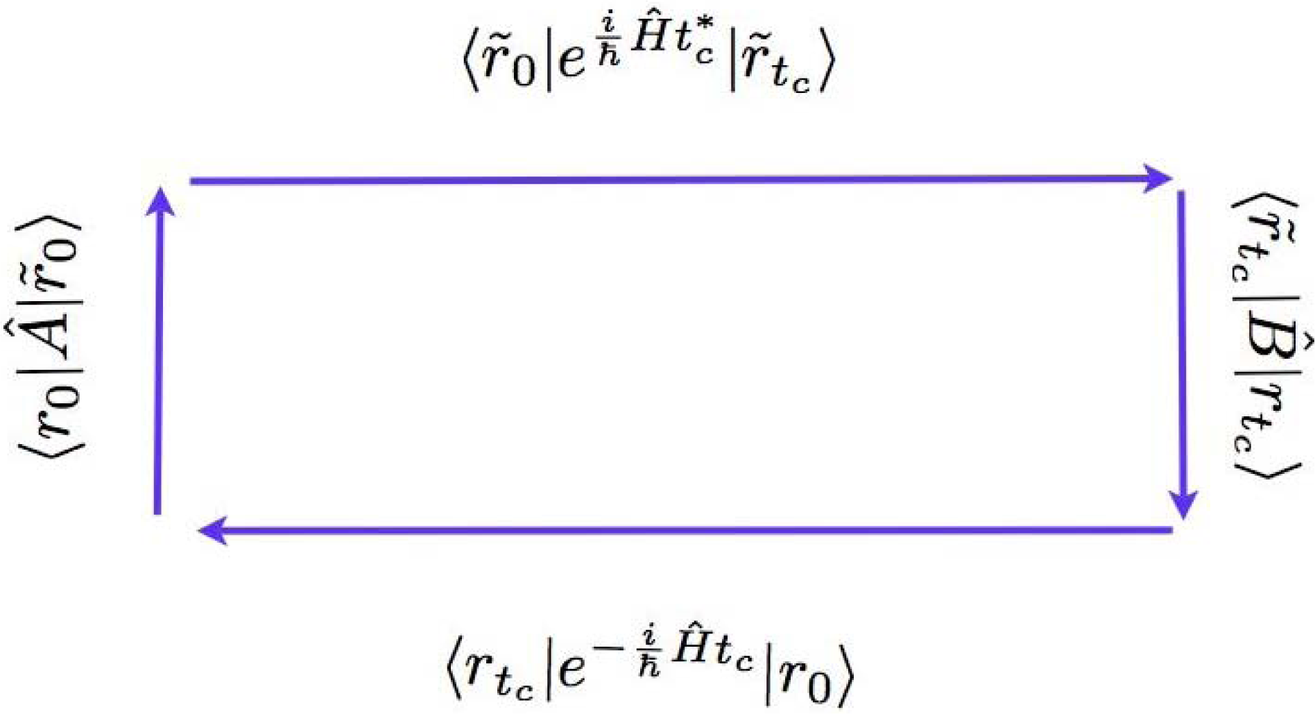
The structure of the integrand is represented in Figure 1 in which we show the sequence of matrix elements to be evaluated. Reading the figure from the bottom left corner up, we see the matrix element of operator Â, the backward complex time propagator (from r̃₀ to r̃_c), the matrix element of operator B̂ and, finally, the forward propagator that closes the circuit representing the trace operation. The difficult task is the evaluation of the propagators in complex time. To set the stage for the approximation we intend to perform, we use the time composition property to divide the two propagations into L segments of duration τ_c = t_c/L (τ_c need not be infinitesimal) and rewrite, for example:

$$\langle r_{t_c}\left|e^{-\frac{i}{\hslash }\hat{H}{t}_c}\right|r_0\rangle =\int d{r}_1\dots d{r}_{L-1}\prod _{J=0}^{L-1}\langle r_{J+1}\left|e^{-\frac{i}{\hslash }\hat{H}{\tau }_c}\right|r_J\rangle$$

(7)

with r_L = r_tc. Introducing an analogous expression for the backward propagator changes the scheme of the integrand as sketched in Figure 2, where each propagation lag (from J to J + 1) is indicated by the segment with arrows. We can now pair corresponding segments of propagation along the forward and backward paths, as indicated by the red frame in the figure, and define the product $K(r_{J+1},r_J;{\tilde{r}}_{J+1},{\tilde{r}}_J)=\langle {\tilde{r}}_{J+1}\left|e^{\frac{i}{\hslash }\hat{H}{\tau }_c^{*}}\right|{\tilde{r}}_J\rangle \langle r_{J+1}\left|e^{-\frac{i}{\hslash }\hat{H}{\tau }_c}\right|r_J\rangle$ to rewrite the symmetrized correlation function as:

$$\begin{array}{lll}{G}_{A,B}(t;\beta )\hfill & =\hfill & \frac{1}{Z}\int d{\tilde{r}}_{L}d{r}_L\langle {\tilde{r}}_L\left|\hat{B}\right|r_L\rangle \left\{\prod _{J=1}^{L-1}\int d{\tilde{r}}_{J}d{r}_{J}K\left(r_{J+1},r_J;{\tilde{r}}_{J+1},{\tilde{r}}_J\right)\right\}\hfill \\ \hfill & \times \hfill & \int d{r}_{0}d{\tilde{r}}_{0}K(r_1,r_0;{\tilde{r}}_1,{\tilde{r}}_0)\langle r_0\left|\hat{A}\right|{\tilde{r}}_0\rangle \hfill \end{array}$$

(8)

The expression above is an exact, incalculable, expression of the time correlation function. In the following, we will work on the generic K to obtain an approximate expression for it that has the key advantage of being analytically known as a product of functions calculable via an appropriate combination of Monte Carlo and molecular dynamics. To obtain this result, we first separate the real from the imaginary time part of the propagation by inserting one more resolution of the coordinate identity, thus:

$$\begin{array}{ll}K(r_{J+1},r_J;{\tilde{r}}_{J+1},{\tilde{r}}_J)\hfill & =\langle {\tilde{r}}_{J+1}\left|e^{\frac{i}{\hslash }\hat{H}{\tau }_c^{*}}\right|{\tilde{r}}_J\rangle \langle r_{J+1}\left|e^{-\frac{i}{\hslash }\hat{H}{\tau }_c}\right|r_J\rangle \hfill \\ \hfill & =\int d{\tilde{r}}_J^{\nu }d{r}_J^{\nu }\langle {\tilde{r}}_{J+1}\left|e^{\frac{i}{\hslash }\hat{H}{\tau }_t}\right|{\tilde{r}}_J^{\nu }\rangle \langle {\tilde{r}}_J^{\nu }\left|e^{-{\tau }_{\beta }\hat{H}}\right|{\tilde{r}}_J\rangle \langle r_{J+1}\left|e^{-\frac{i}{\hslash }\hat{H}{\tau }_t}\right|r_J^{\nu }\rangle \langle r_J^{\nu }\left|e^{-{\tau }_{\beta }\hat{H}}\right|r_J\rangle \hfill \end{array}$$

(9)

The two (thermal) propagators in the integrand above, associated with the inverse temperature, τ_β, can be expressed relatively easily in the path integral formalism as positive definite functions and interpreted, via the so-called classical isomorphism, as probability densities associated with systems of polymers. Well established techniques allow one to sample these densities. The real-time propagators, on the other hand, are prohibitive, even in path integral form. Feynman’s prescription requires, in fact, one to generate “all possible paths” connecting the initial and final point of the propagation, but, in contrast to the thermal case in which the probability density provides us with a sampling mechanism for the paths, no rule is given to determine them. Furthermore, even if we had a recipe for generating the paths, we would have to sum a (potentially infinite) set of phase factors, the exponential weighting each path. Capturing accurately the interference among these factors is essentially impossible (this is the well-known dynamical sign problem). As shown in detail in [30], progress can be made by deriving an approximate form for the product of the two real-time propagators in Equation (9). In analogy with the standard linearization methods mentioned in the Introduction, this is done most conveniently using a hybrid coordinate momenta representation of the propagators. The propagation time is divided into n intervals of length δ_t = τ_t/n, and appropriate resolutions of the identity are introduced to isolate matrix elements of the propagator for each short time interval. As usual, after a Trotter break up of the exponential of the Hamiltonian is performed, the (diagonal) exponential of the potential can be trivially evaluated. The matrix element of the kinetic energy part of the propagator, on the other hand, is easily evaluated by inserting a resolution of the identity in the momenta. Contrary to what is done in standard path integrals, however, the resulting generalized Gaussian integral in the momenta is not performed analytically, but left in the expression. This sequence of operations results in:

$$\langle {\tilde{r}}_{J+1}\left|e^{\frac{i}{\hslash }\hat{H}{\tau }_t}\right|{\tilde{r}}_J^{\nu }\rangle \langle r_{J+1}\left|e^{-\frac{i}{\hslash }\hat{H}{\tau }_t}\right|r_J^{\nu }\rangle \approx \int \prod _{l=1}^n\frac{d{\tilde{p}}_J^l}{2\pi \hslash }\prod _{l=1}^{n-1}d{\tilde{r}}_J^{\nu +l}{e}^{-\frac{i}{\hslash }S(\left\{\tilde{r},\tilde{p}\right\})}\int \prod _{l=1}^n\frac{d{p}_J^l}{2\pi \hslash }\prod _{l=1}^{n-1}d{r}_J^{\nu +l}{e}^{\frac{i}{\hslash }S(\left\{r,p\right\})}$$

(10)

where ({r, p}) indicates the full set of path variables and $S\left(\left\{r,p\right\}\right)={\sum }_{l=1}^n\left\{p_J^l\left(r_J^{(\nu +l)}-r_J^{(\nu +l-1)}\right)-\delta t\left[{\left(p_J^l\right)}^2/2m-V\left(r_J^{(\nu +l-1)}\right)\right]\right\}$ with analogous definitions for the tilde variables. The expression above becomes exact for n → ∞. At this stage, the forward and backward path integrals above are independent. Proceeding in analogy with standard linearization methods, we combine them by introducing the semi-sum and difference variables:

$$\begin{array}{ll}{\overline{r}}_J^{\nu +l}=\frac{r_J^{\nu +l}+{\tilde{r}}_J^{\nu +l}}{2}\hfill & {\overline{p}}_J^l=\frac{p_J^l+{\tilde{p}}_J^l}{2}\hfill \\ \Delta r_J^{\nu +l}=r_J^{\nu +l}-{\tilde{r}}_J^{\nu +l}\hfill & \Delta p_J^l=p_J^l-{\tilde{p}}_J^l\hfill \end{array}$$

(11)

with l = 0, …, n. In these variables, the difference of actions in Equation (10) is a linear function in $\Delta p_J^l$. Integrals over the difference momenta can then be performed analytically and result in a set of delta functions (this originates the last set of deltas in Equation (12) below). The dependence of the difference of the actions on $\Delta r_J^{(\nu +l)}$ is more complicated: they appear in an explicit, linear term, but also in the argument of the potentials. This dependence can also be linearized via the expansion $V\left({\overline{r}}_J^{(\nu +l)}+\Delta r_J^{(\nu +l)}/2\right)-V\left({\overline{r}}_J^{(\nu +l)}-\Delta r_J^{(\nu +l)}/2\right)=\nabla V\left({\overline{r}}_J^{(\nu +l)}\right)\Delta r_J^{(\nu +l)}+o\left[{\left(\Delta r_J^{(\nu +l)}\right)}^3\right]$. This is the key approximation that we perform. An appropriate rescaling of the variables shows that the approximation is equivalent to a second order expansion in ℏ of the phase, but a more precise analysis of its validity is required and under consideration (see, also, the discussion at the end of this section). Bearing this in mind, we observe that, once the expansion is performed, also the integrals on the $\Delta r_J^{(\nu +l)}$ variables can be analytically solved, producing a second set of delta functions. Thus:

$$\begin{array}{l}\langle {\overline{r}}_J^{\nu }-\frac{\Delta r_J^{\nu }}{2}\left|e^{\frac{i}{\hslash }\hat{H}{\tau }_t}\right|{\overline{r}}_{J+1}-\frac{\Delta r_{J+1}}{2}\rangle \langle {\overline{r}}_{J+1}+\frac{\Delta r_{J+1}}{2}\left|e^{-\frac{i}{\hslash }\hat{H}{\tau }_t}\right|{\overline{r}}_J^{\nu }+\frac{\Delta r_J^{\nu }}{2}\rangle \approx \\ \int d{\overline{r}}_J^{\nu +1}\dots d{\overline{r}}_J^{\nu +n-1}\int d{\overline{p}}_J^1\dots d{\overline{p}}_J^n{e}^{\frac{i}{\hslash }{\overline{p}}_J^n\Delta r_J^{(\nu +n)}}{e}^{-\frac{i}{\hslash }{\overline{p}}_J^1\Delta r_J^{\nu }}\\ \times \prod _{l=1}^{n-1}\delta \left[\left({\overline{p}}_J^{(l+1)}-{\overline{p}}_J^l\right)+{\delta }_t\nabla V({\overline{r}}_J^{(\nu +l)})\right]\prod _{l=1}^n\delta \left[\frac{{\overline{p}}_J^l}{m}{\delta }_t-({\overline{r}}_J^{(\nu +l)}-{\overline{r}}_J^{(\nu +l-1)})\right]\end{array}$$

(12)

The linearization approximation then has two crucial consequences: (1) by allowing the integration over the difference paths, it transforms the quantum expression of the correlation function, which, in the beginning, includes two propagators and, therefore, two paths, into a formula where only the semi-sum path appears, thus leading to a structure more similar to classical time correlations in which only one propagation is present; (2) (perhaps more importantly) it forces the semi-sum path to follow a, classical, Hamiltonian trajectory, as identified by the arguments of the delta functions.

The final step to obtain a suitable expression for Equation (9) does not introduce any further approximation. Let us consider again the product of the thermal propagators in the equation. As mentioned above, these can be written via standard coordinate path integrals. Once this is done, it is convenient to introduce also for these propagators semi-sum and difference path (this is important, in particular, to ensure that the common boundaries of the thermal and real-time propagations, $r_J^{\nu }$ and ${\tilde{r}}_J^{\nu }$, are represented coherently). In the semi-sum and difference variables, the product of the thermal propagators takes the form:

$$\begin{array}{l}\langle {\overline{r}}_J-\frac{\Delta r_J}{2}\left|e^{-\hat{H}{\tau }_{\beta }}\right|{\overline{r}}_J^{\nu }-\frac{\Delta r_J^{\nu }}{2}\rangle \langle {\overline{r}}_J^{\nu }\_\frac{\Delta r_J^{\nu }}{2}\left|e^{-\hat{H}{\tau }_{\beta }}\right|{\overline{r}}_J+\frac{\Delta r_J}{2}\rangle \approx {\left[\frac{m}{2\pi \hslash {\delta }_{\beta }}\right]}^{(\nu -1)}\\ \int d{\overline{r}}_J^1\dots d{\overline{r}}_J^{\nu -1}\int d\Delta r_J^1\dots d\Delta r_J^{\nu -1}{e}^{-{\delta }_{\beta }{\sum }_{\lambda =1}^{\nu }\left[V\left({\overline{r}}_J^{(\lambda -1)}+\Delta r_J^{(\lambda -1)}/2\right)+V\left({\overline{r}}_J^{(\lambda -1)}-\Delta r_J^{(\lambda -1)}/2\right)\right]}\\ \times e^{-\frac{{\sigma }_p^2}{2}{\sum }_{\lambda =1}^{\nu }{\left(\Delta r_J^{\lambda }+\Delta r_J^{(\lambda -1)}\right)}^2}{e}^{-\frac{1}{{\sigma }_r^2}{\sum }_{\lambda =1}^{\nu }{\left({\overline{r}}_J^{\lambda }-{\overline{r}}_J^{(\lambda -1)}\right)}^2}\end{array}$$

(13)

with ${\sigma }_p^2=m/2{\delta }_{\beta }\hslash$ and ${\sigma }_r^2=\hslash {\delta }_{\beta }/2m$. Substituting Equations (12) and (13) in Equation (9), it can be noted that the integral over Δr^ν is of a Gaussian form and can be performed analytically. Introducing the notation ${𝒳}_J=\left({\left\{{\overline{r}}_J^{\lambda }\right\}}_{\lambda =0,\dots \nu },{\left\{\Delta r_J^{\lambda }\right\}}_{\lambda =0,\dots \nu -1},{\left\{{\overline{r}}_J^{\nu +l}\right\}}_{l=1,\dots n-1},{\left\{{\overline{p}}_J^{\lambda }\right\}}_{l=l,\dots n}\right)$, after integration over Δr^ν, the linearized short time propagator can be written as:

$$K^l\left({\overline{r}}_{J+1},\Delta r_{J+1};{\overline{r}}_J,\Delta r_J\right)=\int d{𝒳}_J{e}^{\frac{i}{\hslash }{\overline{p}}_J^n\Delta r_{J+1}}\rho ({𝒳}_J,{\overline{r}}_{J+1})e^{-\frac{i}{\hslash }{\overline{p}}_J^1\Delta r_J^{(\nu -1)}}$$

(14)

with:

$$\begin{array}{ll}\rho ({𝒳}_J,{\overline{r}}_{J+1})\hfill & =\prod _{l=1}^{n-1}\delta \left[\left({\overline{p}}_J^{(l+1)}-{\overline{p}}_J^l\right)+{\delta }_t\nabla V({\overline{r}}_J^{(\nu +l)})\right]\prod _{l=1}^n\delta \left[\frac{{\overline{p}}_J^l}{m}{\delta }_t-({\overline{r}}_J^{(\nu +l)}-{\overline{r}}_J^{(\nu +l-1)})\right]\hfill \\ \hfill & \times e^{-{\delta }_{\beta }{\sum }_{\lambda =1}^{\nu }\left[V\left({\overline{r}}_J^{(\lambda -1)}+\Delta r_J^{(\lambda -1)}/2\right)+V\left({\overline{r}}_J^{(\lambda -1)}-\Delta r_J^{(\lambda -1)}/2\right)\right]}\hfill \\ \hfill & \times e^{-\frac{{\left({\overline{p}}_J^1\right)}^2}{2{\sigma }_p^2}}{e}^{-\frac{{\sigma }_p^2}{2}{\sum }_{\lambda =1}^{(\nu -1)}{\left(\Delta r_J^{\lambda }-\Delta r_J^{(\lambda -1)}\right)}^2}{e}^{-\frac{1}{{\sigma }_r^2}{\sum }_{\lambda =1}^{\nu }{\left({\overline{r}}_J^{\lambda }-{\overline{r}}_J^{(\lambda -1)}\right)}^2}\hfill \end{array}$$

(15)

(The Gaussian in ${\overline{p}}_J^1$, the first factor in the last line of the expression above, is the result of the integration over Δr^ν.) Substituting the approximate form of the propagator between complex time slices J and J + 1, we obtain for the symmetrized correlation function:

$$\begin{array}{ll}{G}_{A,B}^{(L)}(t,\beta )\hfill & =\frac{1}{Z}\int d\Delta r_{t_c}d{\overline{r}}_{t_c}\langle {\overline{r}}_{t_c}+\frac{\Delta r_{t_c}}{2}\left|\hat{B}\right|{\overline{r}}_{t_c}-\frac{\Delta r_{t_c}}{2}\rangle \hfill \\ \hfill & \times \prod _{J=1}^{L-1}\int d{𝒳}_J{e}^{\frac{i}{\hslash }{\overline{p}}_J^n\Delta r_{J+1}}\rho ({𝒳}_J,{\overline{r}}_{J+1})e^{-\frac{i}{\hslash }{\overline{p}}_J^1\Delta r_J^{(\nu -1)}}\hfill \\ \hfill & \times \int d{𝒳}_0{e}^{\frac{i}{\hslash }{\overline{p}}_0^n\Delta r_1}\rho ({𝒳}_0,{\overline{r}}_1)e^{-\frac{i}{\hslash }{\overline{p}}_0^1\Delta r_0^{(\nu -1)}}\langle {\overline{r}}_0+\frac{\Delta r_0}{2}\left|\hat{A}\right|{\overline{r}}_0-\frac{\Delta r_0}{2}\rangle \hfill \end{array}$$

(16)

The expression above is interesting. First of all, assuming that the linearization approximation of each short time propagator improves when the propagation time goes to zero, there is potential for systematic improvement with increasing L, and indeed, numerical tests [30] indicate that this is the case. However, the limit for large L, and, in particular, the validity of the expansion in the difference path at the intermediate times of the propagation, is delicate. In fact, while it can be argued that the matrix elements of operators  and B̂ (usually diagonal) force the forward and backward paths (the free and tilde variables in the upper panel of Figure 1) to start and end close to one another, and, therefore, that only small values of the difference among the paths will be relevant close to the initial and final time, truncating the expansion of the difference of the potentials along the whole pair of paths is considerably more delicate. This issue, and the nature of the dynamics when L → ∞, are currently under investigation. In the meantime, note that the ρ functions are positive definite, so that they can be used to define a probability density for sampling the overall path variables (i.e., the full set of {$𝒳$_J}_{J= 0,...,L−1} variables) as $\Pi =\frac{1}{\Omega }{\prod }_{J=0}^{L-1}\rho ({𝒳}_J,{\overline{r}}_{J+1})$, where Ω is the (unknown) normalization factor. The method to deal with this factor is illustrated in the next subsection for the case L = 1 and can be straightforwardly generalized to L > 1. The probability density, Π, corresponds to a stochastic process, which concatenates the thermal and time propagations within each short time propagator, K^l. The structure of the propagations in real and imaginary time is determined by the definition of ρ in Equation (15) and can be described as follows. For L = 1, there is only one real-time leg of duration τ_t = t, while the imaginary time propagation corresponds to an inverse temperature β/2 for both the semi-sum and difference variables. The upper panel of Figure 3 illustrates these propagations with a sketch. In the figure, the horizontal axis is time and the vertical axis temperature. The vertical plane represents the space of configurations associated with the thermal path integral for both the semi-sum and difference variables; the thermal beads are represented with the red circles. The harmonic interactions in the thermal paths are indicated with zigzagged lines connecting adjacent beads, while the interactions among the two paths due to the potential are drawn as dashed lines. Note that the difference variables path, on the left in the vertical plane in the figure, has one less bead than the semi-sum variables path, due to the integration carried out to isolate a Gaussian probability density for the initial momenta. The propagation in real time is drawn as the curve on the horizontal plane, which represents the phase space of the system. The red and golden circle at t = 0 represents the initial conditions for the time evolution: the initial coordinate coincides with the last bead of the thermal path in the semi-sum variables, while the initial momentum is sampled from the Gaussian mentioned before. A phase factor is associated with the initial point of the classical propagation. The exponent of this phase couples the initial momentum of the trajectory with the last bead of the thermal path in the difference variables. A phase factor is also associated with the final point of the classical propagation, where, for L = 1, the exponent couples the momentum at time t with the variable, Δr₁. The integrals over $\Delta r_0^{(\nu -1)}$ and Δr₁ in the expression for $G_{AB}^1(t;\beta )$ involve products of these phase factors with the matrix elements of operators  and B̂. The end-point integral reconstructs the Wigner transform of the operator, B̂. To see this, consider Equation (16). For L = 1, the second line of the equation is absent, and boundary conditions impose Δr₁ = Δr_tc (with similar relationships for the sum variables). With this notation, the integral over Δr_tc is recognizable as the Wigner transform of operator B̂. The structure of the sequence of imaginary and real-time propagation for generic values of L can be inferred from the lower part of Figure 3, where we show what happens for L = 2. In this case, there are two segments of classical dynamics, each of duration t/2, and two propagations of semi-sum and difference variables in imaginary time, taking the system from zero inverse temperature to β/4 and from β/4 to β/2, respectively. As before, the first segment of dynamics starts, with a Gaussian initial momentum, from the last bead of the semi-sum variable thermal path at t = 0. The end-point of this leg of propagation is the initial configuration for the semi-sum variable thermal path at t/2, and the second segment of dynamics has as initial conditions the final coordinate of the semi-sum variable thermal path and a new momentum sampled from a Gaussian. The variances of the Gaussians associated with the momentum sampling are doubled with respect to the case L = 1. The integrand now contains four phase factors coupling the momenta at the beginning and end of each classical dynamics segment with the values of the difference path variables at the end and at the beginning of each thermal slice, respectively. The phase factor that depends on $\Delta r_2{\overline{p}}_1^n$ (i.e., the phase factor computed at time t) can again be combined with the matrix element of operator B̂ to obtain the Wigner transform of this operator at the final time of the propagation, so that only three phases remain to contribute to the result. In general, $G_{AB}^{(L)}(t;\beta )$ involves L segments of classical propagation, each of duration t/L, interspersed with L pairs of thermal paths in the semi-sum and difference variables, each at an inverse temperature β/2L. The rules for connecting the coordinate and momenta at the initial and final time of the dynamics with the final and initial points of the thermal paths and for constructing the 2L − 1 phase factors contributing to the integrand (the phase factor at time t can always be absorbed in the Wigner transform of operator B̂) are completely analogous to the L = 2 case.

A Monte Carlo algorithm to sample Π for different values of L was illustrated in [30]. This Monte Carlo has several non-standard features, most notably the fact that the normalization of the probability density is unknown and that Π contains products of delta functions, i.e., singular distributions. These difficulties can be circumvented as detailed in [30]. The first one is tackled by recasting (without further approximations) Equation (16) in the form of a ratio of expected values. The second is addressed via an appropriate choice of the trial moves and acceptance probabilities. The most serious numerical difficulty, unfortunately, comes from the estimator of the observable. In fact, from Equation (16), it can be seen that, in addition to the matrix elements of the operators, the integrand contains a product of phase factors to be evaluated at the beginning and end of each real-time propagation segment. As mentioned above, the number of these phase factors for the “order L” approximation of the symmetrized correlation function is 2L − 1, and their presence rapidly hinders the convergence of the calculation. Furthermore, for a system of n particles in three dimensions, the phases take the (generic) form $e^{\pm \frac{1}{\hslash }\mathbf{p}\cdot \Delta \mathbf{r}}$, where p and Δr are 3n-dimensional vectors. The number of phase factors thus scales linearly with the number of degrees of freedom, so that, even for small values of L, convergence is problematic. The numerical tests performed so far on simple model systems confirm both the interest and the difficulties of Equation (16). In [30], we computed position autocorrelation functions for a set of one-dimensional systems (e.g., quartic potential) at temperatures low enough to ensure that the system was in the quantum regime. We observed that increasing the number of complex time slices did systematically improve the length of time for which we were able to get accurate results. However, the numerical effort to go beyond L = 3, though not exponential in time, became essentially prohibitive, even for these simple systems. To indicate possible means to reduce the numerical effort involved in these calculations, we now discuss a recent development of the method developed to address the problem of the phase in the simplest case, L = 1, in which it presents itself. We then illustrate how to formally extend this development, which, in its simplest form, has been successfully applied to realistic models of condensed phase systems, to the case L > 1.

3. L = 1: Fully Linearized Approximation

The expression for the L = 1 approximation of the symmetrized correlation function is given by (see Equation (16)):

$$\begin{array}{ll}{G}_{A,B}^{(1)}(t;\beta )\hfill & =\frac{1}{Z}\int d\Delta r_{t_c}d{\overline{r}}_{t_c}\int d{𝒳}_0\langle {\overline{r}}_{t_c}+\frac{\Delta r_{t_c}}{2}\left|\hat{B}\right|{\overline{r}}_{t_c}-\frac{\Delta r_{t_c}}{2}\rangle e^{\frac{i}{\hslash }{\overline{p}}_0^n\Delta r_{t_c}}\hfill \\ \hfill & \times \rho ({𝒳}_0,{\overline{r}}_{t_c})e^{-\frac{i}{\hslash }{\overline{p}}_0^1\Delta r_0^{(\nu -1)}}\langle {\overline{r}}_0+\frac{\Delta r_0}{2}\left|\hat{A}\right|{\overline{r}}_0-\frac{\Delta r_0}{2}\rangle \hfill \end{array}$$

(17)

We are now going to simplify the expression above using four steps: (1) observe that the integral over Δr_tc in the first line of the equation above defines the Wigner transform of operator B̂ (see, also, the definition below Equation (4)); (2) note that the product of δ functions in the definition of ρ (Equation (15)) forces (r̃_tc, ${\overline{p}}_{t_c}^n$) to be endpoints of a classical trajectory of length t starting at ( ${\overline{r}}_0^{\nu }$, ${\overline{p}}_0^1$), so that, after integration over r̄^(ν+l) (l = 1, ..., n − 1) and p̄^l (l = 1, ..., n), (r̄_tc, ${\overline{p}}_{t_c}^n$) = (r_t, p_t) (where (r_t, p_t) denote the classically evolved variables); (3) choose, for the sake of simplicity, to specialize the discussion to an operator, Â, which is diagonal in the coordinate representation (the case of generic operators is considered in the Appendix of [39]). This choice, producing a δ(Δr₀) in the evaluation of the matrix elements, allows one to integrate also over Δr₀. The surviving variables (i.e., the semi-sum and difference variables of the thermal path integral and the initial momentum of the classical trajectory) will be indicated collectively as Γ = {p¹, r⁰, …, r^ν, Δr¹, …, Δr^ν−1}; (4) simplify the notation by dropping the bar from the semi-sum variables and the subscript, which identifies the J = 0 propagation segment in Equation (16), since only one segment is now present. Once these operations are performed, the correlation function can be written as:

$$G_{A,B}^{(1)}(t;\beta )=\frac{\hat{Q}}{Z}\int d\Gamma B_w\left(r_t,p_t\right)P(\Gamma )e^{-\frac{i}{\hslash }{p}^1\Delta r^{(\nu -1)}}A(r^0)$$

(18)

with

$$\begin{array}{ll}P(\Gamma )\hfill & =\frac{1}{\hat{Q}}{e}^{-\frac{{\left(p^1\right)}^2}{2{\sigma }_p^2}}{e}^{-2{\delta }_{\beta }V(r^0)}{e}^{-\frac{1}{2{\sigma }_r^2}{\sum }_{\lambda =1}^{\nu }{\left(r^{\lambda }-r^{\lambda -1}\right)}^2}{e}^{-\frac{{\sigma }_p^2}{2}{\sum }_{\lambda =2}^{\nu -1}{\left(\Delta r^{\lambda }-\Delta r^{\lambda -1}\right)}^2}{e}^{-\frac{{\sigma }_p^2}{2}{\left(\Delta r^1\right)}^2}\hfill \\ \hfill & \times e^{-{\delta }_{\beta }{\sum }_{\lambda =2}^{\nu }\left[V\left(r^{(\lambda -1)}+\frac{\Delta r^{(\lambda -1)}}{2}\right)+V\left(r^{(\lambda -1)}-\frac{\Delta r^{(\lambda -1)}}{2}\right)\right]}\hfill \end{array}$$

(19)

and Q̂ the normalization of P(Γ). Note that the expression above for the probability is quite standard, being an explicit function of the semi-sum and difference variables, which can be sampled via Monte Carlo, multiplied by a Gaussian term for the momenta. As mentioned in the previous section, the ratio of the normalization over the partition function, which appears in Equation (18), is, in general, not known, and we estimate it via the autocorrelation of the identity, $G_{I,I}^{(1)}=1=\frac{\hat{Q}}{Z}\int d\Gamma P(\Gamma )e^{-\frac{i}{\hslash }{p}^1\Delta r^{(\nu -1)}}$ Using this approach, the L = 1 estimator of the correlation function is given by the following ratio of expectation values over P(Γ):

$$G_{A,B}^{(1)}(t;\beta )=\frac{{\langle B_w(r_t,p_t)e^{-\frac{i}{\hslash }{p}^1\Delta r(\nu -1)}A(r^0)\rangle }_P}{{\langle e^{-\frac{i}{\hslash }{p}^1\Delta r(\nu -1)}\rangle }_P}$$

(20)

As anticipated, both in the numerator and denominator of this expression, a phase factor appears, which, for high dimensional systems, hinders an efficient convergence of the calculation. To alleviate this problem, we proposed a method, described in detail in [39], which starts by obtaining an alternative expression for $G_{A,B}^{(1)}$. As will be shown in the following, the new expression does not introduce further (analytical) approximations, but it has the advantage of eliminating the phase factor from the observable. Let us consider in more detail the structure of the probability, P(Λ). This probability is given by the product of a Gaussian for the momenta, ${\rho }_G(p)\propto e^{-\frac{p^2}{2{\sigma }_p^2}}$ (note that, with respect to Equation (19), we dropped the superscript, 1, on the momenta to simplify the notation), times a joint probability function for the semi-sum and difference thermal variables to be indicated in the following as ρ̃(r, Δr), where we have introduced the notation r = {r⁰, …, r^ν} and Δr = {Δr¹, …, Δr^(ν−1)}. This joint probability (whose form can be inferred from Equation (19) by taking out the momentum Gaussian) is most conveniently expressed as:

$$\tilde{\rho }=(\mathbf{r},\Delta \mathbf{r})={\rho }_c(\Delta \mathbf{r}|\mathbf{r}){\rho }_m(\mathbf{r})$$

(21)

where:

$$\begin{array}{ll}{\rho }_m(\mathbf{r})\hfill & =\frac{1}{\hat{Q}}{e}^{-2{\delta }_{\beta }V(r^0)}{e}^{-\frac{1}{2{\sigma }_r^2}{\sum }_{\lambda =1}^{\nu }{\left(r^{\lambda }-r^{\lambda -1}\right)}^2}\int d\Delta \mathbf{r}{e}^{-\frac{{\sigma }_p^2}{2}{\sum }_{\lambda =2}^{\nu -1}{\left(\Delta r^{\lambda }-\Delta r^{\lambda -1}\right)}^2}{e}^{-\frac{{\sigma }_p^2}{2}{\left(\Delta r^1\right)}^2}\hfill \\ \hfill & =e^{-{\delta }_{\beta }{\sum }_{\lambda =2}^{\nu }\left[V\left(r^{(\lambda -1)}+\frac{\Delta r^{\lambda -1}}{2}\right)+V\left(r^{(\lambda -1)}-\frac{\Delta r^{\lambda -1}}{2}\right)\right]}\hfill \end{array}$$

(22)

is the marginal probability for the semi-sum variables and ρ_c(Δr|r) ≡ ρ̃(r, Δr)/ρ_m(r) is the conditional probability for the difference variables given the semi-sum variables. This rewriting of the probability density is convenient because the phase factors in Equation (20) depend only on the momenta and difference variables. We can use this observation to define:

$$F(p,\mathbf{r})={\int d\Delta \mathbf{r}e}^{-\frac{i}{\hslash }p\Delta r^{(\nu -1)}}{\rho }_c(\Delta \mathbf{r}|\mathbf{r})$$

(23)

which is the average of the phase with respect to the conditional probability density, and investigate the properties of this function to see if we can use them to improve the convergence of our calculations. To that end, note that F is also, by definition, the cumulant generating function of the variable Δr^(ν−1) with respect to the conditional probability, ρ_c(see, for example, [40,41] for previous use of cumulants in this field). This means that the coefficients of the Taylor series expansion (with respect to −ip/ℏ):

$$\text{ln}F(p,\mathbf{r})=\sum _{n=1}^{\infty }\frac{{\left(-ip/\hslash \right)}^n}{n!}{\langle {\left(\Delta r^{(\nu -1)}\right)}^n\rangle }_{{\rho }_c(\Delta \mathbf{r}|\mathbf{r})}^c$$

(24)

(these coefficients are indicated above as ${\langle {\left(\Delta r^{(\nu -1)}\right)}^n\rangle }_{{\rho }_c(\Delta \mathbf{r}|\mathbf{r})}^c$) are the cumulant moments of Δr^(ν−1). Importantly, the conditional probability density is an even function of the difference variables, implying that only even order terms in the series above are non-zero and that the series corresponds to a real function that we will denote in the following with E(p, r). We can then express the average of the phase as:

$$F(p,\mathbf{r})=e^{-E(p,\mathbf{r})}$$

(25)

i.e., a positive definite function of the momenta and the semi-sum variables. We now use the function above to define a new probability density:

$$𝒫(p,\mathbf{r})=\frac{{\rho }_g(p)e^{-E(p,\mathbf{r})}{\rho }_m(\mathbf{r})}{\int dpd\mathbf{r}{\rho }_g(p)e^{-E(p,\mathbf{r})}{\rho }_m(\mathbf{r})}$$

(26)

and note that, by direct substitution of this definition in the (explicit) expression of Equation (20), we obtain:

$$G_{A,B}^{(1)}(t;\beta )={\langle B_w(r_t,p_t)A(r^0)\rangle }_{𝒫}$$

(27)

The key advantage of the expression above is that the observable does not contain phase factors anymore and is, therefore, well suited for a Monte Carlo estimate. Sampling the distribution, $𝒫$, however, is non-trivial, since this probability density contains two factors, e^−E(p,r) and ρ_m(r), that do not have an explicit analytic form, but, for each value of r and p, can only be estimated numerically. The numerical estimate of E(r, p), in particular, requires one to truncate the cumulant series at a given order. The convergence of the calculation with respect to truncation of the series can always be checked numerically, and, although the cost scales up where terms of higher order are included, it does not present any particular difficulty. (In all calculations performed so far, a second order cumulant expansion proved sufficient.) In the following subsection, we briefly describe how to combine two schemes, known as the Kennedy and Penalty methods, for Monte Carlo sampling of noisy probability densities and obtain $G_{A,B}^{(1)}(t;\beta )$. Our goal is to highlight the main differences among these schemes and standard Monte Carlo and to indicate where the algorithm is most affected by them. A detailed description of the algorithm can be found in [38,39].

3.1. Noisy Monte Carlo Algorithm

To simplify the discussion, we introduce some notation. Let us indicate the coordinate-dependent Gaussian terms in Equation (19) as:

$$\begin{array}{l}{e}^{-\frac{1}{2{\sigma }_r^2}{\sum }_{\lambda =1}^{\nu }{\left(r^{\lambda }-r^{(\lambda -1)}\right)}^2}=e^{-{\mathbf{V}}_r(\mathbf{r})}\\ e^{-\frac{{\sigma }_p^2}{2}{\sum }_{\lambda =1}^{\nu -1}{\left(\Delta r^{\lambda }-\Delta r^{(\lambda -1)}\right)}^2}=e^{-{\mathbf{V}}_{\Delta }(\Delta \mathbf{r})}\end{array}$$

(28)

(above Δr⁰ = 0) and write the potential term as:

$$\begin{array}{l}{e}^{-{\delta }_{\beta }{\sum }_{\lambda =2}^{\nu }\left[\mathbf{V}(r^{(\lambda -1)}+{\frac{\Delta r}{2}}^{(\lambda -1)})+\mathbf{V}(r^{(\lambda -1)}-{\frac{\Delta r}{2}}^{(\lambda -1)})\right]}{e}^{-2{\delta }_{\beta }\mathbf{V}(r^0)}\\ =e^{-{\delta }_{\beta }\overline{\mathbf{V}}(\mathbf{r},\Delta \mathbf{r})}\end{array}$$

(29)

We also rewrite the marginal probability, ρ_m(r), defined in Equation (22), isolating the terms that do not depend on Δr and have an explicit analytic expression, thus:

$$\begin{array}{lll}{\rho }_m(\mathbf{r})\hfill & =\hfill & \int d\Delta \mathbf{r}\tilde{\rho }(\mathbf{r},\Delta \mathbf{r})=\frac{1}{Q}{e}^{-{\mathbf{V}}_r(\mathbf{r})}\int d\Delta \mathbf{r}\hspace{0.17em}\hspace{0.17em}{e}^{-{\delta }_{\beta }\overline{\mathbf{V}}(\mathbf{r},\Delta \mathbf{r})}{e}^{-{\mathbf{V}}_{\Delta }(\Delta \mathbf{r})}\hfill \\ \hfill & =\hfill & \frac{1}{Q}{e}^{-{\mathbf{V}}_r(\mathbf{r})}{\rho }_m^{\text{'}}(\mathbf{r})\hfill \end{array}$$

(30)

With the definitions above, $𝒫$(p, r) takes the form:

$$𝒫(p,\mathbf{r})=\frac{1}{𝒬}{\rho }_G(p)e^{-E(\mathbf{r},p)}{e}^{-{\mathbf{V}}_r(\mathbf{r})}{{\rho }^{\prime }}_m(\mathbf{r})$$

(31)

where $𝒬$ is the normalization. The scheme that we use to perform the sampling is based on earlier work by Ceperley [42] and Kennedy [43]. Adapting their ideas to our case, we will introduce a Monte Carlo algorithm in which the definition of the probability to generate a new state of the system by changing either the coordinates or the momenta of the particle (unlike what happens in classical canonical densities, in our probability, the variables, p and r, are not independent (with the momenta Gaussian and then integrable) and must be treated numerically) and/or to accept this new state is modified to guarantee that detailed balance is satisfied also when ${{\rho }^{\prime }}_m(\mathbf{r})$ and E(r, p) are estimated with significant noise. Both the Ceperley and Kennedy scheme require the introduction of appropriate numerical estimators of the unknown functions that will be indicated with calligraphic fonts.

The Monte Carlo scheme to sample Equation (31) is constructed as follows. Choose, with probability 1/2, if the move will involve r or p.

(1) A move on p has been selected:

choose a new momentum according to p′ = p + δp, where δp is a uniform random number centered on zero (the magnitude of the displacement is chosen so as to optimize the acceptance). Taking into account that the r variables are not being updated, detailed balance for this trial move takes the form:

$${\rho }_G(p)e^{-E(\mathbf{r},p)}{A}^p(p\to p^{\prime })={\rho }_G(p^{\prime })e^{-E(\mathbf{r},p^{\prime })}{A}^p(p^{\prime }\to p)$$

(32)

where A^p(p → p′) is the acceptance probability. The detailed balance relationship above has the same form as the one discussed by Ceperly et al. within the penalty method [42], a generalized Monte Carlo for sampling a density given by the exponential of a function, in our case E(., .), known with statistical errors. According to the penalty method, if a numerical estimate, Δ$ℰ$_p(p′, p; r), of the difference E(r, p′)−E(r, p) has been obtained (for example, by averaging N_s values of a specific estimator) and an estimate of its variance, ${\chi }_p^2$, is also known, detailed balance can be satisfied by defining the acceptance as:

$$A^p(p\to p^{\prime })=\text{min}\left[1,\frac{{\rho }_G(p^{\prime })}{{\rho }_G(p)}{e}^{-\Delta {ℰ}_p(p^{\prime };p;\mathbf{r})-u_{{\chi }_p^2}}\right]$$

(33)

where:

$$u_{{\chi }_p^2}=\frac{{\chi }_p^2}{2}+\frac{{\chi }_p^4}{4(N_s+1)}+\dots$$

(34)

The expression for the acceptance probability differs from the standard Metropolis prescription for the presence of $u_{{\chi }_p^2}$ and is valid when ${\chi }_p^2/n<1/4$ [42]. In the limit of an infinitely precise estimate of the difference, $u_{{\chi }_p^2}\to 0$ and the standard criterion is recovered; when non-zero, this function corrects, on average, for the effect of the noise.

(2) A move on r has been selected:

in this case, indicating with T^r(r → r′) and A^r(r → r′) the probability to generate and accept a new configuration, respectively, detailed balance is expressed, after simplifying ρ_G(p), as:

$$\begin{array}{l}{e}^{-E(\mathbf{r},p)}{e}^{-{\mathbf{V}}_r(\mathbf{r})}{{\rho }^{\prime }}_m(r)T^r(\mathbf{r}\to {\mathbf{r}}^{\prime })A^r(\mathbf{r}\to {\mathbf{r}}^{\prime })=\\ e^{-E({\mathbf{r}}^{\prime },p)}{e}^{-{\mathbf{V}}_r({\mathbf{r}}^{\prime })}{{\rho }^{\prime }}_m({\mathbf{r}}^{\prime })T^r({\mathbf{r}}^{\prime }\to \mathbf{r})A^r({\mathbf{r}}^{\prime }\to \mathbf{r})\end{array}$$

(35)

The structure of this relationship is analogous to the one considered by Kennedy et al. [43], who adapted Monte Carlo sampling to probability densities given by an exponential term times a “noisy” (positive definite) function. They showed that detailed balance is satisfied if states are generated according to the probability:

$$T^r(\mathbf{r}\to {\mathbf{r}}^{\prime })\propto e^{-E({\mathbf{r}}^{\prime },p)}{e}^{-{\mathbf{V}}_r({\mathbf{r}}^{\prime })}$$

(36)

(a method to sample T^r(r → r′) is described after the next equation) and accepted with probability:

$$A^r(\mathbf{r}\to {\mathbf{r}}^{\prime })=\{\begin{array}{ll}c𝒰(\mathbf{r}\to {\mathbf{r}}^{\prime })\hfill & \text{if}\hspace{0.17em}{e}^{-{\delta }_{\beta }\mathbf{V}(\mathbf{r},0)}>e^{-{\delta }_{\beta }\mathbf{V}({\mathbf{r}}^{\prime },0)}\hfill \\ c\hfill & \text{if}\hspace{0.17em}{e}^{-{\delta }_{\beta }\mathbf{V}(\mathbf{r},0)}\le e^{-{\delta }_{\beta }\mathbf{V}({\mathbf{r}}^{\prime },0)}\hfill \end{array}$$

(37)

Above, $𝒰$(r → r′) is an unbiased estimator of the ratio, ${{\rho }^{\prime }}_m({\mathbf{r}}^{\prime })/{{\rho }^{\prime }}_m(\mathbf{r})$, and c < 1 is a constant that ensures A^r(r → r′) ∈ [0, 1] (for details on the meaning and choice of c, see [43] and the discussion on page 8 of [39]). The conditions on the exponential of the potential enforce an ordering criterion on the states, whose optimal choice depends on the problem (here, we used the one adopted in our previous work [39]). In the usual implementation of the Kennedy method, the exponential part of the probability density is assumed to be known analytically, and the states are generated via a standard Monte Carlo method. In our case, the situation is more complicated, since e^−E(r′,p) is only known with noise. To solve this problem, we employ the penalty method to obtain configurations distributed according to Equation (36). These configurations are generated using a Monte Carlo with transition probability t(r → r′) ∝ e^−V_r(r′) and acceptance probability $a(r\to r^{\prime })=\text{min}[1,\text{exp}\hspace{0.17em}(-\Delta {ℰ}_r({\mathbf{r}}^{\prime },\mathbf{r};p)-u_{{\chi }_r^2})]$ where Δ$ℰ$_r(r′,r; p) is an unbiased estimator of E(r′, p) − E(r, p), and $u_{{\chi }_r^2}$ is defined in analogy with Equation (34).

This concludes the description of our Monte Carlo moves. The practical implementation of this algorithm requires the definition of the numerical estimators, $𝒰$(r → r′), Δ$ℰ$_p(p′, p; r) and Δ$ℰ$_r(r′, r; p). While this is an important technical point, it only involves a set of calculations, each performed via an auxiliary Monte Carlo move, that are quite standard. To provide a typical example, we consider one of the estimators referring the reader to [39] for a detailed description of the others. Let us then consider $𝒰$(r → r′). This quantity, necessary in the Kennedy acceptance test, see Equation (37), is obtained by writing the ratio of the marginal probabilities as:

$$\begin{array}{l}\frac{{{\rho }^{\prime }}_m({\mathbf{r}}^{\prime })}{{{\rho }^{\prime }}_m(\mathbf{r})}=\frac{\int d\Delta \mathbf{r}\hspace{0.17em}{e}^{-{\mathbf{V}}_{\Delta }(\Delta \mathbf{r})}{e}^{-{\delta }_{\beta }\overline{\mathbf{V}}({\mathbf{r}}^{\prime },\Delta \mathbf{r})}}{\int d\Delta \mathbf{r}\hspace{0.17em}{e}^{-{\mathbf{V}}_{\Delta }(\Delta \mathbf{r})}{e}^{-{\delta }_{\beta }\overline{\mathbf{V}}(\mathbf{r},\Delta \mathbf{r})}}\\ =\frac{\int d\Delta \mathbf{r}\hspace{0.17em}{e}^{-{\mathbf{V}}_{\Delta }(\Delta \mathbf{r})}{e}^{-{\delta }_{\beta }\overline{\mathbf{V}}(\mathbf{r},\Delta \mathbf{r})}{e}^{-{\delta }_{\beta }\left[\overline{\mathbf{V}}({\mathbf{r}}^{\prime },\Delta \mathbf{r})-\overline{\mathbf{V}}(\mathbf{r},\Delta \mathbf{r})\right]}}{\int d\Delta \mathbf{r}\hspace{0.17em}{e}^{-{\mathbf{V}}_{\Delta }(\Delta \mathbf{r})}{e}^{-{\delta }_{\beta }\overline{\mathbf{V}}(\mathbf{r},\Delta \mathbf{r})}}\\ ={\langle e^{-{\delta }_{\beta }\left[\overline{\mathbf{V}}\left({\mathbf{r}}^{\mathbf{\prime }},\Delta \mathbf{r}\right)-\overline{\mathbf{V}}\left(\mathbf{r},\Delta \mathbf{r}\right)\right]}\rangle }_{{\rho }_c\left(\Delta \mathbf{r}|\mathbf{r}\right)}\end{array}$$

(38)

whose unbiased estimator is:

$$𝒰(\mathbf{r}\to {\mathbf{r}}^{\prime })=\frac{1}{N_a}\sum _{i=1}^{N_a}{e}^{-{\delta }_{\beta }\left[\overline{\mathbf{V}}({\mathbf{r}}^{\prime },\Delta {\mathbf{r}}_i)-\overline{\mathbf{V}}(\mathbf{r},\Delta {\mathbf{r}}_i)\right]}$$

(39)

where {Δr_i} are a sample distributed according to ρ_c(Δr|r). This sample is obtained via an auxiliary (standard) Monte Carlo calculation over the conditional probability, ρ_c(Δr|r), in which new configurations are generated according to T (Δr → Δr′) ∝ exp[−V_Δ(Δr′)] (To do this, we use the staging method [44], which allows one to sample exactly a probability density containing Gaussian-like distributions, see Equation (28)), and moves are accepted or rejected based on A(Δr → Δr′) = min {1, exp[−δ_β(V̄ (r, Δr′) − V̄ (r, Δr)]}. As can be seen from the expression above, calculating the estimator requires N_a steps in the auxiliary Monte Carlo calculation. A similar situation arises when the other estimators introduced above are considered, so that the total number of Monte Carlo moves in our scheme is given by N_t = N_m × N_a, where we indicated with N_m the number of moves in the “main” Monte Carlo cycle (i.e., each choice of a move on r or p) and with N_a the number of auxiliary Monte Carlo steps per “main” move.

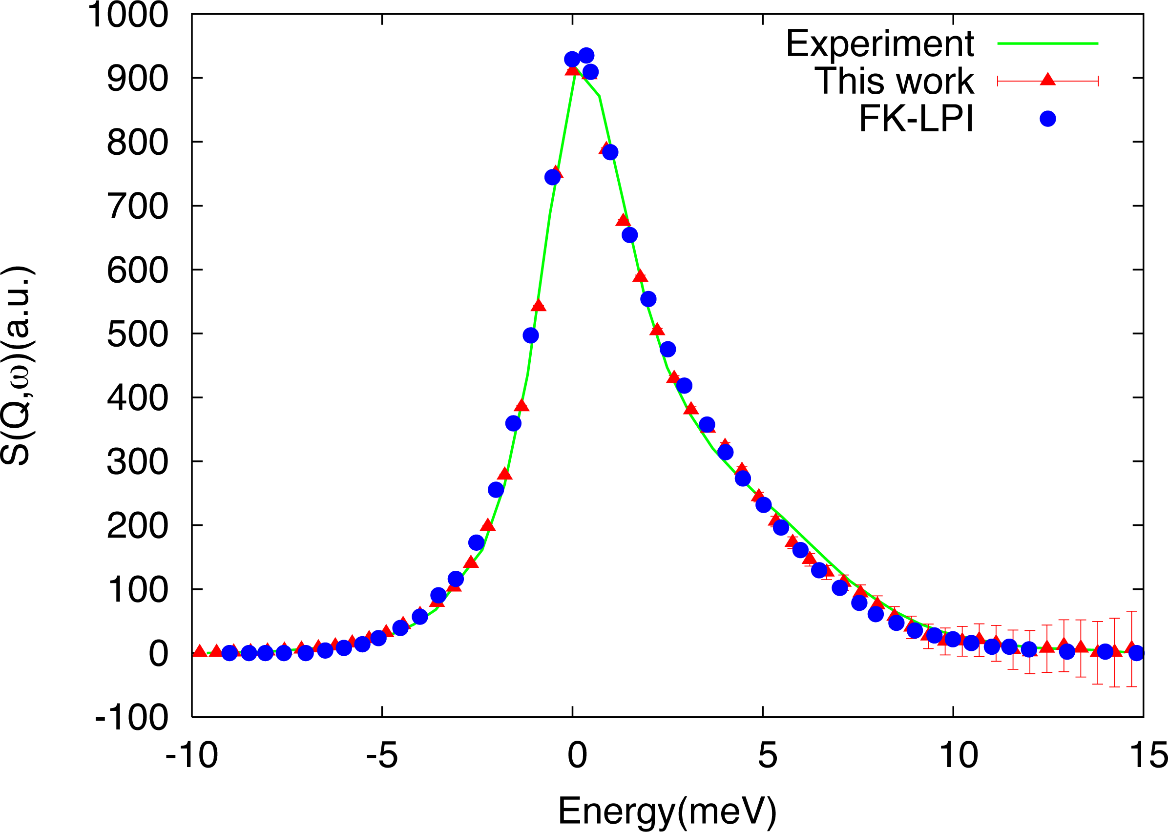
The computational overhead introduced by the auxiliary Monte Carlo calculation increases the cost of our calculation, but it is very small compared to the number of moves necessary to converge the estimate of Equation (20). The algorithm just described is, in fact, efficient enough to make possible calculations on realistic condensed phase systems with relatively little numerical effort. In particular, the algorithm was used to compute the dynamic structure factor of a model of liquid neon composed of 64 atoms [38]. Details of the calculation can be found in [38]. Here, we show, in Figure 4, our results (red triangles with error bars in the figure) and compare them with experiments (green curve) and the results of a calculation (with the same empirical potential and simulation parameters) performed by Poulsen et al. [45] using the linearized approximation for quantum time correlation functions described in the Introduction (see Equation (4) and the discussion above it).

The results show a rather pronounced asymmetry around zero, due to detailed balance, that indicates the presence of relevant quantum effects in the system. The agreement between our calculations and experiments is very good, as it is the agreement with the standard linearized calculation by Poulsen (a state-of-the-art reference in the field). The numerical cost of the two calculations is very similar (about a million Monte Carlo steps in total for initial condition sampling), showing that the auxiliary steps, due to the noisy distributions in our approach, are essentially irrelevant. Indeed, other tests indicate that, depending on the system, the overall cost of our method can be less than that of alternative schemes with comparable or better accuracy. The approach described in this section, for example, has also been used to obtain the infrared spectra of simple models of molecules in the gas phase [46]. Although these systems are quite small, the calculations that we performed are known to pose a considerable challenge to alternative, less rigorous methods, such as Centroid Molecular Dynamics [47] and Ring Polymer Molecular Dynamics [48], which fail to capture the spectra and/or introduce spurious features. In contrast, even though obtaining the exact intensities is quite expensive, our method proved remarkably effective in identifying the positions of the peaks, which could be obtained with only about one hundred Monte Carlo moves.

3.2. L > 1

In this subsection, we present a new development of the approach summarized above that extends the use of cumulants to pre-average the phase factors in the expression of the symmetrized correlation function to the case L > 1 (This possibility came out in discussions with M. Monteferrante.). For simplicity of notation, in this subsection, we describe how this can be done for L = 2, but the steps that we shall use can be generalized to a larger number of segments. In the following, we report the formal result, while the construction and test of an algorithm that generalizes the noisy Monte Carlo scheme described in the previous section will be the object of future work. Let us begin by rewriting the L = 2 approximation of the symmetrized correlation function, for diagonal Â, as follows (see Equations (16) and (20) for structure and notation):

$$G_{A,B}^{(2)}(t;\beta )=\frac{\int d{\Gamma }_{1}d{\Gamma }_0{B}_w(r_t^{(2)},p_t^{(2)})\left[e^{-\frac{i}{\hslash }{p}_1^1\Delta r_1^{(\nu -1)}}P({\Gamma }_1;r_0^n)e^{\frac{i}{\hslash }{p}_0^n\Delta r_1}\right]\hspace{0.17em}\hspace{0.17em}\left[e^{-\frac{i}{\hslash }{p}_0^1\Delta r_0^{(\nu -1)}}P({\Gamma }_0)\right]A(r_0)}{\int d{\Gamma }_{1}d{\Gamma }_0\left[e^{-\frac{i}{\hslash }{p}_1^1\Delta r_1^{(\nu -1)}}P({\Gamma }_1;r_0^n)e^{\frac{i}{\hslash }{p}_0^n\Delta r_1}\right]\hspace{0.17em}\hspace{0.17em}\left[e^{-\frac{i}{\hslash }{p}_0^1\Delta r^{(\nu -1)}}P({\Gamma }_0)\right]}$$

(40)

In the equation above, ( $r_t^{(2)},p_t^{(2)}$) is the endpoint of the propagation obtained by combining the two segments of classical dynamics described in the lower panel of Figure 3; ${\Gamma }_0=\left\{p_0^1,r_0^0,\dots r_0^{\nu },\hspace{0.17em}\Delta r_0^1,\dots ,\Delta r_0^{(\nu -1)}\right\}$ and ${\Gamma }_1=\left\{p_1^1,r_1^1,\dots r_1^{\nu },\hspace{0.17em}\Delta r_1^0,\dots ,\Delta r_1^{(\nu -1)}\right\}$ indicate the variables associated with the first and second set of thermal path integrals, respectively (the first set does not include $\Delta r_0^0$, since this variable can be integrated over for diagonal Â, and the second does not include $r_1^0\equiv \Delta r_0^n$, since this is the endpoint of the, deterministic, classical propagation from zero to t/2 in Figure 3). P(Γ₀) was defined in the previous section (see Equation (19)), and:

$$P({\Gamma }_1;r_0^n)={\rho }_G(p_1^1){\rho }_m({\mathbf{r}}_1;r_0^n){\rho }_c(\Delta {\mathbf{r}}_1|{\mathbf{r}}_1)$$

(41)

where ${\mathbf{r}}_1=\left\{r_1^1,\dots ,r_1^{\nu }\right\}$ and $\Delta {\mathbf{r}}_1=\left\{\Delta r_1^0,\dots ,\Delta r_1^{(\nu -1)}\right\}$. The Gaussian probability for the momenta, ${\rho }_G(p_1^1)$, and the marginal, ${\rho }_m({\mathbf{r}}_1;r_0^n)$, and conditional, ρ_c(Δr₁|r₁), probabilities are defined in analogy with the expressions introduced in Section 3, with the caveat that for J = 1 (and, in general, for J > 0), the sum involving the potentials in the second line of Equation (22) runs from one to ν − 1. In the marginal probability, we have also indicated the (parametric) dependence of the density on $r_0^n$, i.e., the endpoint of the classical propagation of the first segment, which corresponds, due to the boundary condition mentioned above, to the first bead of the concatenated semi-sum thermal path. The square brackets in Equation (40) isolate the terms that play the most significant role in the following. The first bracket from the left (corresponding to the J = 0 term in the approximation of the correlation function) is the same as the one we encountered in the previous subsection, while the second shows the general structure of the terms involving the phase factors for J > 0. As summarized when discussing Figure 3, in this bracket the first phase factor is given by the product of the momentum at the endpoint of the first segment of classical dynamics (i.e., a variable fixed by the classical evolution) and the first difference variable of the second thermal segment. The second phase factor is given by the product of the initial momentum of the second leg of classical dynamics (a variable to be sampled in analogy with $p_0^1$) and the final difference variable of the thermal path. As in the L = 1 case, these phase factors do not depend on the semi-sum variables and can be pre-averaged with respect to the conditional probability density. Let us indicate this average as:

$$F({\pi }_J,{\mathbf{r}}_J)=\int d\Delta {\mathbf{r}}_J{e}^{-\frac{i}{\hslash }{\pi }_J\cdot \delta {\mathbf{r}}_J}{\rho }_c(\Delta {\mathbf{r}}_J|{\mathbf{r}}_J)$$

(42)

where, for J = 0, ${\pi }_0=p_0^1$ and $\delta {\mathbf{r}}_0=\Delta r_0^{(\nu -1)}$, while for J = 1, and, more in general, for J > 0, ${\pi }_J=\left\{-p_{J-1}^n,p_J^1\right\}$ and $\delta {\mathbf{r}}_J=\left\{\Delta r_J^0,\Delta r_J^{(\nu -1)}\right\}$. The equation above is formally identical to Equation (23), with the important difference that, when J > 0, the phase is now given by the scalar product of two vectors and can be recognized as the definition of the joint cumulant generating function for the components of δr_J [40]. Although such joint cumulants are formally more complex, the cumulant moments of δr_J are still given by the coefficients of the expansion:

$$\text{ln}F({\pi }_J,{\mathbf{r}}_J)=\sum _{\left|\lambda \right|\ge 1}^{\infty }\frac{{(-i)}^{\left|\lambda \right|}}{\lambda !{\hslash }^{\left|\lambda \right|}}{\pi }_J^{\lambda }{C}_{\lambda }({\mathbf{r}}_J)$$

(43)

For J = 0, the definition above is to be read as identical to Equation (24). For J = 1 (and, in general, J > 0), λ = {λ₁, λ₂} is a vector of positive integers (including zero), |λ| is their sum, λ! = λ₁! λ₂! and:

$$C_{\lambda }({\mathbf{r}}_J)=C_{{\lambda }_1,{\lambda }_2}({\mathbf{r}}_J)={\left(\frac{{\partial }^{\left|\lambda \right|}\text{ln}F({\pi }_J,{\mathbf{r}}_J)}{\partial {\left(-p_{J-1}^n\right)}^{{\lambda }_1}\partial {\left(p_J^1\right)}^{{\lambda }_2}}\right)}_{{\pi }_J=0}$$

(44)

As in the previous subsection, the conditional distribution density is even with respect to the difference variables, implying that only even terms are non-zero in Equation (43). The function F (π_J, r_J) is then real and positive, so we can set F (π_J, r_J) = e^{−E(π_J,r_J)} and define, in analogy with Equation (26), the probability density:

$$𝒫({\pi }_J,r_J;r_0^n)=\frac{{\rho }_G\left(p_J^1\right){\rho }_m({\mathbf{r}}_J;r_0^n)e^{-E({\pi }_J,{\mathbf{r}}_J)}}{\int d{p}_J^{1}d{\mathbf{r}}_J{\rho }_g(p_J^1){\rho }_m({\mathbf{r}}_J)e^{-E({\pi }_J,{\mathbf{r}}_J)}}$$

(45)

Substitution of the definition above in the expression for the symmetrized correlation function shows that we can write the two-segment approximation as the following expectation value:

$$G_{A,B}^{(2)}(t;\beta )={\langle B_w(r_t^{(2)},p_t^{(2)})A(r_0)\rangle }_{{𝒫}^{(2)}}$$

(46)

where ${𝒫}^{(2)}=𝒫\left({\pi }_1,{\mathbf{r}}_1;r_0^n\right)𝒫\left(p_0^1,{\mathbf{r}}_0\right)$ (with a straightforward generalization of the notation adopted here, the L-segment approximation of the correlation function can be written as $G_{A,B}^{(L)}(t;\beta )={\langle B_w(r_t^{(L)},p_t^{(L)})A(r_0)\rangle }_{{𝒫}^{(L)}}$, where ${𝒫}^{(L)}={\prod }_{J=1}^{L-1}𝒫\left({\pi }_J,{\mathbf{r}}_J;r_{J-1}^n\right)𝒫\left(p_0^1,{\mathbf{r}}_0\right)$. The average above presents the same immediate advantage of the L = 1 case in that the “observable” does not contain any explicit phase factors. It also presents the same numerical difficulties, given that the probability density contains analytically unknown quantities (the marginal probabilities, ρ_m(r_J), and the cumulants). Although it is possible to construct generalization of the noisy Monte Carlo scheme described in the previous section, it is not certain that the favorable convergence properties of the auxiliary sampling necessary, in particular, for computing the cumulants (the decisive ingredient in the L = 1 case) will be preserved in this more general situation. Developing and testing the most appropriate algorithm for this generalization will be the focus of future work.

4. Conclusions

In this paper, we summarized a recently developed method to approximate symmetrized quantum time correlation functions. The method recasts the problem as the calculation of averages over a stochastic process based on a linearized approximation of the complex time propagators in the correlation function. This approximation can be enforced either on the full length of the evolution (fully linearized approach) or in an iterative form obtained via the (complex) time composition property of the evolution operators. Thanks to the use of a cumulant expansion, which tames the phase factors present in the observable, the fully linearized approach has proven efficient and accurate in calculations on moderately quantum systems in the condensed phase. The iterative form offers, in principle, a way to improve the accuracy of the results with respect to the fully linearized case and may be useful when higher order quantum effects must be kept into account. While the potential for systematic improvement with respect to the fully classical limit for the dynamics is indeed the most interesting feature of the approach (and the one that distinguishes it from other available methods for which there is no way to improve upon the classical or semi-classical approximation), the practical use of the approach for L > 1 is currently hindered by numerical instabilities. In the final section of the paper, we have shown how to extend the use of the cumulant expansion to obtain a formal expression for this case that does not require one to average phase factors in the observable. This expression may be a promising starting point for considerable improvement of the algorithm for more than one segment, and future work will focus on developing and testing an appropriate algorithm. However, importantly, while numerical evidence on model systems supports the claim that systematic improvements can be obtained by higher order iterations, an exact statement on the convergence properties of the method is lacking, and further investigation is needed to formally assess the features of the scheme.

References

- Feynman, R. Space-time approach to non-relativistic quantum mechanics. Rev. Mod. Phys 1948, 20, 367–387. [Google Scholar]
- Schulman, L.S. Techniques and Applications of Path Integration; Dover Publications: Dover, UK, 2005; p. 448. [Google Scholar]
- Van Vleck, V. The correspondence principle in the statistical interpretation of quantum mechanics. Proc. Natl. Acad. Sci. USA 1928, 14, 178–188. [Google Scholar]
- Miller, W.H. Classical S matrix: Numerical application to inelastic collisions. J. Chem. Phys 1970, 53, 3578. [Google Scholar]
- Miller, W.H. The semi-classical initial value representation: a potentially practical way for adding quantum effects to classical molecular dynamics simulations. J. Phys. Chem. A 2001, 105, 2942–2955. [Google Scholar]
- Kleinert, H. Path Integrals in Quantum Mechanics, Statistics, and Polymer Physics, and Financial Markets; World Scientific: River Edge, New Jersey, USA, 2004. [Google Scholar]
- Glauber, R. Quantum theory of optical coherence. Phys. Rev 1963, 1449, 2529–2539. [Google Scholar]
- Kay, K.G. Integral expressions for the semiclassical time-dependent propagator. J. Chem. Phys 1994, 100, 4377. [Google Scholar]
- Caratzoulas, S.; Pechukas, P. Phase space path integrals in Monte Carlo quantum dynamics. J. Chem. Phys 1996, 104, 6265. [Google Scholar]
- Herman, M.F.; Kluk, E. A semiclassical justification for the use of non-spreading wavepackets in dynamics calculations. Chem. Phys 1984, 91, 27–34. [Google Scholar]
- Kluk, E.; Herman, M.F.; Davis, H.L. Comparison of the propagation of semiclassical frozen Gaussian wave functions with quantum propagation for a highly excited anharmonic oscillator. J. Chem. Phys 1986, 84, 326. [Google Scholar]
- Ankerhold, J.; Pollak, E.; Kay, K.G. The Herman Kluk approximation: Derivation and semiclassical corrections. Chem. Phys 2006, 322, 3–12. [Google Scholar]
- Shao, J.; Makri, N. Forward-Backward semiclassical dynamics with linear scaling. J. Phys. Chem. A 1999, 103, 9479. [Google Scholar]
- Herman, M.F.; Coker, D.F. Classical mechanics and the spreading of localized wave packets in condensed phase molecular systems. J. Chem. Phys 111.
- Hernandez, R.; Voth, G.A. Quantum time correlation functions and classical coherence. Chem. Phys 1998, 233, 243–255. [Google Scholar]
- Poulsen, J.A.; Nyman, G.; Rossky, P.J. Practical evaluation of condensed phase quantum correlation functions: A FeynmanKleinert variational linearized path integral method. J. Chem. Phys 2003, 119, 12179. [Google Scholar]
- Shi, Q.; Geva, E. A relationship between semiclassical and centroid correlation functions. J. Chem. Phys 2003, 118, 8173. [Google Scholar]
- Poulsen, J.A.; Nyman, G.; Rossky, P.J. Static and dynamic quantum effects in molecular liquids: A linearized path integral description of water. Proc. Natl. Acad. Sci. USA 2005, 102, 6709–6714. [Google Scholar]
- Wigner, E. On the quantum correction for thermodynamic equilibrium. Phys. Rev 1932, 40, 749–759. [Google Scholar]
- Tully, J.C. Trajectory surface hopping approach to nonadiabatic molecular collisions: The reaction of H+ with D2. J. Chem. Phys 1971, 55, 562. [Google Scholar]
- Kapral, R.; Ciccotti, G. Mixed quantum classical dynamics. J. Chem. Phys 1999, 110, 8919. [Google Scholar]
- Kapral, R. Progressin the theory of mixed quantum classical dynamics. Annu. Rev. Phys. Chem 2006, 57, 129–157. [Google Scholar]
- Bonella, S.; Coker, D.F. LAND-map, a linearized approach to nonadiabatic dynamics using the mapping formalism. J. Chem. Phys 2005, 122, 194102. [Google Scholar]
- Bonella, S.; Montemayor, D.; Coker, D.F. Linearized path integral approach for calculating nonadiabatic time correlation functions. Proc. Natl. Acad. Sci. USA 2005, 102, 6715–6719. [Google Scholar]
- MacKernan, D.; Ciccotti, G.; Kapral, R. Trotter-based simulation of quantum classical dynamics. J. Phys. Chem. B 2008, 112, 424–432. [Google Scholar]
- Kim, H.; Nassimi, A.; Kapral, R. Quantum classical Liouville dynamics in the mapping basis. J. Chem. Phys 2008, 129, 084102. [Google Scholar]
- Nassimi, A.; Kapral, R. Mapping Approach for Quantum Classical Time Correlation Functions. Can. J. Chem 2009, 87, 880–890. [Google Scholar]
- Nielsen, S.; Kapral, R.; Ciccotti, G. Statistical mechanics of quantum classical systems. J. Chem. Phys 2001, 115, 5805. [Google Scholar]
- Agostini, F.; Caprara, S.; Ciccotti, G. Do we have a consistent non adiabatic quantum classical mechanics? Europhys. Lett 2007, 78, 30001. [Google Scholar]
- Bonella, S.; Monteferrante, M.; Pierleoni, C.; Ciccotti, G. Path integral based calculations of symmetrized time correlation functions. II. J. Chem. Phys 2010, 133, 164105. [Google Scholar]
- Schofield, P. Space-time correlation function formalism for slow neutron scattering. Phys. Rev. Lett 1960, 4, 239–240. [Google Scholar]
- Filinov, V. Wigner approach to quantum statistical mechanics and quantum generalization molecular dynamics methods. Part 1. Mol. Phys 1996, 88, 1517. [Google Scholar]
- Filinov, V. Wigner approach to quantum statistical mechanics and quantum generalization molecular dynamics method. Part 2. Mol. Phys 1996, 88, 1529. [Google Scholar]
- Miller, W.H.; Schwartz, S.D.; Tromp, J.W. Quantum mechanical rate constants for bimolecular reactions. J. Chem. Phys 1983, 79, 4889. [Google Scholar]
- Frantsuzov, P.A.; Mandelshtam, V.A. Quantum statistical mechanics with Gaussians: Equilibrium properties of van der Waals clusters. J. Chem. Phys 2004, 121, 9247–9256. [Google Scholar]
- Jadhao, V.; Makri, N. Iterative Monte Carlo for quantum dynamics. J. Chem. Phys 2008, 129, 161102. [Google Scholar]
- Bonella, S.; Monteferrante, M.; Pierleoni, C.; Ciccotti, G. Path integral based calculations of symmetrized time correlation functions. I. J. Chem. Phys 2010, 133, 164104. [Google Scholar]
- Monteferrante, M.; Bonella, S.; Ciccotti, G. Quantum dynamical structure factor of liquid neon via a quasiclassical symmetrized method. J. Chem. Phys 2013, 138, 054118. [Google Scholar]
- Monteferrante, M.; Bonella, S.; Ciccotti, G. Linearized symmetrized quantum time correlation functions calculation via phase pre-averaging. Mol. Phys 2011, 109, 3015–3027. [Google Scholar]
- Lindley, D.V. Introduction to Probability and Statistics from a Bayesian Viewpoint, Part 1, Probability; Cambridge University Press: Cambridge, UK, 1965. [Google Scholar]
- Causo, M.S.; Ciccotti, G.; Bonella, S.; Vuilleumier, R. An adiabatic linearized path integral approach for quantum time-correlation functions II: A cumulant expansion method for improving convergence. J. Phys. Chem. B 2006, 110, 16026–16034. [Google Scholar]
- Ceperley, D.M.; Dewing, M. The penalty method for random walks with uncertain energies. J. Chem. Phys 1999, 110, 9812. [Google Scholar]
- Kennedy, A.; Kuti, J. Noise without noise: A new Monte Carlo method. Phys. Rev. Lett 1985, 54, 2473–2476. [Google Scholar]
- Sprik, M.; Klein, M.; Chandler, D. Staging: A sampling technique for the Monte Carlo evaluation of path integrals. J. Chem. Phys 1985, 31. [Google Scholar]
- Poulsen, J.; Scheers, J.; Nyman, G.; Rossky, P. Quantum density fluctuations in liquid neon from linearized path-integral calculations. Phys. Rev. B 2007, 75, 1–5. [Google Scholar]
- Beutier, J.; Bonella, S.; Monteferrante, M.; Vuilleumier, R.; Ciccotti, G. Gas Phase Infrared Spectra via the Phase Integration Quasi Classical Method. Mol. Phys. 2013. accepted. [Google Scholar]
- Cao, J.; Voth, G.A. A new perspective on quantum time correlation functions. J. Chem. Phys 1993, 99, 10070. [Google Scholar]
- Craig, I.R.; Manolopoulos, D.E. Quantum statistics and classical mechanics: Real time correlation functions from ring polymer molecular dynamics. J. Chem. Phys 2004, 121, 3368–3373. [Google Scholar]
© 2014 by the authors; licensee MDPI, Basel, Switzerland This article is an open access article distributed under the terms and conditions of the Creative Commons Attribution license (http://creativecommons.org/licenses/by/3.0/).
Share and Cite
Bonella, S.; Ciccotti, G. Approximating Time-Dependent Quantum Statistical Properties. Entropy 2014, 16, 86-109. https://0-doi-org.brum.beds.ac.uk/10.3390/e16010086
Bonella S, Ciccotti G. Approximating Time-Dependent Quantum Statistical Properties. Entropy. 2014; 16(1):86-109. https://0-doi-org.brum.beds.ac.uk/10.3390/e16010086
Chicago/Turabian StyleBonella, Sara, and Giovanni Ciccotti. 2014. "Approximating Time-Dependent Quantum Statistical Properties" Entropy 16, no. 1: 86-109. https://0-doi-org.brum.beds.ac.uk/10.3390/e16010086