1. Introduction
Chaotic systems have been widely studied in physics, mathematics, biology, information technology, and so on. When the real chaos is realized in the discretized one with the finite computational precision, the continuous chaotic systems may collapse in digital computers, due to the sensitivity of chaotic systems to initial conditions and control parameters. If the precision of a numerical solution in iterating chaotic maps is greater than the specified precision of the computer, the value of the numerical solution will be truncated for the next iteration.
The truncation errors of arithmetic and round-off errors in numerical solutions are inevitable. Computation errors in digital computers are introduced into iterations of chaotic maps at every discrete step. The discrete orbits with the finite precision are different from the theoretical ones after several iterations [
1,
2]. Therefore, the computational precision has close links with the ergodicity and other dynamical properties of chaotic systems. More unseen phenomena hidden in the continuous and discrete chaos deserve further exploration. There are many research reports of theoretical and experimental analysis for the precision-dependent behavior of chaotic systems [
3–
7]. The theory and approach are used to study the problem, which include the unstable periodic orbit in the attractor, the shadowing lemma, the number theory, the statistical analysis of probability theory and the combination of these.
Unstable periodic orbits in the chaotic attractor play a key role in determining dynamics [
8]. An important problem is to estimate the effect of the finite precision on chaotic orbits. Since discretized chaotic iterations with finite precision are constrained in the limited discrete space, every chaotic orbit will eventually become periodic [
9]. Grebogi [
10] studied the effect of the finite precision on the average period of chaotic maps.
The shadowing lemma is used to create a bridge between the true trajectory and the pseudo-trajectory. To explain in what sense the noisy trajectory reflects the true dynamics of the actual system, the procedure of containment and refinement was developed to show that some true trajectories remain close to the noisy one for long times [
11].
The approach of number theory was used to reveal the precision-dependent behavior [
12]. A rational number is converted to the binary equivalent. The authors made the point that increasing precision does not certainly lead to improving accuracy. Although the computation errors are deterministic, it is difficult to deal with them during iterations of chaotic maps.
Moreover, statistical experiments are used to explore this issue [
13–
15]. Li [
13] proposed a series of dynamical indicators for the 1D piecewise linear chaotic map, which were used to investigate computable and measurable indicators of the dynamical properties of the digital chaotic system.
The Lyapunov exponent is the main indicator of chaos in dynamical systems. The combination of statistical analysis, the attractor size and Lyapunov exponent is used to study the relationship among computation errors, the attractor and the dynamical expansion. Shi [
16] found that the relation on the round-off error
α, the attractor size
γ and the maximum of local dynamical expansion
β in a driven or coupled logistic map system satisfies
αβ < γ. Therefore, computation errors play important roles in iterations of chaotic maps. However, computation errors make the discretized chaotic orbits deviate from the continuous ones in a complex and intractable manner.
The numerical solutions with computation errors might interfere with the nature of nonlinear dynamics. The approaches mentioned above exploit approximations, which derive from the upper positions of numerical solutions. The lower positions of the numerical solutions in the orbit are completely ignored due to the floating-point arithmetic of the computer. However, some natural characteristics of the logistic map actually hide in lower positions of true numerical solutions in the real chaotic orbits. Liu [
17] reported the property of the logistic map with scalable precision.
In this paper, we introduce the iterative method with lower positions of numerical solutions to explore the precision-dependent behavior of chaotic maps. As we will see later, the method can more accurately reflect the basic structure of true numerical solutions in a real chaotic orbit of the logistic map. In comparison with the traditional existing approaches to analyze chaotic systems, the basic structure of the logistic map is independent of the computational errors in computers. To the best of our knowledge, the basic structure of the logistic map is reported for the first time. It can really reflect the property of real chaotic orbits of the logistic map. It is able to help us to deeply understand the property of chaos.
The rest of this paper is organized as follows. Section 2 describes the property of real chaotic orbits of the logistic map. Section 3 introduces the iterative method, which gets lower positions of true numerical solutions in real chaotic orbits by using the finite computation precision. Section 4 presents the basic structure of the logistic map and the natural characteristic of lower positions of true numerical solutions in the real chaotic orbits. The last section concludes the paper.
2. Real Orbits of the Logistic Map
The logistic map is defined as:
where xn is a real number in the interval (0, 1), n acts as the n-th iteration and x0 is an initial value of xn. The control parameter a is a real number in the interval (3, 4).
Assume that a real number can be described as τ = r0.r1r2 ⋯ ri ⋯ rn, ri ∈ {0, 1, 2, 3, 4, 5, 6, 7, 8, 9}, i.e.,
. When rn ≠ 0, n is the precision of τ, rn is called the last position of τ. When r0 = 0 or r0 = 3, τ ∈ (0, 1) or τ ∈ (3, 4), respectively.
A true numerical solution (TNS) in a real chaotic orbit of the logistic map is computed in absolute accuracy. A real chaotic orbit of the logistic map consists of the true numerical solutions. We take an example to show a real chaotic orbit of the logistic map.
When x0 = 0.1 and a = 3.9, the true numerical solutions in a real orbit are listed as follows.
x1 = 0.351.
x2 = 0.8884161.
x3 = 0.386618439717081.
x4 = 0.9248640249724621386134396738121.
x5 = 0.271013185108376366200014086640124882498446354809446978470185001.
x6 = 0.7705036505625782420100288501800724673002582158090841219337408507214354984983318832966012404717170683366990906868712244550569961.
x7 = 0.689628322626042399346162417789631574331673792279087727295587249959700088953695903028503904227316732329007279116817939583585410360955275942688611619532554186417689465749874585911734826353859703733156498976808571405387443824495937854094564832442251733880681.
We can observe that the last two positions of the true numerical solutions have regularity, which is as follows.
Note that the last two positions of the true numerical solutions become periodic from x2 to x6. We can deduce that the last two positions of the true numerical solution x9 in the real chaotic orbit are equal to 01.
The precision of the true numerical solution x9 is equal to 1023. We provide the upper ten positions and the lower ten positions of the true numerical solution x9. The middle positions of the true numerical solution x9 are omitted.
The true numerical solution x9 is equal to 0.
.
The real chaotic orbits of the logistic map are not periodic. The lower positions of true numerical solutions in the real orbits have regularity. An interesting question is: what is the characteristic of the lower positions of the true numerical solutions in real chaotic orbits?
The precision of the true numerical solutions of x7, x10 and x20 is equal to 255, 2 047 and 2 097 151, respectively. The precision difference is close to 1000 times after 10 iterations.
When the values of the last position of x0 and a belong in the integer set Zd = {1, 2, 3, 4, 6, 7, 8, 9}, the relationship between the iteration and the precision satisfies:
where
Lxn and
La are the precision of
xn and
a, respectively.
Equation (2) implies that the greater the iteration is, the larger the precision of the true numerical solutions in the real orbit will be.
Computing systems of computers perform the floating-point computation. A common standardized format for the floating-point computation is called the IEEE 754 format. It comes in three forms, all of which are very similar in procedure: single precision (32-bit), double precision (64-bit) and extended precision (80-bit).
With the double precision of the fraction significantly appearing in the memory format, the total precision is approximately 15 decimal digits. The principle of the floating-point arithmetic in computers is that the upper digit positions are stored in the memory.
On the one hand, when the precision of a true numerical solution exceeds the maximum precision with double precision in computers, the lower positions of the true numerical solution will be truncated. The lower positions of the numerical solution could be difficult to obtain by using the arithmetic operation of floating-point computation. Therefore, the floating-point arithmetic in computers cannot get the lower positions of true numerical solutions in the real orbits of the logistic map. This is the reason why the property of the lower positions of the numerical solutions in the orbit is completely ignored.
On the other hand, according to
Equation (2), the precision of true numerical solutions in the real orbit could tremendously vary after several iterations. The finite computational precision has an influence on the dynamics of chaotic systems. The computational errors will gradually accumulate, since the precision in computers is limited. Furthermore, the true numerical solutions in a real chaotic orbit of the logistic map are obtained when the computing procedure does not include any computational error.
The problem is to obtain the lower positions of true numerical solutions in the real orbits by using the finite computational precision in computers.
3. Iterative Method with Lower Positions
We use an iterative method with lower positions of numerical solutions in order to overcome the limit of precision. Every step of the computing procedure does not include the accumulated round-off error. In other words, the logistic map is computing in absolute precision without computational errors.
Assume that we need to get the lower pn positions starting from the last position of true numerical solutions in the real orbits, where pn is a positive integer. In order to guarantee the absolute precision, the logistic map can be divided into two parts for computation. The iterative method with lower positions is described as following:
Step 1: computing μ = xn(1 − xn) in absolute accuracy;
Step 2: computing ξ = a μ in absolute accuracy;
Step 3: if the total number of positions of ξ is less than or equal to pn, all positions of the numerical solution will be returned for the next iteration; otherwise, the lower pn positions starting from the last position are returned.
We take an example to explain the iterative method with lower positions of numerical solutions. Assume x0 = 0.1 and a = 3.9; we need to get the lower 12 positions of true numerical solutions in the real orbit, i.e., pn = 12.
The computing procedure is shown as follows.
. The total number of positions of
is less than pn. All positions will be returned for the next iteration.
Thus,
.
.
has the same situation as
.
Thus,
.
. The totalbnumber of positions of
is greater than pn. The lower twelve positions of
are returned.
Thus,
.
.
has the same situation as
.
Thus,
.
The true numerical solution x4 in the real orbit is equal to
.
The iterative method can get the lower pn positions of the corresponding true numerical solution of x4.
.
Thus,
.
It is clear that
gets the lower twelve positions of the corresponding true numerical solution of x5.
.
Thus,
.
.
Thus,
.
It is obvious that the iterative method can get the lower pn positions of the corresponding true numerical solution in the real orbit of the logistic map. The precision of the true numerical solution of x7 is equal to 255. In the computing procedure, we use the precision of 30 decimal digits. The iterative method with lower positions exploits the finite computational precision and solves the difficulty of getting the lower positions of the corresponding true numerical solutions with large precision.
4. Properties of the Logistic Map
Each orbit of the logistic map consists of x1, x2,⋯, xi,⋯, xn. When xi is computed in absolute accuracy, real chaotic orbits are nonperiodic.
The iterative methods for observing orbits with computational errors are difficult with respect to getting the real chaotic orbits, because the accumulated round-off errors at every step of iterations could crumple the hidden regularity of the lower positions of true numerical solutions in the real chaotic orbit.
We use the lower pn positions of the true numerical solutions instead of xi in order to investigate the property of the lower positions of the logistic map.
We compute the logistic map by using the iterative method with the lower pn positions. This means that a chaotic orbit consists of the lower pn positions of true numerical solutions. For instance, assume that x0 = 0.1, a = 3.9 and pn = 2; the orbit is shown as follows.
It is clear that the chaotic orbit becomes periodic. The length of period is equal to four. This implies that the lower two positions of xi in the real orbit belong in the set {61, 81, 21, 01}. Furthermore, we can precisely compute every TNS with lower positions. For example, the lower two positions of the TNS of x102 are equal to 61.
The orbit includes two parts:
The Part 1 and Part 2 are called the delay part and cycle part, respectively. c is the length of the cycle part. We focus on the cycle part of orbits in the logistic map.
We increase the value of pn in order to further explore the property of lower positions. Assume that x0 = 0.1, a = 3.9 and pn = 3; the lower pn positions of true numerical solutions are listed as follows.
The length of the period is equal to 20 for
x0 = 0.1,
a = 3.9 and
pn = 3.
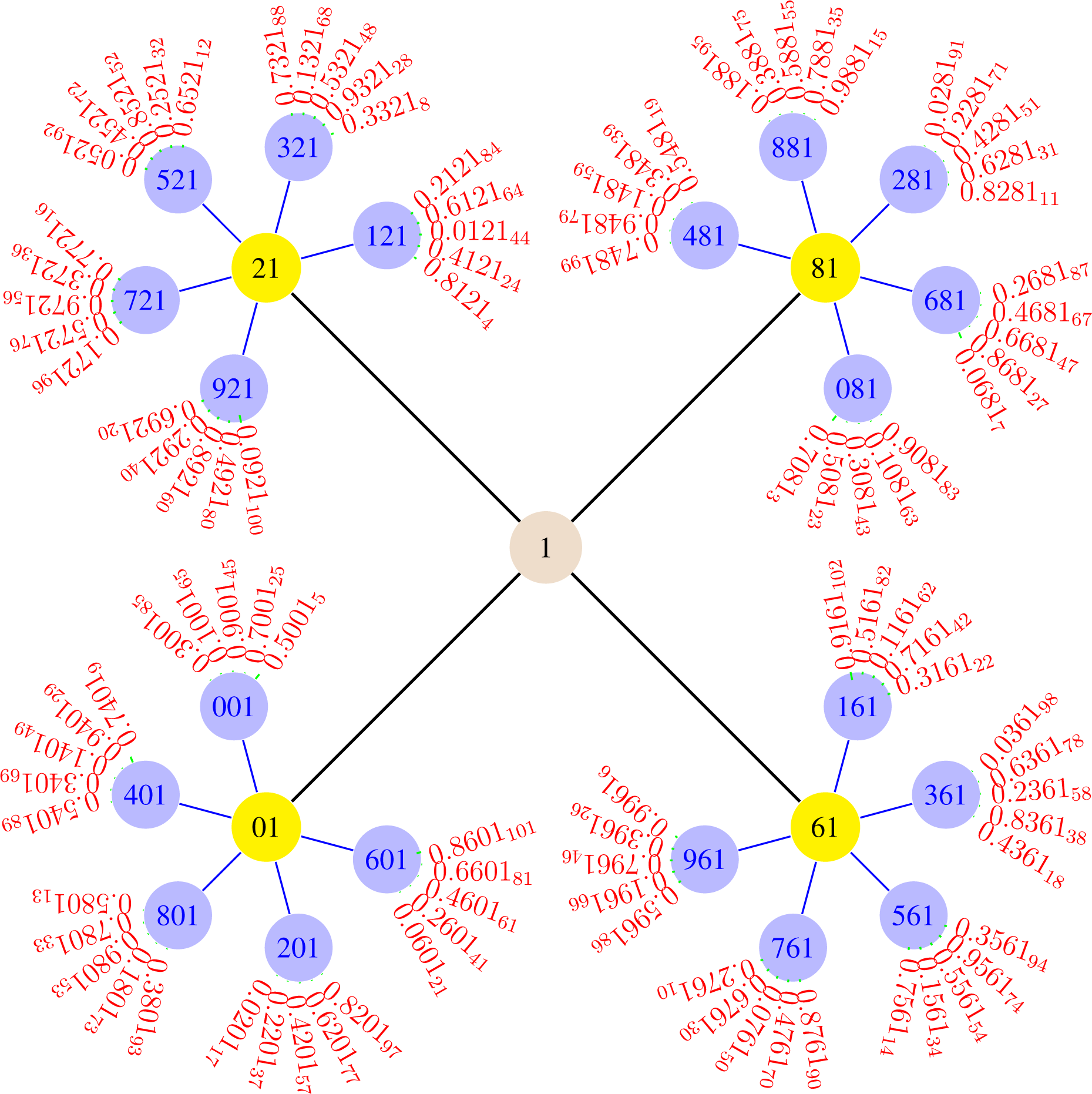
Figure 1 shows the structure of the lower four positions of TNSs for
x0 = 0.1 and
a = 3.9.
The position located in the last positions of TNSs is called the root gene position, when the value of the root gene positions in the cycle part is invariable. For example, when
x0 = 0.1,
a = 3.9 and
pn = 4, the root gene position is the last position of TNSs. In
Figure 1, the root gene position is located in the center. Its value is equal to one.
When the period of the lower positions is equal to four, the positions are called the common gene position (CGP). For example, in
Figure 1, the last two positions are the common gene positions,
i.e., “21”, “81”, “01” and “61”. Others are called the individual gene position (IGP).
In
Figure 1, every individual gene position varies in the set
Zodd = {1, 3, 5, 7, 9} and the set
Zeven = {0, 2, 4, 6, 8}. For example, the individual gene position with the common gene positions “81” is “081”, “681”, “281”, “881” and “481”, which belong in the set
Zeven. The individual gene position with the common gene positions “21” is “121”, “321”, “521”, “721” and “921”, which belong in the set
Zodd.
Note that every iteration with the individual gene position moves from one common gene position to another. For example, for
x0 = 0.1,
a = 3.9 and
pn = 3,
x17 = 0.201 with the individual gene position “2” and the common gene positions “01” moves to
x18 = 0.361 with the common gene positions “61”. In
Figure 1, x9 = 0.7401 with the individual gene positions “74” and the common gene positions “01” moves to
x10 = 0.2761 with the common gene positions “61”.
We take another example to investigate the property of lower positions. Assume that x0 = 0.3 and a = 3.4; the true numerical solutions are listed as follows.
x1 = 0.714.
x2 = 0.6942936.
x3 = 0.721649989796736.
x4 = 0 682⋯5727374336.
x5 = 0.736⋯1171009536.
x6 = 0.660⋯4300199936.
x7 = 0.762⋯4470260736.
We provide the upper three positions and the lower ten positions of the true numerical solutions from x4 to x7. Some middle positions are omitted, because the situation has no effect on observing lower positions of the true numerical solutions. As seen above, the lower three positions of TNSs are listed as follows.
Note that the regularity occurs in the lower three positions. The length of period is equal to four. For x0 = 0.3 and a = 3.4, the root gene positions are the last two positions, i.e., “36”. The common gene positions are “936”, “736”, “336” and “536”.
We increase the value of lower pn positions. Assume that x0 = 0.3, a = 3.4 and pn = 4. The lower four positions of TNSs are listed as follows.
As seen above, the individual gene position with the common gene positions “736” is “6736”, “0736”, “4736”, “8736” and “2736”, which belong in the set Zeven. The individual gene position with the common gene positions “936” is “1936”, “3936”, “5936”, “7936” and “9936”, which belong in the set Zodd.
Assume that
cpn=η is the length of the period with the lower
pn positions, where
pn is equal to
η. From
Table 1, we can see that when the length of the period is greater than four and the individual gene position increases by one digit position, the new length of period will be five-times as long as the original length of period.
In order to further verify the regularity, we take values of the control parameter of a ∈ {3.1, 3.2, 3.3, 3.4, 3.6, 3.7, 3.8, 3.9}, and initial values of x0 ∈ {0.1, 0.2, 0.3, 0.4, 0.6, 0.7, 0.8, 0.9}.
When a is specified, the value of x1 is the same for the initial values of x0 = 0.1 and x0 = 0.9, x0 = 0.2 and x0 = 0.8, x0 = 0.3 and x0 = 0.7, x0 = 0.4 and x0 = 0.6, respectively. Therefore, we give, for example, (x0 = 0.1, a) and omit (x0 = 0.9, a).
The length of the period is summarized in
Table 2. Experimental results by the initial conditions are divided into three groups in the form of (
x0,
a):
Group 1 = {(0.1, 3.1), (0.4, 3.2), (0.1, 3.3), (0.2, 3.3), (0.3, 3.4), (0.3, 3.8)};
Group 2 = {(0.2, 3.1), (0.3, 3.7)};
Group 3 = {(0.1, 3.2), (0.1, 3.4), (0.1, 3.6), (0.1, 3.7), (0.1, 3.8), (0.2, 3.2), (0.2, 3.4), (0.2, 3.6), (0.2, 3.7), (0.2, 3.8), (0.2, 3.9), (0.3, 3.1), (0.3, 3.2), (0.3, 3.3), (0.3, 3.6), (0.3, 3.9), (0.4, 3.1), (0.4, 3.3), (0.4, 3.4), (0.4, 3.6), (0.4, 3.7), (0.4, 3.8), (0.4, 3.9)}.
For x0 = 0.2 and a = 3.1 in Group 2, the lower four positions of TNSs are listed as follows.
For x0 = 0.2, a = 3.1 and pn = 4, the root gene positions are the last three positions, i.e., “504”. When the length of the period is equal to four, it is called the critical point of the period.
From
Table 2, the situation is similar in that the new length of the period is five-times as long as the original length of the period when the individual gene position increases by one digit position. This implies that the length of the period will enlarge for the same initial conditions and control parameter when the individual gene positions increase.
When lower pn positions are specified, the less the number of the root gene position is, the larger the length of period will be. For example, assume that the lower positions are set to four. For x0 = 0.2, a = 3.1 and pn = 4 in Group 2, the length of the period is equal to four. The root gene position occupies three digital positions, i.e., “504”. For x0 = 0.3, a = 3.4 and pn = 4 in Group 1, the length of the period is equal to 20. The root gene position occupies two digital positions, i.e., “36”. For x0 = 0.1, a = 3.9 and pn = 4, the length of the period is equal to 100. The root gene position occupies a digital position, i.e., “1”.
For
a = 3.9,
x0 = 0.2 and
pn = 4, the lower four positions of the true numerical solutions in the real orbit become the period starting from
x2 to
x102. The length of period is equal to 100. The individual gene positions with the common gene positions are shown in
Table 3.
The numerical solution represents 0.r1r2r3r4 for a = 3.9, x0 = 0.2 and pn = 4. The root gene position is the digit position r4, which is equal to six. The combined digit positions of r3 and r4 are the common gene positions, which are equal to “36”, “56”, “96” and “76”. The digit positions r1 and r2 stand for the first position and the second position of the individual gene positions.
The randomness of IGPs of the true numerical solutions in the real orbit is shown in
Table 4. The permutation and combination values of
r1 and
r2 range from 00 to 99. It is obvious that the combined individual gene positions of
r1 and
r2 are different from each other and impinge on all points in the given space. In fact, the property of the logistic map derives from the individual gene positions. In other words, the individual gene positions exhibit the ergodicity and randomness of the logistic map.
Table 5 shows the property of the half-life of the logistic map. For example, the first column of
Table 4 shows the length of the period with the common gene position “36” equal to 25. The same situation happens in the second, third and fourth columns of
Table 4. From
Table 5, we can see that when the individual gene positions increase, the length of the period with the same common gene positions has the property of the half-life. The reason is that each digital position of the individual gene positions varies in the sets
Zodd and
Zeven.
The property of the half-life is the nature of the logistic map, which is independent of computational errors in computers. Therefore, the numerical solutions with computational errors could interfere with the nature of nonlinear dynamics.


