Application of Entropy and Fractal Dimension Analyses to the Pattern Recognition of Contaminated Fish Responses in Aquaculture

Abstract

The objective of the work was to develop a non-invasive methodology for image acquisition, processing and nonlinear trajectory analysis of the collective fish response to a stochastic event. Object detection and motion estimation were performed by an optical flow algorithm in order to detect moving fish and simultaneously eliminate background, noise and artifacts. The Entropy and the Fractal Dimension (FD) of the trajectory followed by the centroids of the groups of fish were calculated using Shannon and permutation Entropy and the Katz, Higuchi and Katz-Castiglioni’s FD algorithms respectively. The methodology was tested on three case groups of European sea bass (Dicentrarchus labrax), two of which were similar (C1 control and C2 tagged fish) and very different from the third (C3, tagged fish submerged in methylmercury contaminated water). The results indicate that Shannon entropy and Katz-Castiglioni were the most sensitive algorithms and proved to be promising tools for the non-invasive identification and quantification of differences in fish responses. In conclusion, we believe that this methodology has the potential to be embedded in online/real time architecture for contaminant monitoring programs in the aquaculture industry.

1. Introduction

Biological systems, such as a group of animals, are regulated by interacting mechanisms that operate across multiple spatial and temporal scales. When studying such a biological system, we are interested, as defined by Kitano [1], in how the large numbers of functionally diverse and multifunctional set of elements (i.e., the individual animals in our case) interact selectively and nonlinearly to produce coherent rather than complex behaviours.

The output variables from biological systems usually have complex fluctuations, which contain valuable information about their intrinsic dynamics. Signals and noise are the basic components of signal and data analysis, but most of the time series generated by biological systems contain both deterministic and stochastic components [2]. Classical approaches are not able to quantify the complexity of these systems, this is why real world applications and noisy environments often require alternative techniques leading to improved systems. Thus, the combination of nonlinear and linear modelling and/or features has led to higher and more robust performance, something particularly promising for solving complex tasks in real environments [3].

One of the main goals of applied mathematics and computing in modern biology is to capture all the richness of complex biological systems into theoretical models [1,4]. Fractal analysis has found a wide area of applications in a variety of scientific fields from medicine [5–7] to speech recognition [8], walking pattern recognition [9], stress indicators in goats [10] and in fish motion studies [11–13]. The Fractal Dimension (FD) of a system is one of the most significant features to describe its complexity. Fractal systems have a characteristic called self-similarity, i.e., a close-up examination of the system reveals that it is composed of smaller versions of itself. Self-similarity can be quantified as a relative measure of the number of basic building blocks that form a pattern, and this measure is defined as the FD, which is rarely an integer number. Usually, the more complex the signal, the higher its FD value [14]. FD analysis has been successfully applied by López-de-Ipiña [15] to speech analysis and by Nimkerdphol and Nakagawa [16] to show quantitative differences in the swimming behaviour of zebrafish provoked by the presence of hypochlorite in the water.

The Entropy of a system is also a nonlinear measurement that has found application in complex biological systems and has occasionally been decisive to understand the nonlinear nature of a problem. For instance, Kulish et al. [17] analyzed brain activity using the spectra of the FD based on the Renyi entropy: combined with a visualization tool, these authors showed an intrinsic asymmetry of the brain activity. Permutation entropy has been used in a wide range of applications where measurement of complex time series where needed. As an example Li [18] measured the effects of sevofluore on the the complexity in electroencephalographic series, Liu et al. [19] analysed the movement of the fruit fly and Bandt and Pompe [20] studied the complexity of chaotic time series.

Non-invasive pattern analysis of the responses of animals to unexpected events may have application in several fields, including monitoring of animal welfare and detection of contaminants, air pollutants or oxygen availability in closed environments. In contrast to analyzing the behavior, which is a very complex and species-specific attribute, the immediate response to a stochastic event is simpler, requires less computational power and once a suitable methodology is developed we believe that it will require less modifications in order to be applicable to other species and settings.

The animal case selected for this work was fish due to the worldwide spectacular increase in aquaculture production. This increase has created a need to non-invasively monitor and control relevant variables during the production, in particular those relating to seafood safety and to the welfare and health of the fish. Some studies have been conducted to build up machine-based systems for fish disease diagnosis. In those studies the main challenge is to develop the knowledge database, a task which is time and resource consuming and focuses mainly on water quality [21] and/or on nutritional problems, parasites, viruses, bacteria and fungal agent diseases [22]. Other studies aim at developing early warning systems [23], including the use of sms alert procedures [24]. The main challenge for these fish-health oriented studies is the development of the decision component rather than the warning systems itself.

In addition, suboptimal environmental conditions, such as hypoxia, feeding regime [25], high fish density [26,27], the presence contaminants in the water including human drugs [28] and hypochlorite, and the water’s pH [16] have been shown to alter fish behaviour. This opens the possibility of using fish behaviour itself as a biomarker for environmental monitoring and in aquaculture settings. Fish behaviour is very complex [29] and the response to a stochastic event may be considered one aspect of it. Following Kitano’s idea [1], we were interested in studying the coherent response of the group rather than the individual response of each fish, which in addition to requiring much more computational effort it may be impractical in real-life settings where there may be several thousand individuals in the same area or cage.

The objective of the present work was to develop a methodology for image acquisition, processing and nonlinear trajectory analysis of the collective fish response to a stochastic event. The acquisition of the information of the movement of the fish can be achieved by images, typically video recording [30–32] and/or by echo-sounds [25]. The information thus obtained may then be processed by different nonlinear algorithms as indicated above. Video recording was chosen for its simplicity and FD and Entropy for their proven suitability to identify nonlinear features.

2. Materials and Methods

2.1. Experimental Cases

Three experimental cases were used to test the methodology: C1 and C2, consisting of 81 fish each and differing only in that C2 fish were tagged with Visual Implant Elastomer by Northwest Marine Technology [33] and C3 with 41 fish that had been treated for 9 days with 4 μg methylmercury/L. During all the experimental period the fish were subject to a 12h /12h dark/light photoperiod and they were fed once a day INICIO Plus feed from BioMar (56% crude protein, 18% crude fat). The fish were placed in tanks (100 cm × 100 cm × 90 cm) filled up to 80.5 cm of height with 810 L of aerated seawater under direct light (2 × 58 W and 5200 lumen) avoiding shadows as much as possible. To record the fish response one camera was placed in each tank positioned exactly in the same place.

The experimental procedure was approved by The Ethical Committee for Animal Welfare No. CEBA/285/2013MG. The fish were European sea bass (Dicentrarchus labrax, 4 ± 2 g, 8 ± 1 cm) generously provided by Grupo Tinamenor (Cantabria, Spain).

2.2. Image Acquisition and Pre-Processing

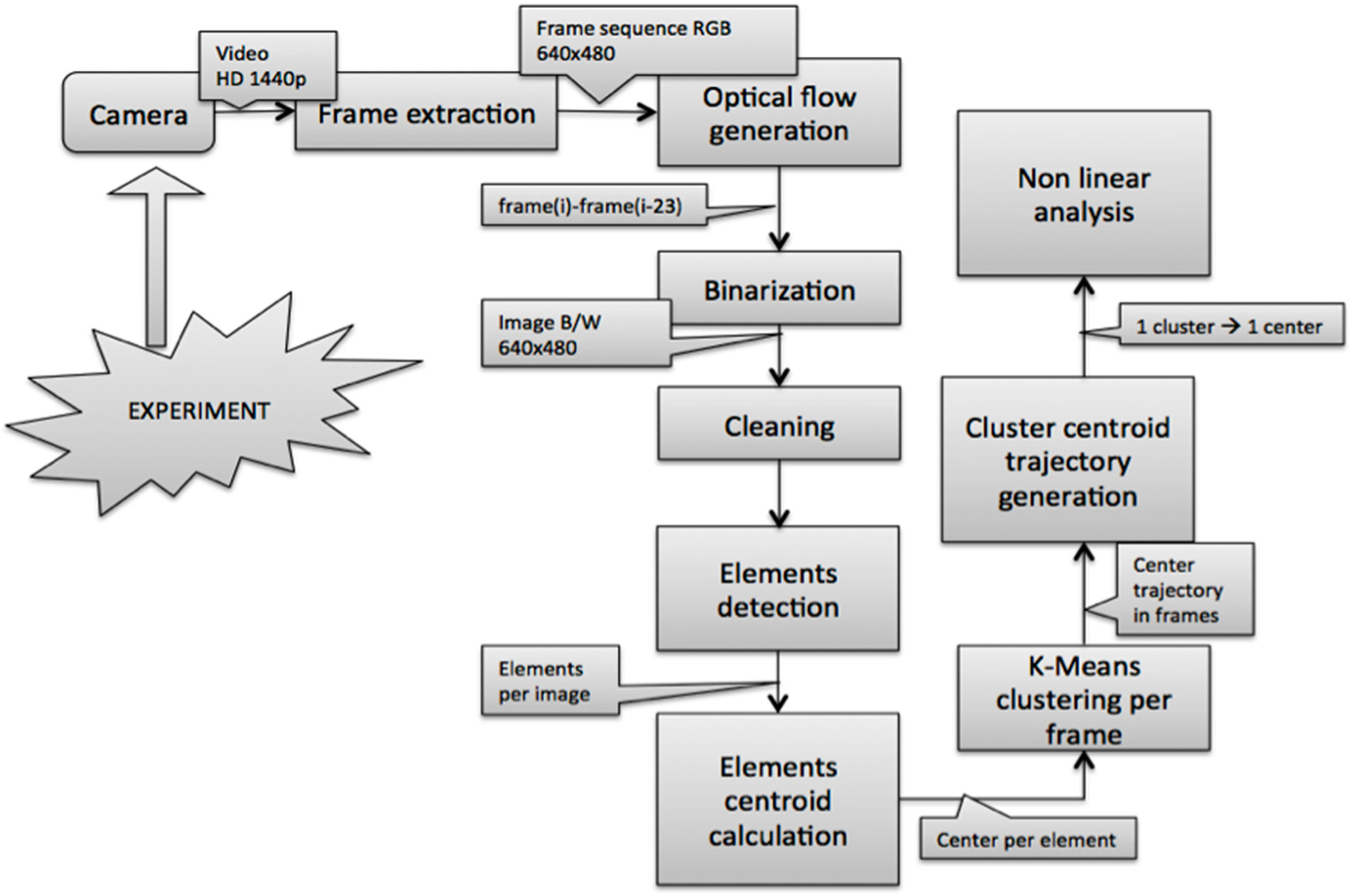
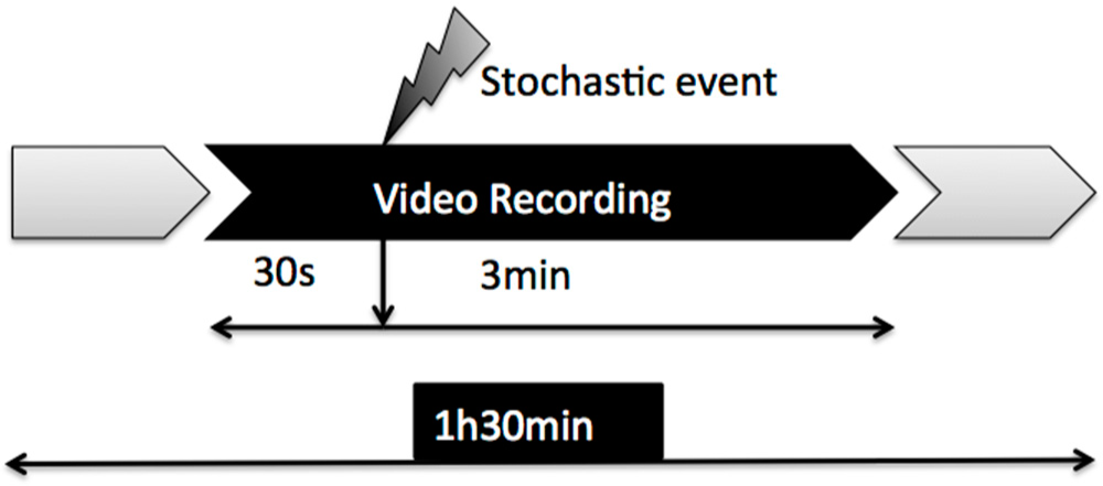
The schematic diagram of the working procedure is described in Figure 1. The video sequences and images were acquired using a GoPro Hero3 high definition camera in its GoPro Underwater housing attached to the tank by GoPro Side and Flat mounts placed in the top right corner of the tank just 3.8 cm from the right wall, 15 cm from the top of the tank and 5.5 cm below water level. This camera was used for convenience: its size is small, thus minimizing the effect of introducing foreign objects in the tank, and it has a water-proof protective case very convenient because it has to be submerged in contaminated water, so that at the end of the experiment the camera can be reused while the case is discarded as contaminated material. The recordings were made in high definition RGB scheme at 1440p, 24 frames per second (fps) and in 16:9 picture size. For the recording a SanDisk 32 Gb Ultra microSDHC™ (Class 10) secure card was used and for post-storing a 2 Tb Hard Disk. In order to minimize stressing factors, continuous recordings were done until the batteries of the cameras run out, which was about 1 h and 30 min. Within this period, a stochastic event consisting of a sudden hit in the tank was introduced and the 30 s pre- and 3 min post-event were processed (Figure 2).

The 3 min 30 s of interest were located using the sound clip of each video analyzed with Audacy free software to determine exactly where the event happened. The 3 min 30 s clip was cut from the main video and converted into a sequence of images. Since the video was recorded at 24 fps it was converted also to 24 fps. The images were compressed from the 1440p HD format to the more convenient 640 pixel × 480 pixel format. Frame extraction and format conversion were made with the commercial iMovie software. After the video was converted into a color image sequence, the background and noises were eliminated and it was then converted to black and white.

2.3. Detection of Objects and Motion Estimation

From the point of view of image segmentation and object detection, and due to the nature of the set up, (a biological experiment in a real, small-scale industrial environment) there were three main problems: noise, artefacts and occlusions.

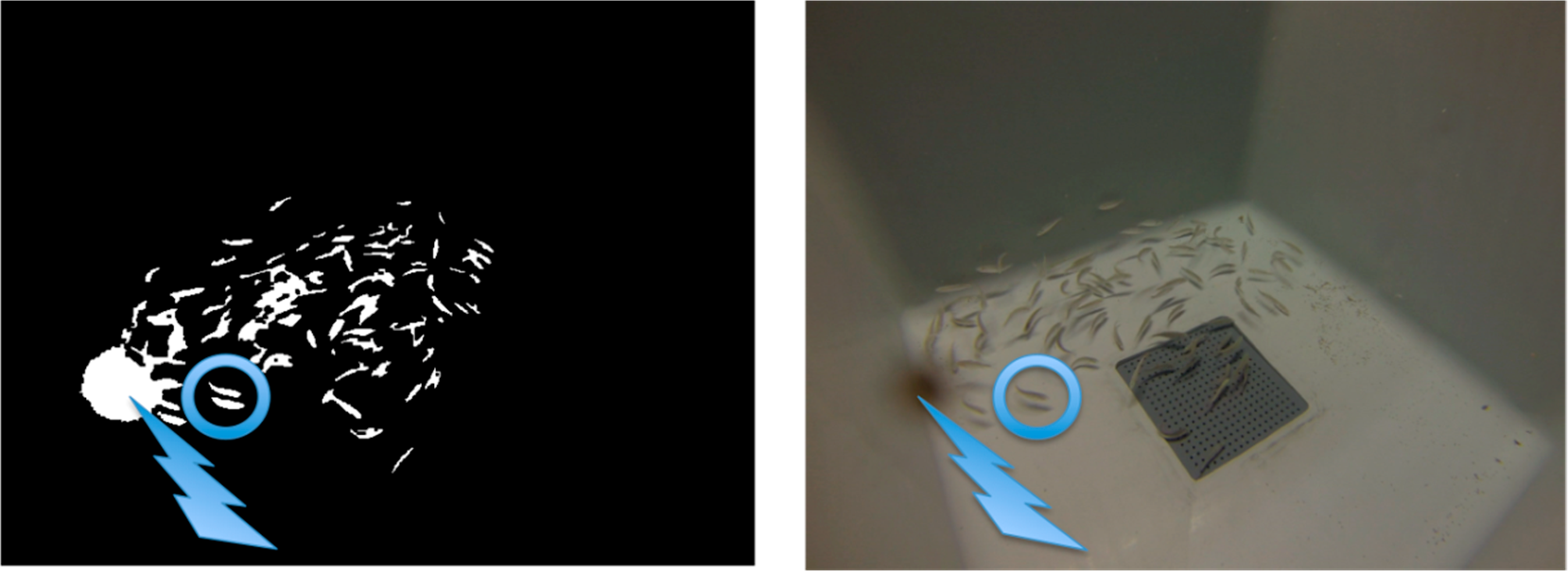
Two main sources of noise were identified: air bubbles and shadows. The main noise was generated by the air bubbles moving towards the surface. This creates a little wave system on the water surface, which makes the light penetrate the water in a nonlinear manner. The second noise source was the shadows of the fish on the bottom and the tank’s walls. Although the lighting was placed on the ceiling above the tank to avoid this issue, the generation of some shadows was unavoidable (see Figure 3).

There were three main types of artefacts (anomalies introduced in the signal or in the data by the equipment or the technique): the first was caused by the pellets used for feeding the fish. Some food pellets were suspended in the water and when fish swam around them, they spread off forming black holes in the images (see Figure 3). The second (very similar to the first but smaller in size) was caused by the faeces of the fish, and the third by the light’s reflections on the skin of the fish.

Occlusions are a well-known issue in tracking that occur when two or more tracked target images become one during a time period in the sequence. Occlusions are more frequent when target objects are similar to each other, as it happens in animal groups and fish [34]. Occlusions in fish tracking may lead to two types of misidentification: loss of fish identity and swapping identity between individuals [31]. Tracking problems take place both while the occlusion occurs and when the occlusion ends and the fish appear separately in the image. To solve this problem different solutions have been developed such as the use of 3D information [35,36], using the animals’ characteristics, such as its shape [37–39] or analyzing the special topology of the shape [40–43]. Automatic scene calibrating systems are also very helpful tools and many approaches have been made in this field, for example an automatic calibrating camera system for tracking people [44].

Given that the robustness of the system depends on how the motion detection takes place and all the problems listed above severely limit the election of the motion estimation algorithm, we decided to use an algorithm based on optical flow in order to eliminate noise, artefacts and occlusions in one step. This conventional approach is based on the calculation of the local relative motion [45] which is also used for space segmentation [46], and it has the additional advantage that it can work with a moving camera and/or with moving backgrounds. We applied this method to detect objects and estimate their motion by a simple process which consisted in identifying the differences between one of the images and the image obtained in the previous second, i.e., resting each frame from its 24th predecessor (since we work at 24 fps). This made it possible to delete background, noise and artifacts common to all images, including objects that had not changed position in the previous second while keeping those objects whose position changes in 1 second intervals, i.e., the moving fish. Methods based on optical flow provide very valuable information but they are computationally intense and sometimes require specific hardware.

After the optical flow, or motion, was calculated, the images were binarized using standard morphologic operations in order to be able to detect the elements in the image and their centers in each frame.

2.4. Clustering and Trajectory Generation

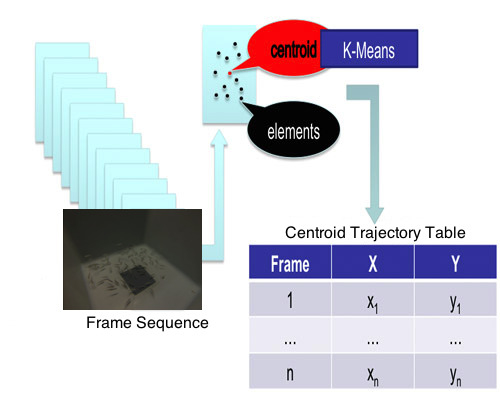
In order to work in the most reliable way possible, knowing that our system, experiment and conditions have limitations and being particularly concerned about a potential loss of information due to the image segmentation and processing methods, we decided to use a clustering method to identify the fish group and calculate the group’s centroid.

The centroids’ positions were estimated by k-means because this algorithm is robust, with a good relationship between speed and stability and it works well with large amounts of data. Thus, once the centers of the objects were calculated, and knowing their coordinates in the two axes within each frame, k-means was applied to find the center of the entire group. In our particular case, the dataset were the objects’ centers in each frame, from the first frame to the last one. K-means clustering operates on actual observations (rather than on a larger set of dissimilarity measures), and creates a single level of clusters. K-means then treats each observation in the data set as an object having a location in space. It finds a partition in which objects within each cluster are as close to each other, and as far from objects in other clusters, as possible. Depending on the kind of data to cluster, it is possible to use up to five different methods to calculate the distances. The best results for the current problem were obtained using the Euclidean distance [47,48].

Each cluster in the partition was defined by its member objects and by its centroid, or center: the point where the sum of distances from all objects in the cluster is minimized. K-means computes the cluster’s centroids differently for each distance measured in order to minimize the sum with respect to the distance specified. This is done using an iterative algorithm that minimizes the sum of the distances from each object to its cluster’s centroid, over all clusters. The algorithm moves objects between clusters until the sum cannot be decreased further. The result is a set of clusters that are as compact and separated as possible. It is possible to control the details of the minimization using several optional input parameters to k-means, including the initial values of the cluster centroids, and the maximum number of iterations. This algorithm, often applied for image segmentation, has successfully been used to detect animals [48]. The centers of the clusters are calculated in a two space dimension (2D), using both coordinates (X and Y) and the frame number, which goes from 1 to n in the image sequence, and then a trajectory table is built (

Table 1. The cluster’s centroid coordinates are calculated for each frame and from them the trajectory of the cluster is calculated.

Frame Number	X Coordinate	Y Coordinate	Centroid’s Coordinates
1	x1	x	x1,y1
2	x2	y2	x2,y2
…	…	…	…
n	xn	yn	xn,yn

).

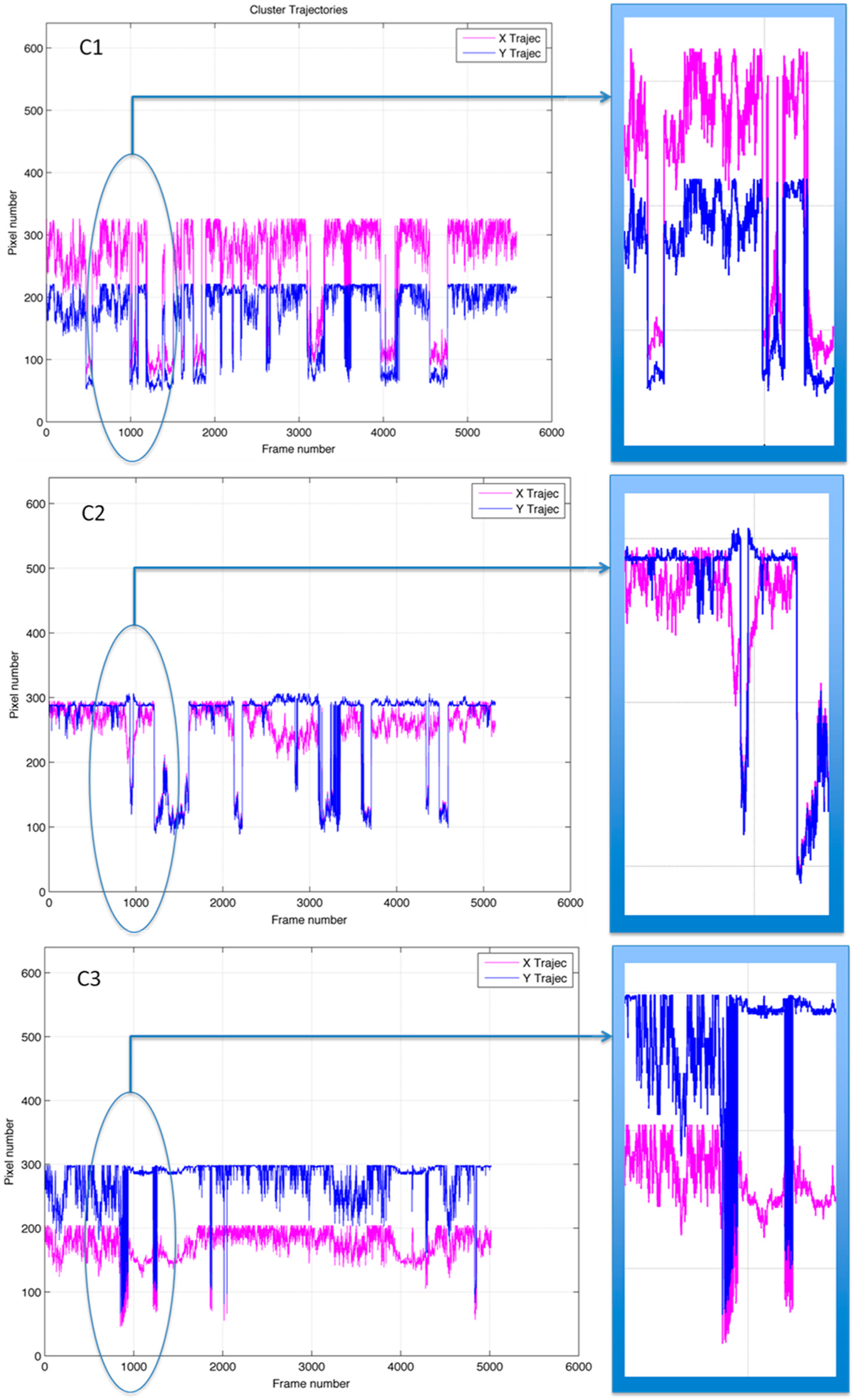
A new figure (Figure 4) was then created by plotting the values obtained from Table 1: in the vertical axes the values corresponding to the pixel number of the x-coordinate of the centroid (in red) and to the pixel number of the y-coordinate of the centroid (in blue) and in the horizontal axis the frame number to which each x and y values correspond. Since the images have a 640 pixel × 480 pixel format, the scale of the vertical axis in Figure 4 goes from 0 to 640 pixel number (the lowest and highest theoretical possible value for the x-pixel number in Table 1, when the centroid is placed either in the border right or border left of the frame). The lowest and highest theoretical possible value for the y-pixel number in Table are 0 and 480 respectively. The horizontal axis, representing the frame number varies in the three cases due to the processing of the video sequences. In all three cases there was a sharp change in the trajectory of the centroid in response to the stochastic event, which occurs around frame number 720. The panels to the right in Figure 4 show a magnification of the region of the plot corresponding to the response to the event.

2.5. Fractal Dimension (FD)

Among the various algorithms available to measure the FD, we selected those specially suited to time series analyses that don’t need previous modelling of the system. Two of those algorithms are Higuchi [49] and Katz [50] named after their authors. We used the former as the main reference, and a modification proposed by Castiglioni [51] on the original version developed by Katz [50]. Higuchi was our first choice because it has been reported to be more accurate [52] but in most of these studies, the algorithm compared to was the original one developed by Katz himself. Castiglioni’s improvement is theoretically sound and has not been tested in many experiments, so we considered interesting to test as an alternative.

The algorithm proposed by Higuchi [49] measures the FD of discrete time sequences directly from the time series {x₁,x₂,…,x_n}. The algorithm calculates the length L_m(k) for each value of m and k, where m is initial time {m = 1,2,…,k} and k is time interval {m = 1,2,…,k_max}. N is the lenght of the sampled signal.

$${\mathrm{L}}_{\mathrm{m}}(\mathrm{k})=\frac{{{\displaystyle \sum }}_{\mathrm{i}=1}^{\frac{\mathrm{N}-\mathrm{m}}{\mathrm{k}}}|\mathrm{x}(\mathrm{m}+{\mathrm{i}}_{\mathrm{k}})-\mathrm{x}(\mathrm{m}+(\mathrm{i}-1)\mathrm{k})|(\mathrm{N}-1)}{\lfloor \frac{\mathrm{N}-\mathrm{m}}{\mathrm{k}}\rfloor \mathrm{k}}$$

(1)

After that, a sum of all the lengths L_m(k) for each k is determined by:

$$\mathrm{L}\left(\mathrm{k}\right)={\displaystyle \sum }_{\mathrm{m}=1}^{\mathrm{k}}{\mathrm{L}}_{\mathrm{m}}\left(\mathrm{k}\right)$$

(2)

And finally, the slope of the curve ln(L(k)) ⁄ln(1⁄k) is estimated using the best fit by linear least squares. The result is the Higuchi FD.

On the other hand, Katz [50] proposed a normalized formula of the FD:

$$\mathrm{FD}=\frac{\log (\mathrm{n})}{\log (\mathrm{n})+\log (\mathrm{d}/\mathrm{L})}$$

(3)

where the length L and the extension d of the curve are normalized using the average step a = L/n using (4) and (5).

$$\mathrm{L}={\displaystyle \sum }_{\mathrm{i}=1}^{\mathrm{n}}{\mathrm{l}}_{\mathrm{i},\mathrm{i}+1}$$

(4)

$$\mathrm{d}=\max \left\{{\mathrm{l}}_{\mathrm{i},\mathrm{j}}\right\}$$

(5)

Nevertheless, given that the input signal is a mono-dimensional waveform, the length and the extension can be rewritten using Mandelbrot’s approach [53]. A simple and efficient way to do this is directing these two magnitudes in their own dimension as it was done by Castiglioni [51]. One by one, the extension on the Y axis is the range of y_k as seen in:

$$\mathrm{d}=\max \left\{{\mathrm{y}}_{\mathrm{k}}\right\}-\min \left\{{\mathrm{y}}_{\mathrm{k}}\right\}$$

(6)

and the length L is the sum of all the increments in modulus as in:

$$\mathrm{L}={\displaystyle \sum }_{\mathrm{k}=1}^{\mathrm{n}}\left|{\mathrm{y}}_{\mathrm{k}+1}-{\mathrm{y}}_{\mathrm{k}}\right|$$

(7)

This latter calculation is what is called the Castiglioni’s variation of Katz’s algorithm [51].

Once the FD algorithms were selected, it was extremely important to choose the window size to be used for the calculations. The fractal window goes through the signal, i.e., the object to analyze. This sliding window has a fixed size during each analyzing period. In order to calculate the FD’s features of the signal there are no restrictions other than the total waveform length to the window size to be used. Each signal was analyzed using three fixed, but configurable, window lengths: 320 points, 640 points and 1280 points. The third window size of 1280 points was tested because previous studies that take into account the window size of similar dimension estimations [52,54] suggest that a bigger window could be useful in some cases. Since the FD is a tool intended to capture the dynamics of the system, with a short window the estimation would be very local and adapting fast to the changes in the waveform. When the window is longer, some details will be lost but the FD anticipates better the characteristics of the signal [8].

Each of the three experimental cases, C1, C2 and C3, were treated by Higuch, Katz, and the Castiglioni’s variation of Katz’s algorithm using window lengths of 320, 640 and 1280 points.

2.6. Shannon Entropy

Entropy is the measure of disorder in physical systems. The entropy H(X) of a single discrete random variable X is a measure of its average uncertainty. Shannon entropy [55] is calculated by the equation:

$$\mathrm{H}(\mathrm{X})=-{\displaystyle \sum }_{{\mathrm{x}}_{\mathrm{i}}\mathrm{\in \Theta }}\mathrm{p}({\mathrm{x}}_{\mathrm{i}})\log \mathrm{p}({\mathrm{x}}_{\mathrm{i}})=-\mathrm{E}[\log \mathrm{p}({\mathrm{x}}_{\mathrm{i}})]$$

(8)

where X represents a random variable with a set of values Θ and probability mass function p(x_i) = P_r {X = x_i}, x_i ϵ Θ, and E represents the expectation operator. Note that p logp = 0 if p = 0.

For a time series representing the output of a stochastic process, that is, an indexed sequence of n random variables, {Xi} = {X₁,…, X_n}, with a set of values θ₁,…,θ_n, respectively, and Xiϵθ_i, the joint entropy is defined by:

$${\mathrm{H}}_{\mathrm{n}}=\mathrm{H}\left({\mathrm{X}}_1,\dots ,\mathrm{Xn}\right)=-{\displaystyle \sum }_{{\mathrm{x}}_{\mathrm{i}}\mathrm{\in \theta }}\dots {\displaystyle \sum }_{{\mathrm{x}}_{\mathrm{n}}{\mathrm{\in \theta }}_{\mathrm{n}}}\mathrm{p}\left({\mathrm{x}}_1,\dots ,{\mathrm{x}}_{\mathrm{n}}\right)\log \mathrm{p}\left({\mathrm{x}}_1,\dots ,{\mathrm{x}}_{\mathrm{n}}\right)$$

(9)

where p(x₁,…x_n)=P{X₁=x₁,…,X_n=x_n} is the joint probability for the n variables X₁,…,X_n.

By applying the chain rule to Equation (9), the joint entropy can be written as a summation of conditional entropies, each of which is a non-negative quantity:

$${\mathrm{H}}_{\mathrm{n}}={\displaystyle \sum }_{\mathrm{i}=1}^{\mathrm{n}}\mathrm{H}\left({\mathrm{X}}_{\mathrm{i}}|{\mathrm{X}}_{\mathrm{i}-1},\dots ,{\mathrm{X}}_1\right)$$

(10)

Therefore, it concludes that the joint entropy is an increasing function of n. The rate at which the joint entropy grows with n, i.e., the entropy rate h, is defined as:

$$\mathrm{h}=\underset{\mathrm{n}\to \infty }{\lim }\frac{{\mathrm{H}}_{\mathrm{n}}}{\mathrm{n}}$$

(11)

For stationary ergodic processes, the evaluation of the rate of entropy has proved to be a very useful parameter [56–61]. The Shannon entropy was calculated from the same trajectory signals of the clusters’ centroid for both axis, X and Y, which had been used to estimate the FD shown in Figure 4.

2.7. Permutation Entropy

As Shannon entropy, permutation entropy quantifies the disorder of a system. It has shown a good ability to measure complexity for large time series and basically this method converts a time series into an ordinal patterns series where the order of relations between the present and a fixed number of equidistant past values at a given time are described [19,62].

Following this idea, Bandt and Pompe [20] proposed a permutation entropy method based on the Shannon entropy measurement with the purpose of visualizing and quantifying changes in the time series. The permutation entropy is calculated for a given time series{x₁,x₂,…,x_n} as a function of the scale factor s. In order to be able to compute the permutation of a new time vector X_j, S_t = [X_t, X_t+1,…,X_t+m−1] is generated with the embedding dimension m and then arranged in an increasing order: $\left[X_{t+j_1-1}\le X_{t+j_2-1}\le \dots \le X_{t+j_n-1}\right]$. Given m different values, there will be m! possible patterns π, also known as permutations. If f (π) denotes its frequency in the time series, its relative frequency is p(π) = f(π)/(L/s−m+1). The permutation entropy is then defined as:

$$PE=-{\displaystyle \sum }_{i=1}^{m!}p({\pi }_i)\ln p({\pi }_i)$$

(12)

Summarising, permutation entropy refers to the local order structure of the time series, which can give a quantitative measure of complexity for dynamical time series. This calculation depends on the selection of the m parameter, which is strictly related with the length N of the analysed signal. For example Bandt and Pompe [20] suggested the use of m = 3,…,7 following always this rule:

$$m!<N$$

(13)

If m is too small (smaller than 3) the algorithm will work wrongly because it will only have few distinct states for recording. When using long signals, a large value of m is preferable but it would require a larger computational time.

In our particular case and due to the computational cost derived from analysing signals composed from 5000 samples, the m parameter was fixed at a value of m = 4.

3. Results and Discussion

The non-invasive tool we wished to develop targeted the responses of the fish groups rather than that of individual fish both to reduce the computational effort and because the response of the group may be considered the result of integrating all the responses each individual fish, which may be influenced by the physiological status of the individual, its size, status in the school’s hierarchy and other factors that are usually unknown in monitoring purposes. Also, the response to a stochastic event was measured instead of other behavioural aspects (swimming pattern, daily activity, feeding, aggressiveness, etc.) because it permits to restrict the computational analysis in time to the duration of the response (three minutes was sufficient in our case, rather than observing the animals for longer periods of time where more variables may play a role) and to reproduce the event at will in other settings for comparison purposes. Longer periods of time were also analyzed but the discriminative power of the analyses did not improve (results not shown).

Of the three cases examined, we expected C1 and C2 to behave similarly to each other and to be clearly different from C3 due to the methylmercury contamination in C3. The neurotoxic agent methylmercury was selected because of its increasing relevance as an environmentally ubiquitous pollutant that accumulates and biomagnifies in the trophic chain [63]. Although differences in fish stocking density between C1 and C2 (81 fish) vs C3 (41 fish) might have had an effect on the responses to the event, most probably they did not [26,27].

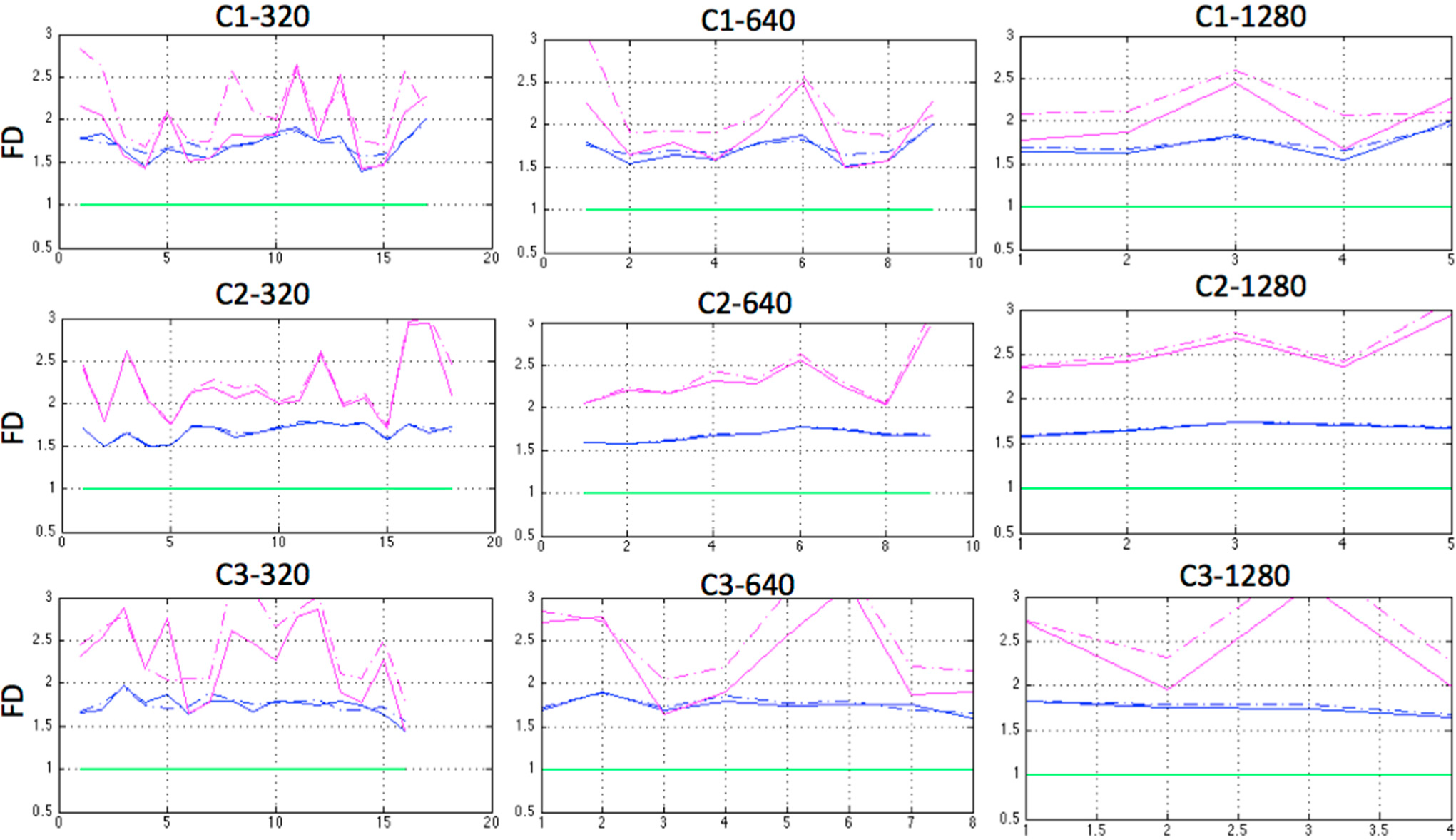
Two of the three FD algorithms used, Higuchi and Katz’s variation proposed by Castiglioni were able to differentiate C1, C2 and particularly C3, for the three sampling window lengths in both coordinates of the clusters’ centers, X and Y in a 2D analysis, as shown in Figure 5. Since there was a correlation between the X and Y coordinates, the rest of the calculations were performed on only one of them, the X values. The almost constant and close to 1 value of the FD obtained by using the Katz algorithm is in agreement with the results of Raghavendra [64] and confirms Castiglioni’s note [51].

Indeed the modification proposed by Castiglioni was more sensitive to detect differences between the three cases than Higuchi, suggesting that for our particular application, it may be the most suitable algorithm.

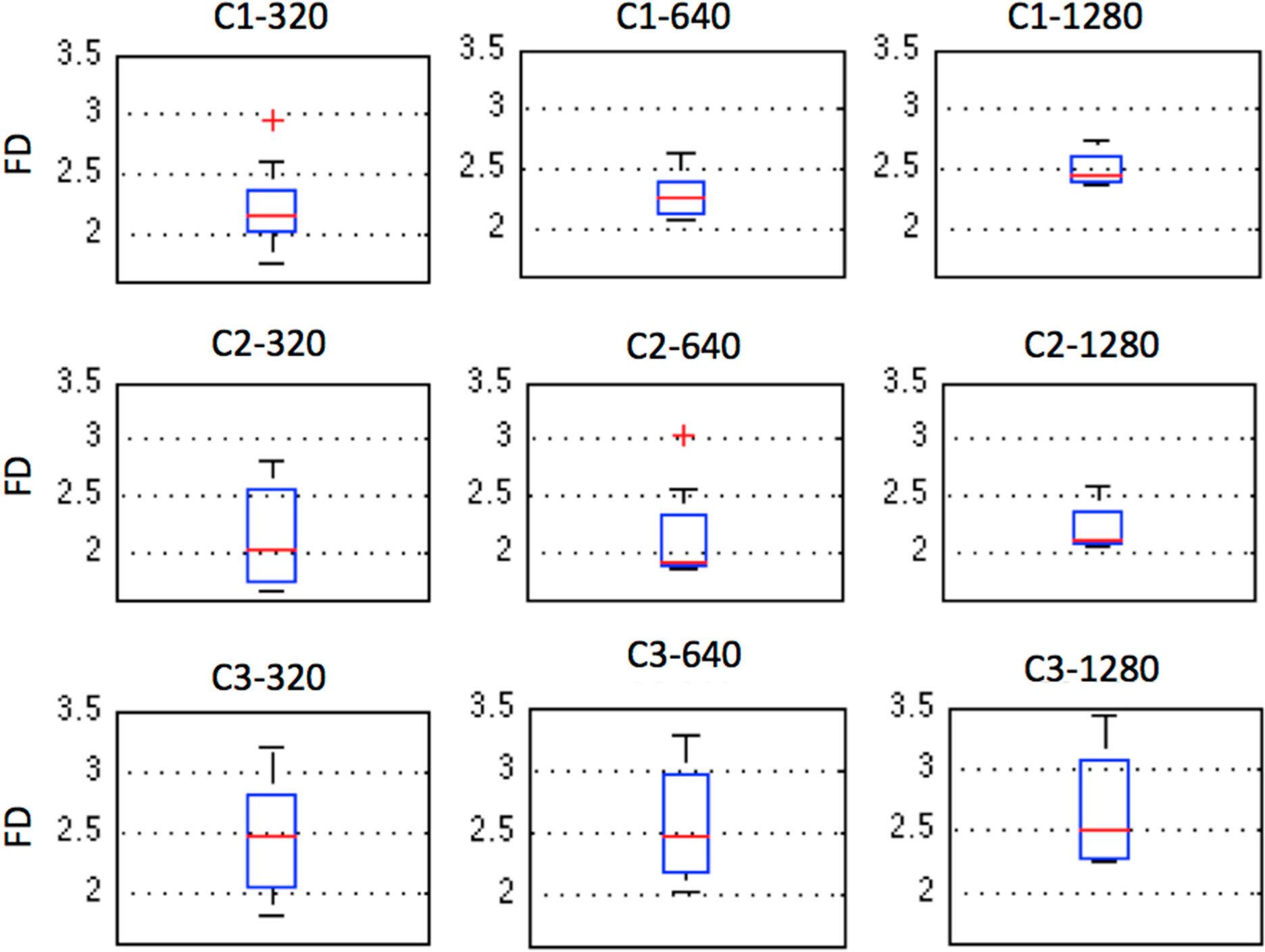
The median and the standard deviation of the FDs obtained for each case and window length for the Katz-Castiglioni algorithm on the X values are plotted in Figure 6 and shown in

Table 2. Medians of the Fractal Dimensions Obtained for Each Sliding Window Lenght (320, 640 and 1280) in C1, C2, and C3. Note how close are the medians for C3.

Case	Sliding Window Length
	320	640	1280
C1	2.1415	2.2624	2.4420
C2	2.0449	1.9188	2.1043
C3	2.4752	2.4618	2.5207

. C3 showed the highest FD median value for all three window lengths, with very similar values that were close to 2.5 (Table 2) but it also displayed the largest dispersion of values (Figure 6). C1 had the smallest dispersion of values (Figure 6) and they had a tendency to increase with increasing window length. The FD of C2 varied between 1.9 and 2.1. Increasing window length seemed to diminish the dispersion of the values in C1 and C2, but did not affect the degree of dispersion in C3 (Figure 6). Interestingly our results agree with those of [16] in spite of these authors using a different species (zebrafish, which is a freshwater species that prefers warmer water), only one individual and a different contaminant: the FD of the swimming trajectory of their zebrafish also trended to increasing concentrations of sodium hypochlorite contaminating its water, obtaining FD values of the swimming trajectories between 2.11 and 2.14. The value of the FD varies depending on the algorithm used for its calculation, on the different units composing the time series whether normalization has taken place or not as adressed by Fuss [65] and on the window length; with lower values of window length producing lower FD values. Optimization of the window length for our particular case produced FD values higher than 2, which is also in accordance with the results of Nimkerdphol and Nakagawa [16].

The Shannon Entropy values calculated on the same data as the FDs, i.e., the trajectories displayed in Figure 4 are shown in

Table 3. Shannon Entropy Values Calculated for the X and Y Coordinates for C1, C2, and C3.

Case	Shannon Entropy Values		Permutation Entropy Values
	X Coordinate	Y Coordinate	X Coordinate	Y Coordinate
C1	6.3016	6.3016	3.0881	3.0950
C2	6.2861	6.2861	3.1049	3.1250
C3	5.3628	5.3628	3.0413	3.0618

. There was no difference between the entropy calculated on the X or the Y values. It is noteworthy the large difference between the entropy of C3 and those of C1 or C2, which only differed slightly from each other (Table 3). This seems to indicate that the Shannon entropy decreases with increasing perturbation of the fish: tagging having only a minimal and possibly non-significant effect, but the presence of the contaminant drastically diminished the entropy of the system by an entire unit.

The permutation Entropy values calculated for the three experimental cases are also shown in Table 3. The results differ very slightly for X and Y signals and, in contrast to the results obtained using Shannon Entropy, the three analysed cases presented very similar permutation entropy values, although, in agreement with it, the permutation entropy values for C3 were smaller than for C1 and C2.

Technically, the method presented here demands a relatively large computation capability, particularly for the image processing step, which is of course susceptible of improvement. It must also be kept in mind on one hand that the analysis of the fish clusters trajectories does not depend on an image, they can also be obtained from echo-sounds or infrared images and, on the other hand, that the methodology is not exclusive for fish and that with some modification may be applicable to other species.

Of the tested methodologies, two of them, namely those based on the analysis of the Katz-Castiglioni FD and the Shannon entropy of the trajectories have been shown to be useful tools for non-invasive identification and quantification of changes of fish responses due to a highly relevant environmental contaminant. We believe that it will be possible to embed this methodology in an on-line/real time architecture to monitor fish schools in a farm and in the wild, and that this kind of approach will find an application to identify contaminated waters in environmental monitoring programs.

4. Conclusions and Future Work

In conclusion, the present work describes a method for image acquisition, processing and nonlinear trajectory analysis suitable to identify variations in the response to an event of fish groups. The methodology here proposed shows a clear potential to aid implementing intelligent aquaculture systems but it needs to be tested with more contaminants, stressors, fish species and validated, prior to be embedded in real-time automatic systems using artificial intelligence methods.