1. Introduction
Since the pioneering work on Hopfield neural networks was reported in [
1], the investigation of the dynamics of neurons has been receiving a lot of attention. In cellular neural networks [
2], Petráš pointed out that fractional derivatives instead of the integer order one were a natural choice. Recently, the utilities of fractional-order neural networks have been extensively studied, since the networks provide neurons with a fundamental and general computation ability that can contribute to efficient information processing, stimulus anticipation and frequency-independent phase shifts of oscillatory neuronal firing [
3]. It is well known that the uncertainty and time delay are unavoidable in many practical situations. For example, due to the finite switching speed of amplifier circuits in neural networks or dealing with motion-related problems, time delays exist in the information processing of neurons [
4]. On the other hand, most studies have been available under the assumption that the system parameters are assumed to be known in advance. However, under some circumstances, it is difficult to determine the values of parameters. Therefore, the fractional neural networks with unknown parameters and time delay are more general and reasonable in the real world.
If the parameters and time delays are appropriately chosen, the neural networks can exhibit complicated behaviors even with strange chaotic attractors. Meanwhile, synchronization of coupled neural networks has been investigated due to its potential applications in various engineering, including chaos generators design, secure communications, chemical and biological systems, information processing, distributed computation, optics, social science, harmonic oscillation generation, human heartbeat regulation and power system protection (see, e.g., [
4–
11] and the references therein). However, there are very limited results on the synchronization of fractional-order neural networks.
In this paper, an identification method based on fractional adaptive synchronization is applied to parameter identification of fractional-order neural networks with time delays. Fractional adaptive synchronization was a generalization of the integer case [
12,
13]. The main contributions of this paper mainly include three aspects: (i) An adaptive controller is first proposed, which is more general than the nonlinear controller [
14–
16]. Furthermore, the adaptive controller can be used to identify the unknown parameters of nonlinear part, but the nonlinear one may not. (ii) Our model of fractional neural networks with time delays and unknown parameters is more general. (iii) Based on a novel Lyapunov-like function and the Gronwall–Bellman integral inequality, we derive synchronization criteria analytically.
As mentioned above, fractional-order neural networks are very effective at applications due to their infinite memory. Besides, the fractional-order parameter and time delays enrich the system performance by increasing freedom. Synchronization of fractional neural networks with time delays may be more useful in many applications, such as information, pattern recognition and image processing. Therefore, it is necessary and interesting to study time-delayed fractional neural networks both in theory and in applications. The outline of the paper is organized as follows: some preliminaries and fractional-order neural networks are introduced in Section 2. The adaptive controller is proposed for two coupling networks, such that they can be synchronized in the following section. Numerical experiments are presented to support the theoretical analysis in Section 4. The conclusions are given in the last section.
2. Preliminaries and Model Description
In the following, we introduce some basic definitions and the corresponding results, which will be used later on.
Definition 1 ([
17]).
The fractional integral of order α for function f is defined as:where t ≥
t0,
α > 0
and Γ(·)
is the Gamma function. Definition 2 ([
17]).
The α-th-order Caputo fractional derivative of the given function f(
t)
is defined as: In most situations, the initial time t0 is often set to zero. Throughout the paper, t0 = 0 and
is simply denoted by Iα and
by Dα for brevity.
Lemma 1 ([
18]).
If x(
t) ∈
C1[0,
b]
and 0 <
α < 1,
then: Lemma 2 ([
19]).
Assume that x(
t) ∈
C1[0,
b]
and satisfies:for all t ∈ [0,
b],
then x(
t)
is monotonously non-decreasing. Ifthen x(
t)
is monotonously non-increasing. Lemma 3 ([
20]).
Let x(
t) ∈ ℝ
be a continuous and differentiable function. Then, for any time instant t ≥ 0
: Lemma 4 ([
21]).
For the given vectors x, y and a positive definite matrix Q > 0
with compatible dimensions, the following inequality holds,
Lemma 5 (Gronwall–Bellman integral inequality [
22]).
If z(
t)
satisfies with a(
t)
and b(
t)
being known real functions, thenIf b(
t)
is differentiable, thenIn particular, if b(
t)
is a constant, it immediately follows that We study the following drive and response fractional neural networks with time delays:
Here, 0 < α < 1,
i = 1, 2,⋯,
m;
xi(
t) denotes the state variable of the
i-th neuron at time
t;
aij and
bij denote the connection strengths and the time delay connection strengths, respectively;
âij and
are the estimations for the unknown connection strengths
aij and
bij;
fj(
xj(
t)),
gj(
xj(
t)) denote the activation functions of neurons;
τ is the time delay;
Ii is the input;
ui(
t) is a controller.
Hereafter, suppose that the activation functions
fi(
u) and
gi(
u) satisfy the Lipschitz conditions; that is, there exist constants
Fi > 0,
Gi > 0, such that:
for
u,
v ∈ ℝ and
i = 1, 2,⋯,
m.
3. Adaptive Controller for Uncertain Fractional-Order Neural Networks
In this section, we study the adaptive synchronization of two coupled fractional neural networks with unknown parameters. By the adaptive control theory, a simple controller for synchronization is designed and parameters identification is realized.
Let
ei(
t) =
yi(
t) −
xi(
t) and
e(
t) =
y(
t) −
x(
t) = (
e1(
t),
e2(
t),⋯,
em(
t))
T. Our goal is to design controller
u, such that the trajectory of the response system (
6) with initial condition
y0 can asymptotically approach that of the drive system (
5) with initial condition
x0 and, finally, implement synchronization, in the sense that:
where ║·║ is the Euclidean norm.
Theorem 1. The drive and response complex networks (5) and (6) can achieve synchronization, if the controller and the adaptive laws of parameters are taken as:where qij,
rij,
λi are arbitrary positive constants and the feedback strength ki(
t)
is adapted according to the following update law: Proof. From networks (
5) and (
6), one can get the following error system:
Now, we introduce the following Lyapunov-like function for system (
11):
where
ρi > 0,
i = 1, 2,⋯,
m and P is a semi-positive definite matrix under determination.
Define:
Applying
Equation (3) to (
13) yields:
By Lemma 2, we have that
w(
t) is monotonously non-decreasing,
i.e.,
w(
t) ≥
w(
t −
τ). Therefore,
V (
t) ≥ 0.
From Lemma 3,
Equations (9)–(
11), the fractional derivatives of
V (
t) along the solution can be derived as:
It immediately follows from (
14) that:
Here,
C =
diag(
c1,
c2,⋯,
cm) and
ρ =
diag(
ρ1,
ρ2,⋯,
ρm) are diagonal matrices;
A = (
aij)
n×n,
B = (
bij)
n×n are the connection matrices, and:
From Lemma 4 and assumption (
7), we can get the following two inequalities:
and:
where
F =
diag(
F1,
F2,⋯,
Fm) and
G =
diag(
G1,
G2,⋯,
Gm).
It follows from
Equations (16) and (
17) that:
Let:
Then, one has:
After fractional integration on both sides of the inequality (
18), we have:
Using
Equation (4) leads to:
Additionally,
eT (
t)
e(
t) ≤
V (
t) gives:
By Lemma 5, one has:
Therefore,
e(
t) → 0 as
t → ∞. □
Remark 1. It should be noted that Theorem 1 only derives the local stability of the fractional error system (11). In order to successfully identify the unknown parameters, other conditions must be satisfied. When achieving the synchronization, i.e., yi(
t) =
xi(
t),
as t → ∞,
error system (11) can be simplified as follows:According to the linear independence [
23],
the correct identification of the unknown parameters âij,
is equivalent to the fact that the function elements {
fj(
xj(
t)),
gj(
xj(
t−
τ)),
j = 1, 2,…,
m}
are linearly independent. Remark 2. Assume âij =
aij,
.
The system (5) and (6) can be asymptotically synchronized under the following control strategy:where λ
i > 0.
Remark 3. Assume.
The complete synchronization between system (5) and system (6) can be realized via the following control strategy:where qij,
λi are positive. 4. Numerical Simulation
4.1. Synchronization and Parameter Identification
In this section, numerical experiments are displayed to illustrate the effectiveness of the proposed method.
A group of fractional-order neural networks with time delay is considered, whose integer-order case was reported in [
10],
where:
The initial conditions for fractional neural networks (
19) are given as follows:
When we choose:
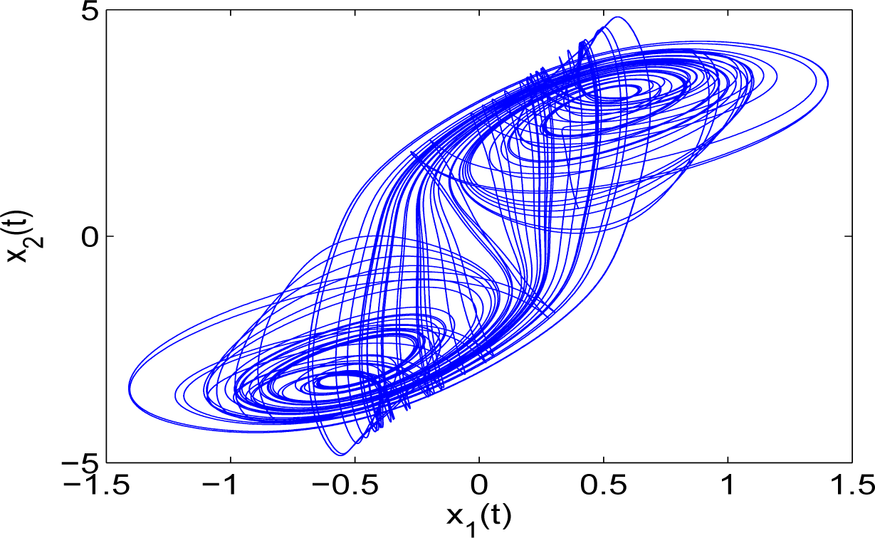
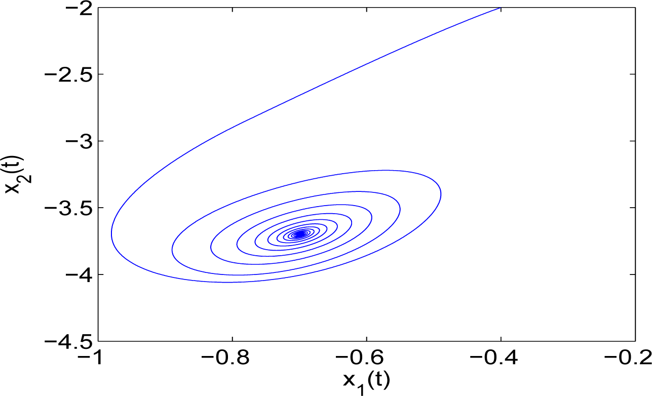
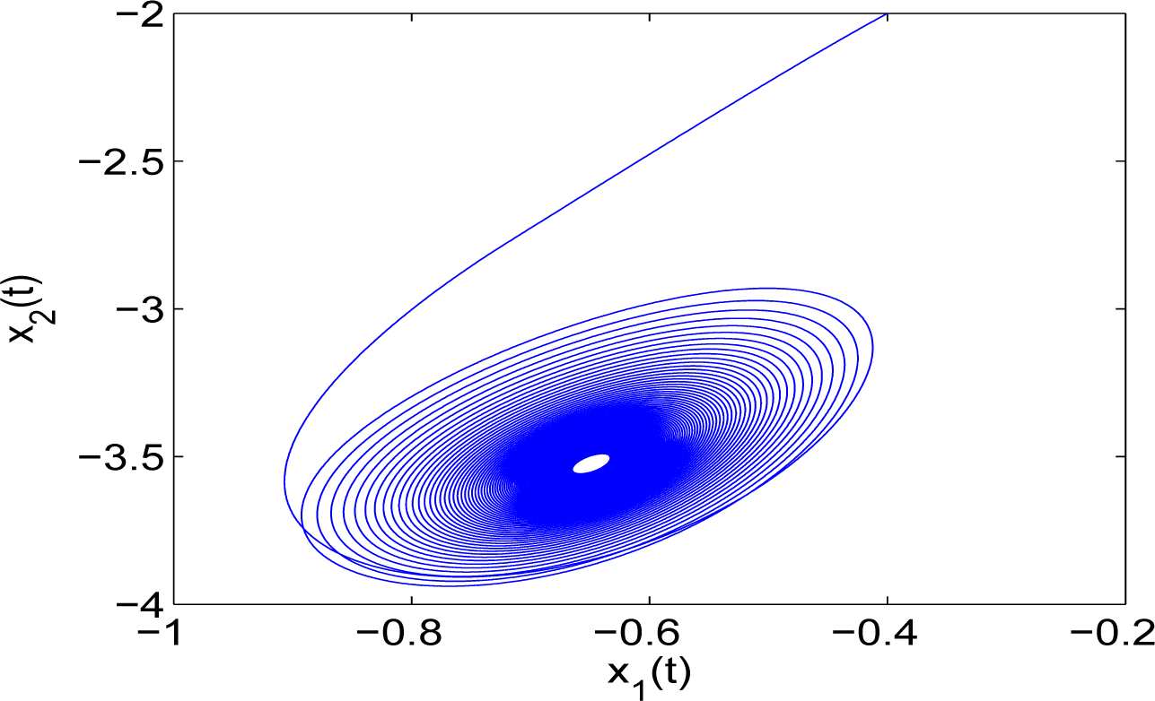
and A in the following three forms:
fractional system (
19) is chaotic (corresponding to A
1, see
Figure 1), has asymptotically stable equilibrium (corresponding to
A2, see
Figure 2), and has stable periodic solution (corresponding to
A3, see
Figure 3), respectively.
In the numerical simulations, the initial conditions and parameter values are given in the following:
Now, we choose
A =
A1,
qij = 5,
rij = 5 and λ
1 = λ
2 = 5 for the synchronization test.
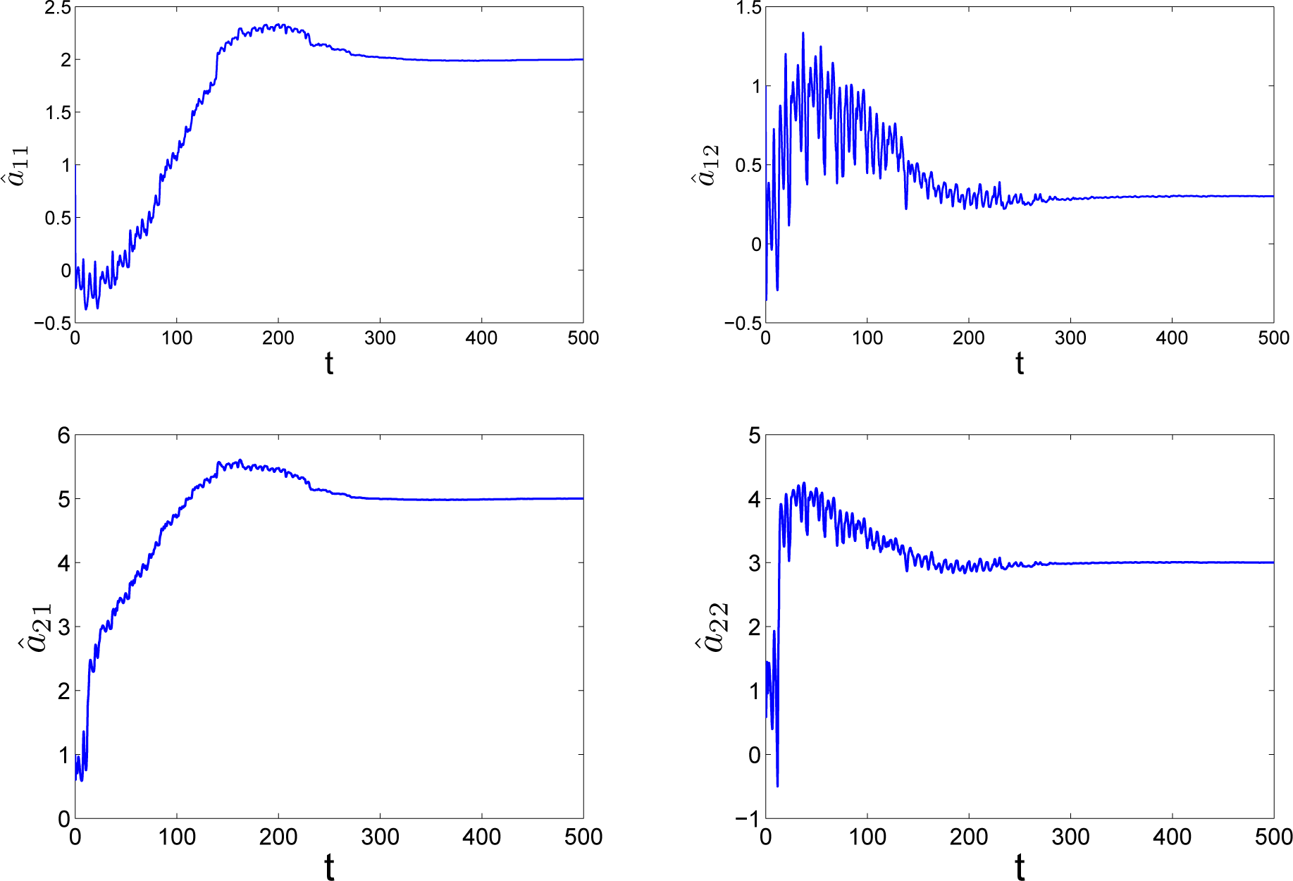
In the following, the adaptive control strategy (
9) and (
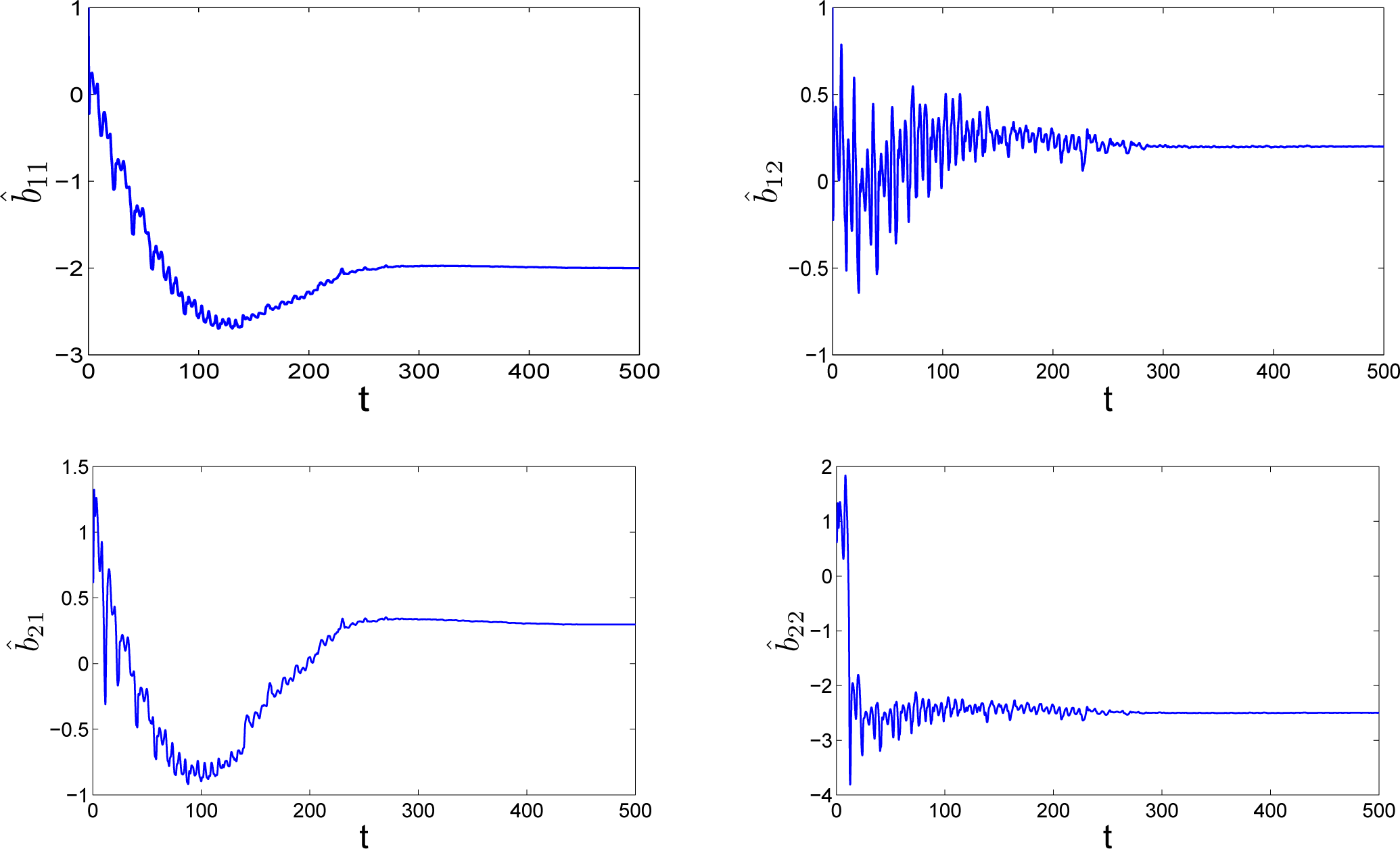
10) is used to identify the uncertain system parameters. From
Figures 4 and
5, it can be clearly seen that all the unknown system parameters
âij and
are successfully identified, respectively.
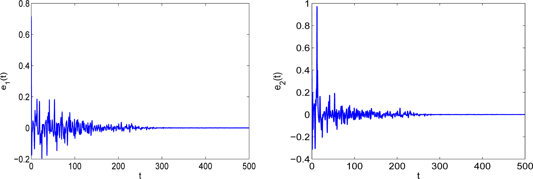
Figure 6 shows that the synchronization error converges to zero asymptotically. From
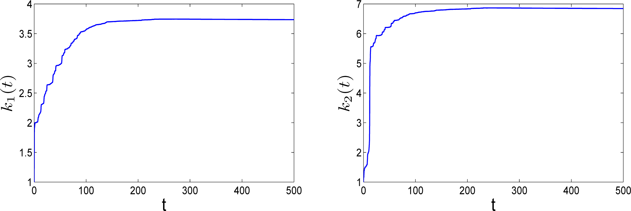
Figure 7, we can see that the adaptive control gains
ki(
t),
i = 1, 2 tend to some positive constants when system (
5) and system (
6) are synchronized.
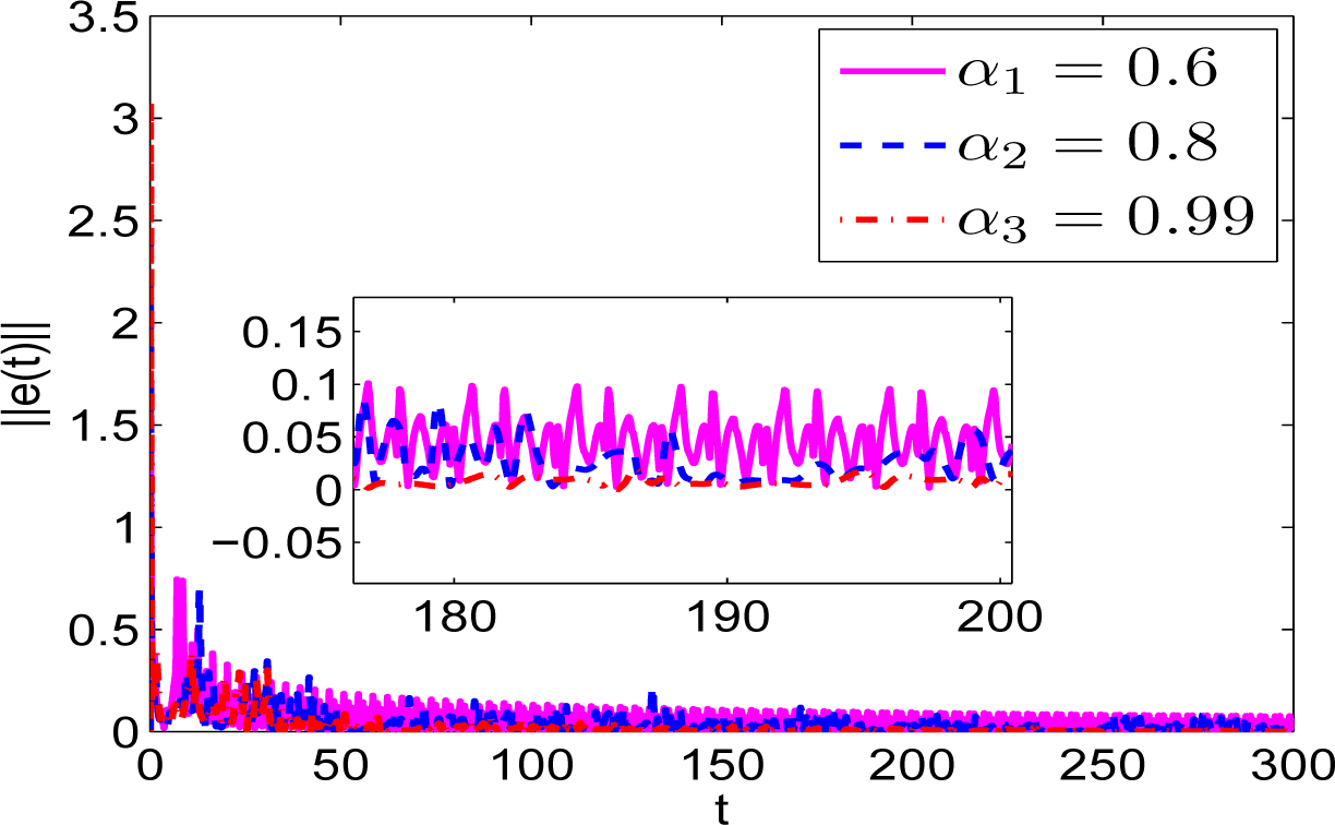
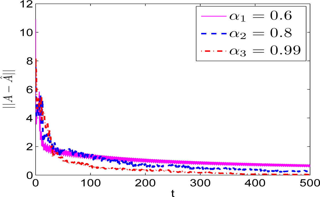
4.2. The Impact of Fractional Order on the Identification Process
The fractional order
αi has a direct effect on the chaotic behavior of the nonlinear dynamical systems. As a result, it also affects the synchronization behavior of fractional system. Bhalekar
et al. observed that the synchronization error decreases as the order
α increases [
12,
24]. However, the opposite phenomenon is also observed in [
25]. In this section, a more visible method is used to examine its impact on the fractional order neural networks with unknown parameters and time delays.
In order to numerically examine and avoid the linear dependence of the related functions [
12,
26], we let
α1 = 0.6,
α2 = 0.8,
α3 = 0.99. All of the other settings remain unchanged as stated in Section 4.1. From
Figures 8 and
10, we can obtain that the small value of the fractional order
αi would be harmful not only for synchronization state, but also for identification of unknown parameters for fractional neural networks.
5. Conclusions
In this paper, the identification of parameters and synchronization of fractional-order neural networks with time delays were studied. Especially, our designed adaptive controllers for network synchronization are rather simple in form. Moreover, the method discussed in this work can be well applied to other fractional-order complex networks with time delays.
Acknowledgments
This work was supported by the National Natural Science Foundation of China (Grant Nos. 11471150, 11372170, 61304173 and 41465002), the China Postdoctoral Science Foundation (Grant No. 2013M531107), the Foundation of Liaoning Educational Committee (Grant No. 13-1069) and the Fundamental Research Funds for the Central Universities (Grant No. 31920130003).
Author Contributions
In this paper, Weiyuan Ma was in charge of the control theory and adaptive synchronization design. Changpin Li was in charge of the fractional calculus theory and paper writing. Yujiang Wu and Yongqing Wu were in charge of the discussion and the simulation. All authors have read and approved the final manuscript.
Conflicts of Interest
The authors declare no conflict of interest.
References
- Hopfield, J.J. Neural networks and physical systems with emergent collective computational abilities. Proc. Natl. Acad. Sci. USA 1982, 79, 2554–2558. [Google Scholar]
- Petráš, I. A note on the fractional-order cellular neural networks. Proceedings of International Joint Conference on Neural Networks, Vancouver, BC, Canada, 16–21 July 2006; pp. 1021–1024.
- Lundstrom, B.; Higgs, M.; Spain, W.; Fairhall, A. Fractional differentiation by neocortical pyramidal neurons. Nat. Neurosci 2008, 11, 1335–1342. [Google Scholar]
- Gan, Q. Adaptive synchronization of Cohen–Grossberg neural networks with unknown parameters and mixed time-varying delays. Commun. Nonlinear Sci. Numer. Simul 2012, 17, 3040–3049. [Google Scholar]
- Gan, Q.; Xu, R.; Kang, X. Synchronization of unknown chaotic delayed competitive neural networks with different time scales based on adaptive control and parameter identification. Nonlinear Dyn 2012, 67, 1893–1902. [Google Scholar]
- Liao, T.L.; Tsai, S.H. Adaptive synchronization of chaotic systems and its application to secure communications. Chaos Solitons Fractals 2000, 11, 1387–1396. [Google Scholar]
- Song, Q. Design of controller on synchronization of chaotic neural networks with mixed timevarying delays. Neurocomputing 2009, 72, 13–15. [Google Scholar]
- Chen, G.; Zhou, J.; Liu, Z. Global synchronization of coupled delayed neural networks and applications to chaotic CNN models. Int. J. Bifurc. Chaos 2004, 14, 2229–2240. [Google Scholar]
- Gan, Q.; Dong, J.; Wu, M. Exponential synchronization for reaction-diffusion neural networks with mixed time-varying delays via periodically intermittent control. Neurocomputing 2014, 9, 1–25. [Google Scholar]
- Wang, K.; Teng, Z.; Jiang, H. Adaptive synchronization of neural networks with time-varying delay and distributed delay. Physica A 2008, 387, 631–642. [Google Scholar]
- Gan, Q.; Hu, R.; Liang, Y. Adaptive synchronization for stochastic competitive neural networks with mixed time-varying delays. Commun. Nonlinear Sci. Numer. Simul 2012, 17, 3708–3718. [Google Scholar]
- Si, G.; Sun, Z.; Zhang, H.; Zhang, Y. Parameter estimation and topology identification of uncertain fractional order complex networks. Commun. Nonlinear Sci. Numer. Simul 2012, 17, 5158–5171. [Google Scholar]
- Yang, L.; Jiang, J. Adaptive synchronization of driver-response fractional-order complex dynamical networks with uncertain parameters. Commun. Nonlinear Sci. Numer. Simul 2014, 19, 1496–1506. [Google Scholar]
- Wu, X.; Lu, H.; Shen, S. Synchronization of a new fractional-order hyperchaotic system. Phys. Lett. A 2009, 373, 2329–2337. [Google Scholar]
- Yang, L.; Jiang, J. Hybrid projective synchronization of fractional-order chaotic systems with time delay. Discret. Dyn. Nat. Soc 2013, 2013, 459801. [Google Scholar]
- Wang, S.; Yu, Y.; Wen, G. Hybrid projective synchronization of time-delayed fractional order chaotic systems. Nonlinear Anal. Hybrid Syst 2014, 11, 129–138. [Google Scholar]
- Podlubny, I. Fractional Differential Equations: An Introduction to Fractional Derivatives, Fractional Differential Equations, Some Methods of Their Solution and Some of Their Applications; Academic Press: San Diego, CA, USA, 1999. [Google Scholar]
- Li, C.; Deng, W. Remarks on fractional derivative. Appl. Math. Comput 2007, 187, 777–784. [Google Scholar]
- Yu, J.; Hua, C.; Jiang, H.; Fan, X. Projective synchronization for fractional neural networks. Neural Netw 2014, 49, 87–95. [Google Scholar]
- Aguila-Camacho, N.; Duarte-Mermoud, M.A.; Gallegos, J.A. Lyapunov functions for fractional order systems. Commun. Nonlinear Sci. Numer. Simul 2014, 19, 2951–2957. [Google Scholar]
- Boyd, S.; EI Ghaoui, L.; Feron, E.; Balakrishnan, V. Linear Matrix Inequalities in System and Control Theory; SIAM: Philadelphia, PA, USA, 1994. [Google Scholar]
- Slotine, J.J.E.; Li, W.P. Applied Nonlinear Control; Prentice Hall: Englewood Cliffs, NJ, USA, 1991. [Google Scholar]
- Andrilli, S.; Hecker, D. Elementary Linear Algebra, 4th ed.; Academic Press: Burlington, MA, USA, 2010. [Google Scholar]
- Bhalekar, S.; Daftardar-Gejji, V. Synchronization of different fractional order chaotic systems using active control. Commun. Nonlinear Sci. Numer. Simul 2010, 15, 3536–3546. [Google Scholar]
- Wu, X.; Lai, D.; Lu, H. Generalized synchronization of the fractional-order chaos in weighted complex dynamical networks with nonidentical nodes. Nonlinear Dyn 2012, 69, 667–683. [Google Scholar]
- Tavazoei, M.S.; Haeri, M. Chaotic attractors in incommensurate fractional order systems. Physica D 2008, 237, 2628–2637. [Google Scholar]
© 2014 by the authors; licensee MDPI, Basel, Switzerland This article is an open access article distributed under the terms and conditions of the Creative Commons Attribution license (http://creativecommons.org/licenses/by/4.0/).


