Autonomous Search for a Diffusive Source in an Unknown Structured Environment

Abstract

The paper presents a framework for autonomous search for a diffusive emitting source of a tracer (e.g., aerosol, gas) in an environment with an unknown map of randomly placed and shaped obstacles. The measurements of the tracer concentration are sporadic, noisy and without directional information. The search domain is discretised and modelled by a finite two-dimensional lattice. The links in the lattice represent the traversable paths for emitted particles and for the searcher. A missing link in the lattice indicates a blocked path due to an obstacle. The searcher must simultaneously estimate the source parameters, the map of the search domain and its own location within the map. The solution is formulated in the sequential Bayesian framework and implemented as a Rao-Blackwellised particle filter with entropy-reduction motion control. The numerical results demonstrate the concept and its performance.

1. Introduction

The search for an emitting source of particles, chemicals, odour or radiation, based on sporadic clues or intermittent measurements, has attracted a great deal of interest lately. In the biological context, the search is studied to understand animal behaviour in the search for food or mates [1–3], to model the biochemical reactions in cells (the search for specific DNA sequences by transcription factors [2,4], genetic-based therapy [5]) and to simulate intracellular transport (viral trafficking in a microtubule network [6,7]).

Industrial applications mainly focus on rescue operations with the goal of localising hazardous pollutants, such as chemical leaks [8–10] or radioactive sources [11–13]. The search strategies can be broadly divided into two categories. The first includes conventional methods, which are guided by the positive concentration gradient (“chemotaxis”) [14] and its variants [15]. Vergassola et al. [16] formulated another search strategy (referred to as “infotaxis”), which is driven by the information gain or entropy-reduction (for a comprehensive review, see [17]).Information-gain guided searchhas been successfully applied in the context of finding a weak source in a turbulent flow (e.g., drug or leak emitting chemicals [16,17])and localising radioactive point sources [12,13].The crucial advantage of “infotaxis” versus “chemotaxis” is that the former can be used even when the estimation of concentration gradient is infeasible, which is always the case in the presence of sporadic or intermittent measurements.

While all works referenced above deal with search in an open domain (without obstacles) or assuming that a precise map of the search domain (with obstacles) is a priori available, in this paper, we focus on autonomous search for a diffusive emitting source in a domain with randomly placed and shaped obstacles (forbidden areas), whose structure (the map) is unknown. The problem is of importance, for example, in the localisation of dangerous leaks in collapsed buildings, inside tunnels or mines. The searcher senses in a probabilistic manner both the structure of the search domain (e.g., the presence or absence of obstacles, walls, blocked passages) and the level of concentration of tracer particles. The objective of the search is to navigate through the unknown environment for the purpose of source localisation in the shortest possible time. Once the source is localised, the coordinates of the source relative to its starting position (or the path to the source) need to be reported.

This is not a trivial task for several reasons. First, the measurements of the tracer particle concentration are sporadic, noisy and without directional information. Furthermore, the emission rate of the source is typically unknown (hence, the concentration measurement cannot easily be related to the distance between the source and the searcher). Finally, the searcher needs to explore the domain, create its partial map (which must include the starting point and the source) and localise itself relative to this map. This partial map is important, for example, in order to guide the rescue team to the source or to help the searcher retreat to its starting position (simple obstacle avoidance methods clearly would be insufficient for this purpose). Among the search schemes that are intended to deal with the sporadic measurements and that directly address the balance between exploitation of the information accumulated during the search and exploration of the environment, “infotaxis” is the most efficient, exhibiting the lowest average search time and the highest reliability in source reaching [18]. For this reason, we adopt an information-driven search strategy in the paper.

The searcher operates in a fully autonomous manner: it senses the environment (the concentration of a tracer; the position of obstacles) and after processing the sensor data (which is inherently uncertain, due to the noise in perception and actuation), it subsequently makes a decision on where to move next in order to collect new measurements. Its motion control is not noise-free, as it may occasionally fail to execute correctly. Hence, the searcher unknowingly may move to a position different from intended. The probabilistic models of searcher motion and sensor measurements is assumed to be known.

In the paper, we consider a two-dimensional search domain. The coordinates of the initial position of the searcher, as well as the border of the search area (relative to the initial position) are given as input parameters. In order to fulfil its mission (i.e., find the source and report its coordinates relative to its starting position), the searcher must carry out simultaneous estimation at three levels: (1) estimation of source parameters (its location in 2D and its release rate); (2) estimation of the map of the search area; and (3) estimation of the searcher position within the estimated map. Estimation at levels (2) and (3) has been studied extensively in robotics under the term grid-based simultaneous localisation and mapping (SLAM) [19]. The primary mission in all SLAM publications is an accurate mapping of the area. The primary mission of our searcher, however, is to localise the source, while SLAM is only a necessary component of the solution.

The search domain is discretised, as, for example, in [8], and modelled by a finite two-dimensional lattice. With a sufficiently fine resolution of the lattice, the emitting source can be considered to be in one of the nodes of the lattice. The links (edges) of the lattice represent the traversable paths for emitted particles (tracer) and for the searcher. Missing links in the lattice indicate blocked paths due to walls or obstacles. This is a very general model applicable to searches at various scales, from inside buildings and tunnels, to within cells of living organisms [2]. The percentage of missing links in the lattice is assumed to be above the percolation threshold p_c (for the adopted lattice structure p_c = 1/2 [20,21]), so that long-range connectivity is satisfied [20]. Using the absorbing Markov chains technique [22], we can compute exactly the mean concentration level in any node of the lattice, that is, at any point of the search domain with obstacles.

Since the structure (map) of the search domain is unknown, the searcher must rely on a theoretical model of concentration measurement, which is independent of the map. An approximation of such a model is derived in an analytic form using conformal mapping [23].

The only related work that deals with autonomous search in an unknown structured environment is [24]. While [24] presents a plethora of interesting experimental results, the algorithms are based on heuristics. The contribution of our paper is a theoretically sound framework for autonomous search for a diffusive source in an unknown environment. The mathematical models of tracer distribution (for known and unknown maps), as well as the models of measurements and motion dynamics, are derived or precisely specified. Estimation of source parameters, the map and the searcher location within the map is carried out in the optimal sequential Bayesian framework, implemented using a Rao-Blackwellised particle filter. Finally, the searcher motion is driven by the maximisation of the information gain (i.e., entropy reduction), which, on average, results in the shortest average search time.

The paper is organised as follows. Mathematical models of tracer distribution, measurements and searcher motion are described in Section 2. The autonomous search problem is formulated and its conceptual solution provided in Section 3. Full technical details of the proposed search algorithm are presented in Section 4, with numerical results given in Section 5. Finally, conclusions of this study are summarised in Section 6.

2. Modelling

2.1. Model of the Environment

The concentration of a tracer at any point in the search domain is governed by the diffusive equation, which, in the steady state, reduces to the Laplace equation [25]:

$$D_0\Delta \theta =A_0\delta (x-X,y-Y).$$

(1)

Here, D₀ is the diffusion coefficient of tracer in the environment, Δ is the Laplace operator, θ is the mean (time-averaged) tracer concentration, δ is the Dirac delta function, A₀ is the release-rate of the tracer source and X, Y are the coordinates of the source in a two-dimensional Cartesian coordinate system. We remark here that D₀ is treated as an aggregated parameter, whose value approximately captures the main diffusion processes in the system. Depending on the problem context, this may be molecular diffusion, turbulent diffusion, flow-induced diffusion, confined (compartmented structure) diffusion, etc.

For convenience we adopt a circular search area of radius R₀, centred on the origin of the coordinate system, that is, for every point inside the search area, $r=\sqrt{x^2+y^2}\le R_0$. Assuming that the tracer source is undetectable outside the search domain, we can impose the absorbing boundary condition θ (r = R₀) = 0. The traditional approach to the computation of the tracer concentration, θ, at every point of the search domain is via analytical or numerical solution of Equation (1). This, however, is a nontrivial task when the search domain is a structure of complex topology (due to obstacles, compartments walls, random openings, etc.).

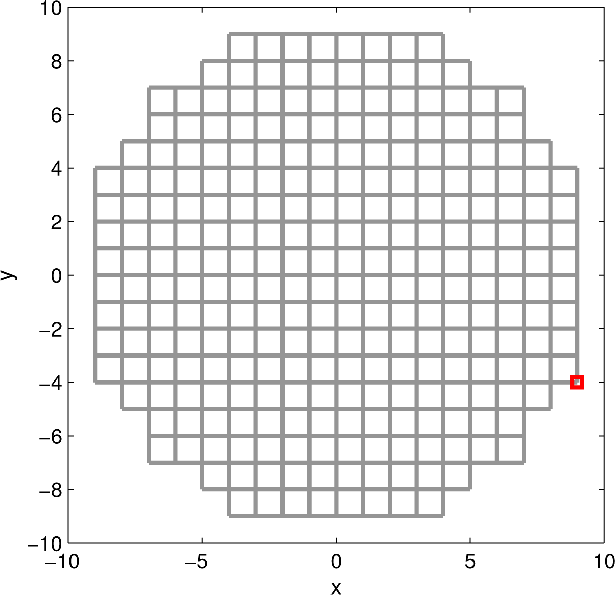
We therefore adopt an alternative approach, where the continuous model of the tracer diffusion process is replaced with a random walk on a square lattice, adopted as a discrete model of the search area. Discretisation is illustrated in Figure 1 for a search area centred on the origin of the coordinate system, with the radius R₀ = 9. The length of each link (edge, bond) in the lattice determines the resolution of discretisation and, in this example, is adopted as a unit length. The source, assumed to be located at one of the nodes of the lattice, is emitting particles that travel through the lattice according to the random walk model [26].

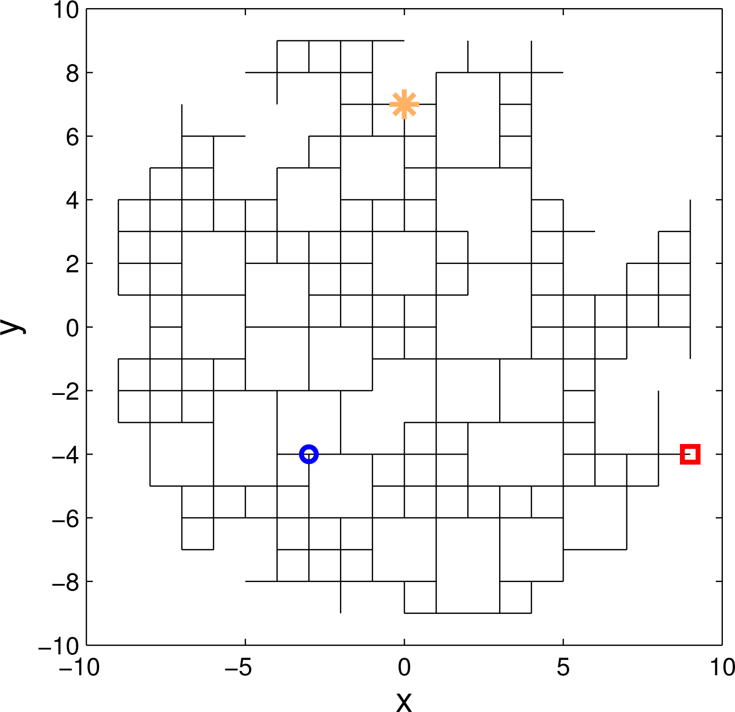
The obstacles in the search domain (the regions through which the tracer cannot pass) are simply modelled as missing links (or clusters of missing links) in the square lattice. Figure 2 shows an example of such a model: this incomplete lattice is obtained by removing fraction p ≈ 0.35 of the links in the complete lattice shown in Figure 1. Note that all nodes in the incomplete lattice are connected. On average, this will be the case if the fraction of missing links in the incomplete grid of Figure 2 is below the percolation threshold, p_c; above the percolation threshold (p > p_c), the lattice becomes fragmented. The framework of percolation theory enables the analytical description of statistical properties of such a lattice [20,21].

2.2. Model of Tracer Distribution

This section explains how to compute the mean concentration of tracer particles in each node of the incomplete grid (such as the one shown in Figure 2), which represents a discretised model of the search area with obstacles.

For a given incomplete grid, the mean concentration can be computed using the absorbing Markov chain technique [22]. Neglecting the spatial approximation of the search domain (due to discretisation) and under the assumption that the distribution of particles has reached the steady state, the absorbing Markov chain provides an exact solution for the quantity of source material at each location.

We can regard the random walk of tracer particles through the incomplete grid (e.g., Figure 2) as a Markov chain whose states are the nodes of the grid. The Markov chain is specified by the transition matrix, T; each element of this matrix is the probability of the transition from state s_i to state s_j (i.e., a particle move from node i to node j): T_ij = P {s_j|s_i}. How does one construct T given the incomplete grid? First note that we distinguish two types of states in this Markov chain: absorbing states (corresponding to the nodes on the boundary of the grid) and transient states. For an absorbing state, s_i, T_ii = 1 and T_ij = 0, if j ≠ i. Suppose a transient state, s_i, corresponds to node i in the incomplete grid, which has connections (links) with nodes j₁,…, j_m, where for a square grid m ≤ 4. Then, T_ij1 = · · · = T_ijm = 1/m and T_ij = 0 for j ∉ {j₁,…, j_m}.

Suppose there are r absorbing states and t transient states. If we order the states so that the absorbing states come first (before the transient states), then the transition matrix takes the canonical form:

$$\mathbf{T}=\left[\begin{array}{ll}{\mathbf{I}}_r\hfill & \mathbf{0}\hfill \\ \mathbf{R}\hfill & \mathbf{Q}\hfill \end{array}\right]$$

(2)

where I_n denotes the n × n identity matrix, Q is a t × t matrix that describes the transitions between the transient states, R is a t × r matrix that describes the transitions from the transient to absorbing states and 0 is an r × t matrix of zeros. The fundamental matrix of the absorbing Markov chain [22],

$$\mathbf{F}={({\mathbf{I}}_t-\mathbf{Q})}^{-1}$$

(3)

represents the probability of being in state s_j having started from a transient state, s_i (before being absorbed). This matrix hence can be used to compute the mean particle concentration in any node of the incomplete grid at steady state. Suppose an emitting source is placed at node i, which is not on the boundary. The source is releasing tracer particles at a constant rate, A₀. Then, the expected concentration of tracer particles in any other node, j, of the incomplete grid (which is not on the boundary) is given by θ_j = A₀ · F_ij. The concentration scales linearly with the release rate, A₀, which is a direct consequence of the linearity of Laplace Equation (1).

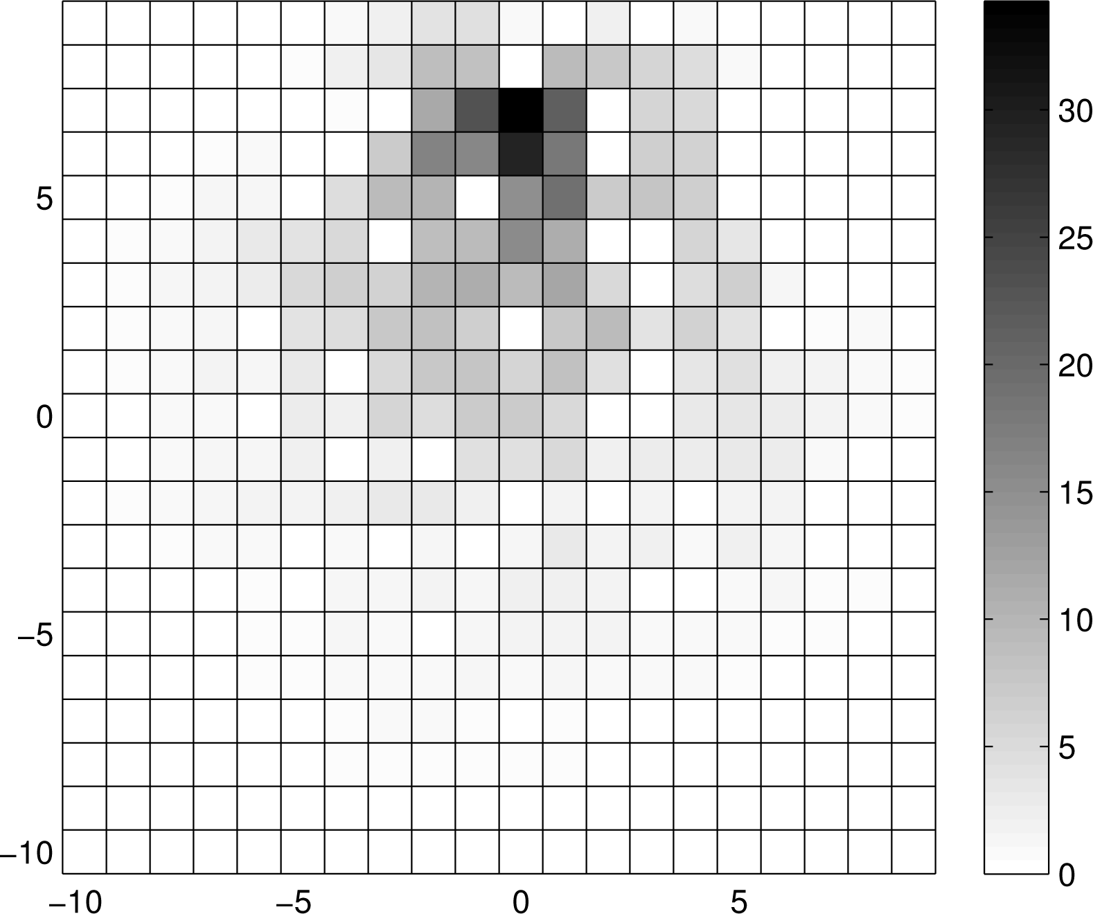
Figure 3 shows the mean concentration of tracer particles for the search area modelled by the incomplete grid of Figure 2, with the source placed at (X, Y) = (0, 7) and with A₀ = 12. Notice from Figure 3 how the concentration depends on the distance from the source and the structure of the grid, plotted in Figure 2.

2.3. Sensor Models and Motion Model

Two types of measurements are collected by the searcher. Sensor 1 measures the concentration of tracer particles as a count of particles received during the sampling interval. Assuming the so-called “dilution” limit (limit of low concentrations), the tracer fluctuations follow the Poisson distribution [16], that is, a concentration measurement at node j of the grid is a random sample drawn from

$$n~𝒫(n;\lambda )=\frac{{\lambda }^n}{n!}{e}^{-\lambda }$$

(4)

where λ= θ_j = A₀ · F_ij. The Poisson distribution mimics the intermittency of concentration measurements [16].

The searcher sequentially estimates the source parameters without knowing the map of the search area. Hence, the measurement model based on the mean concentration λ= A₀ · F_ij cannot be used in estimation (recall that matrix F is formed using knowledge of the structure of the incomplete lattice). Assuming that the fraction of missing links in the lattice is smaller than the percolation threshold, p_c, the expected concentration of tracer particles in any node, j, of the incomplete lattice can be computed approximately using the property of conformal invariance of the Laplace equation (see Appendix 6 for details). Suppose the source of release rate A₀ is placed at a node of the grid, positioned at coordinates (X, Y). Then, the mean (time and ensemble averaged) concentration at node j, positioned at (x_j, y_j), can be approximated as

$${\langle \theta \rangle }_j\approx -\frac{A}{2}\text{log}(R^2)$$

(5)

where A = A₀/f_c, (f_c is a constant, 0 < f_c < 1, which depends on the fraction of missing links in the incomplete grid (see Appendix 6)) and

$$R^2=R_0^2\frac{{(x_j-X)}^2+{(y_j-Y)}^2}{{(x_{j}Y-y_{j}X)}^2+{(R_0^2-x_{j}X-y_{j}Y)}^2}.$$

(6)

Note that this model is independent of the structure of the incomplete lattice. In summary, estimation will be carried out using Sensor 1 measurement model in Equation (4), where mean λ = 〈θ〉_j is approximated by Equations (5) and (6). The actual concentration measurements also follow the model in Equation (4), but with λ =θ_j = A₀ · F_ij. This is how we simulate measurements in Section 5.

The searcher moves and explores the search domain in order to find the source. The source parameter estimation is carried out using the map-independent measurement model in Equation (5), which does not require discretisation of the search domain on a square lattice (as in Figure 1). Nevertheless, we keep discretisation for the searcher in order to model its motion paths and to facilitate its grid-based SLAM functionality. Thus, we assume that the searcher travels within the search area along the paths represented by the links of the incomplete grid as in Figure 2. As it travels, it stops at the nodes along its path to sense the environment, i.e., to collect measurements.

Sensor 2 is a simple binary detector of the presence or absence of the links (paths) visible from the node in which the searcher is currently placed. It reports on the presence/absence of the primary and secondary neighbouring links.

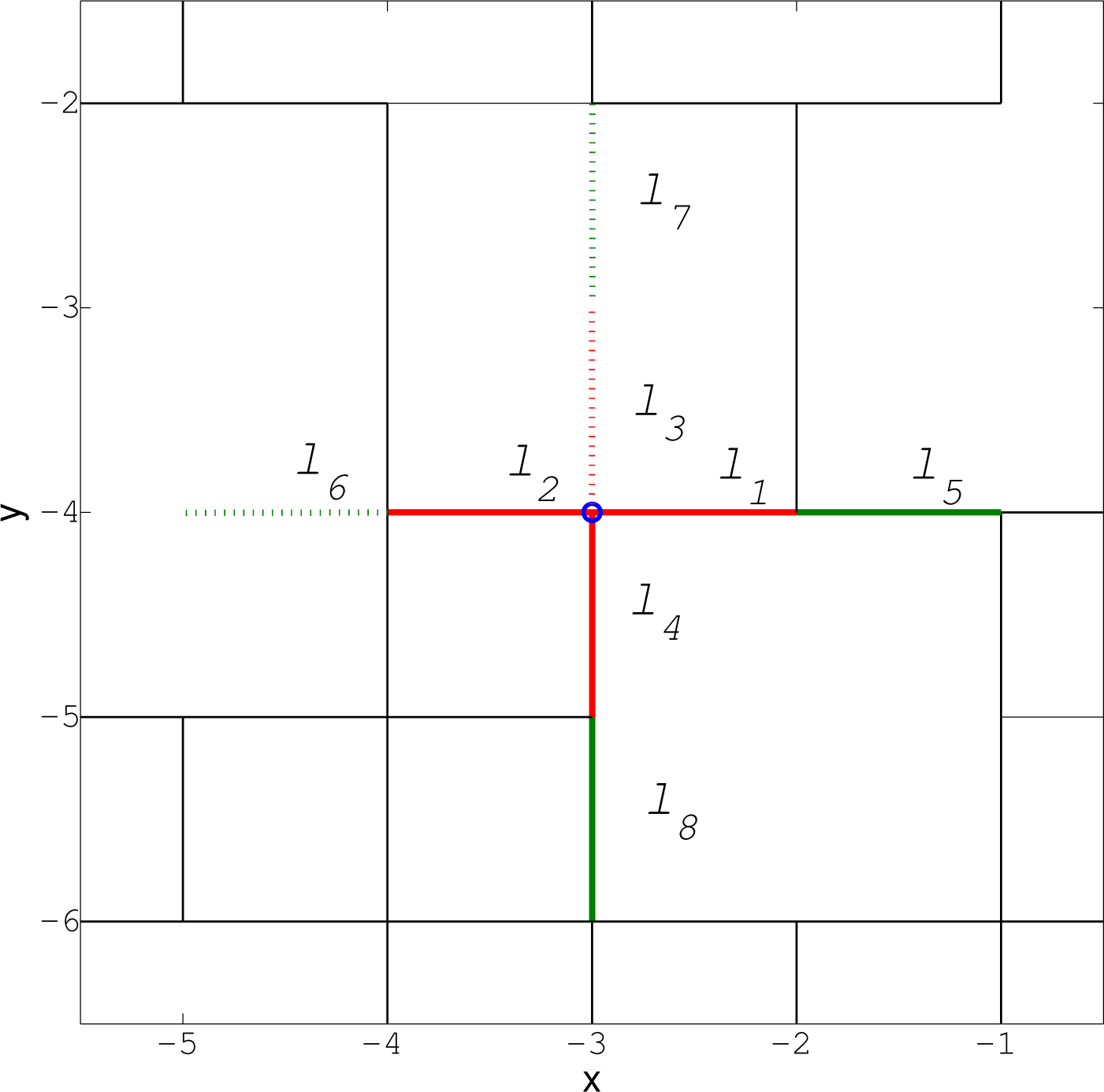
A link in a grid of Figure 2 is defined by a quadruple (x₁, y₁, x₂, y₂), where (x₁, y₁) and (x₂, y₂) are the coordinates of the nodes it connects. In order to explain what we mean by primary and secondary links, consider for example the node at location (−3, −4) indicated by “o” in Figure 2; the zoomed-in segment is shown in Figure 4. The primary links from this node are the connecting links towards east, west, up and down from (−3, −4), plotted in red in Figure 4; for example, ℓ₁ = (−3, −4, −2, −4). The status of a link, ℓ, denoted m(ℓ), is a binary variable with the convention that m(ℓ) = 1 means that the link ℓ exists. According to Figures 2 and 4, we have: m(ℓ₁) = 1, m(ℓ₂) = 1, m(ℓ₃) = 0, m(ℓ₄) = 1. Existing links are shown by solid lines in Figure 4, while non-existing links are plotted as dotted lines.

The secondary links from the node at (−3, −4) in Figure 2 represent second neighbouring links in direction of east, west, up and down from (−3, −4), that is, ℓ₅ = (−2, −4, −1, −4), and so on. According to Figures 2 and 4, the status of secondary links is: m(ℓ₅) = 1, m(ℓ₆) = 0, m(ℓ₇) = 0, m(ℓ₈) = 1; existing secondary links are indicated by solid green lines in Figure 4. A secondary link is observable if the connecting primary link to it exists in the graph. In Figures 2 and 4, for example, ℓ₅, ℓ₆ and ℓ₈ are observable, but ℓ₇ is not, because m(ℓ₃) = 0.

Let an observation (supplied by sensor 2) about the presence or absence of a link, ℓ, be a binary value z(ℓ) ∈{0, 1}, where z(ℓ) = 0 means link ℓ is absent and z(ℓ) = 1 is the opposite. The performance of sensor 2 can be described by two detection matrices, one for the primary links, the other for observable secondary links. Each detection matrix, П, has a form

$$\prod =\left[\begin{array}{cc}P(z=0|m=0)& P(z=0|m=1)\\ P(z=1|m=0)& P(z=1|m=1)\end{array}\right]$$

(7)

where P (z = 1|m = 1) = p_d and P (z = 1|m = 0) = p_fa are the probability of correct detection and the probability of false detection p_fa, respectively. The columns of matrix add up to one, and, hence, Equation (7) can be written as

$$\prod =\left[\begin{array}{cc}1-p_{fa}& 1-p_d\\ p_{fa}& p_d\end{array}\right]\cdot$$

(8)

Suppose the searcher is in node i at discrete time k − 1. Let the set of admissible controls vectors for the next move be defined as $𝒰$_k = {·,→, ←, ↑, ↓}, meaning that the searcher can stay where it is, or move one unit length to the right, to the left, up or down. After processing measurements from its sensors, the searcher decides to choose control ${\mathbf{u}}_k^{*}\in {𝒰}_k$ and, hence, to arrive at time k at node j. However, due to control noise or unmodelled exogenous effects [19], control ${\mathbf{u}}_k^{*}\in {𝒰}_k$ is executed correctly only with probability 1 − p_e; with probability p_e, the searcher will actually execute control ${u^{\prime }}_k\in {𝒰}_k\backslash \left\{{\mathbf{u}}_k^{*}\right\}$.

3. The Problem and Its Conceptual Solution

The searcher has at its disposal the probabilistic models of sensor measurements and dynamic models. Prior knowledge also includes: (1) the coordinates of its initial position; (2) the length of each link in the square lattice; and (3) the boundary of the circular search area (defined by its centre and radius). The described prior translates into knowledge of the full grid, such as the one shown in Figure 1. Searcher motion is restricted to this full grid.

The objective of the searcher is to estimate in the shortest possible time the coordinates of the emitting source, as well as the partial map describing the path from its starting (entry) point to the estimated location of the source.

3.1. Sequential Bayesian Estimation

The described problem can be cast in the sequential Bayesian estimation framework as a nonlinear filtering problem. Let us first define the state vector, which consists of three parts:

(1)

The coordinates of the searcher position at discrete time k = 1, 2, . . . are denoted by p_k = [x_k y_k]^т.

(2)

The status (presence/absence) of each link in the complete grid (such as the one shown in Figure 1). The status of link ℓ_j, where j = 1, . . . , L and L is the total number of links in the complete grid, is m(ℓ_j) = m_j ∈ {0, 1}. The notation P (m_j = 1) refers to the probability that link ℓ_j is present. The map at time k is fully specified by vector m_k = [m_1,k, . . . , m_L,k]^т. The time index is introduced, because we allow the map of the search area to occasionally change, e.g., an open door can close. The assumption is that the statuses of links are mutually independent, i.e., m_j,k is independent from m_i,k for i ≠ j.

(3)

The parameter vector of the source is denoted by s = [X Y A]^т.

The complete state vector is then defined as ${\mathbf{y}}_k={\left[{\mathbf{p}}_k^{⊺}\hspace{0.17em}\hspace{0.17em}{\mathbf{m}}_k^{⊺}\hspace{0.17em}\hspace{0.17em}\hspace{0.17em}{\mathbf{s}}^{⊺}\right]}^{⊺}$, where p_k and m_k are discrete state variables, while s is a continuous state vector. Dynamics of the state, y_k, are described by two transitional densities: p(m_k|m_k−1) specifies the evolution of the map over time, while p(p_k|p_k−1, u_k) characterises the searcher motion model. The observation models of the searcher are specified by two likelihood functions: g₁(n_k|p_k, m_k, s) characterises sensor 1, which provides the count of particles n_k at position p_k coming from the source in state s through the map m_k; g₂(z_k|p_k, m_k) refers to sensor 2 and describes the observation z_k of the status of the links in m_k visible from the searcher in location p_k. Let us denote observations at time k by a vector ${\zeta }_k={\left[n_k{z}_k^{⊺}\right]}^{⊺}$. Finally, the prior probability density function (pdf) of the state is denoted by p(y₀).

The goal in the sequential Bayesian framework is to estimate any subset or property of the sequence of states y_0:k := (y₀, . . . , y_k) given observation sequence ζ_1:k := (ζ₁, . . . , ζ_k) and the control sequence u_1:k := (u₁, . . . , u_k), which is completely specified by the joint posterior distribution p(y_0:k|ζ_1:k, u_1:k). This posterior satisfies the following recursion:

$$p({\mathbf{y}}_{0:k}|{\zeta }_{1:k},{\mathbf{u}}_{1:k})=\frac{g({\zeta }_k|{\mathbf{y}}_k)p({\mathbf{y}}_k|{\mathbf{y}}_{k-1},{\mathbf{u}}_k)}{p({\zeta }_k|{\zeta }_{1:k-1})}p({\mathbf{y}}_{0:k-1}|{\zeta }_{1:k-1},{\mathbf{u}}_{1:k-1})$$

(9)

where

$$p({\mathbf{y}}_k|{\mathbf{y}}_{k-1},{\mathbf{u}}_k)=p({\mathbf{m}}_k|{\mathbf{m}}_{k-1})p({\mathbf{p}}_k|{\mathbf{p}}_{k-1},{\mathbf{u}}_k)$$

(10)

is the transitional density, and

$$g({\zeta }_k|{\mathbf{y}}_k)=g_1(n_k|{\mathbf{p}}_k,{\mathbf{m}}_k,\mathbf{s})\hspace{0.17em} g_2({\mathbf{z}}_k|{\mathbf{p}}_k,{\mathbf{m}}_k)$$

(11)

is the measurement likelihood function.

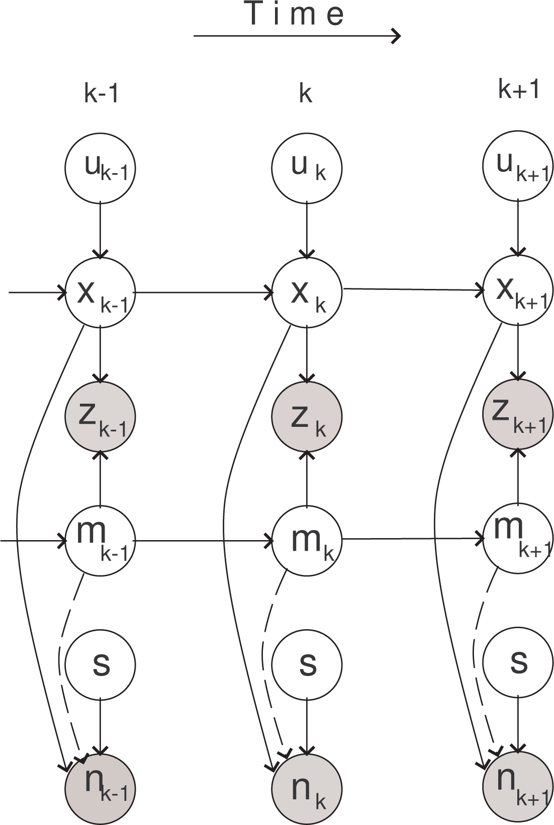
Recursion in Equation (9) involves intractable integrals in the denominator. In order to solve it, we adopt a numerical approximation based on the sequential Monte Carlo method [27]. Before going into details, notice that factorization expressed by Equations (10) and (11) imposes a structure, which can be conveniently represented by a dynamic Bayesian network (DBN) [28] shown in Figure 5. The circles in Figure 5 represent random variables: white circles are hidden variables; gray circles are observed variables. Arrows indicate dependencies. Arrows that are plotted by dashed lines are explained next.

The particle count measurement, n_k, depends on the map, m_k; hence, its likelihood is formulated as g₁(n_k|p_k, m_k, s). The searcher, however, does not know the map (it estimates it only partially as it travels through the search area), and hence, we have introduced the approximate measurement model expressed by Equations (4)–(6). The searcher will therefore process count observations, n_k, using the likelihood function, which is independent of m_k and denoted byg̃₁(n_k|p_k, s), rather than g₁(n_k|p_k, m_k, s). We indicate this fact by drawing the arrow from m_k to n_k in Figure 5 by a dashed line.

The computation of the posterior pdf for a structured complex system, such as the one shown in Figure 5, can be factorised and consequently made computationally and statistically more efficient. Technical details will be given in Section 4.

3.2. Information Driven Motion Control

After processing the measurements received at time k − 1, the searcher needs to select the next control vector, u_k, which will change its position to p_k ∼ p(p_k|p_k−1, u_k). The problem of selecting u_k can be formulated as a partially-observed Markov decision process [29], whose elements are: (1) the set of admissible control vectors $𝒰$_k; (2) the current information state, expressed by the predicted pdf p(y_k|ζ_1:k−1, u_1:k−1, u_k), where u_k ∈ $𝒰$_k; and (3) the reward function associated with each control u_k ∈ $𝒰$_k. In the paper, we adopt motion control based on a single step ahead strategy; this myopic approach is suboptimal in the presence of randomly missing links, but is computationally easier to implement and faster to run. The control vector is then selected as

$${\mathbf{u}}_k=\text{arg}\hspace{0.17em}\underset{\mathbf{v}\in {𝒰}_k}{\text{max}}𝔼\{𝒟(\mathbf{v},p({\mathbf{y}}_k|{\varsigma }_{1:k-1},{\mathbf{u}}_{1:k-1},\mathbf{v}),{\varsigma }_k(\mathbf{v}))\}$$

(12)

where $𝒟$(u, p, ζ) is the reward function. Note that the reward depends on future measurement ${\zeta }_k={\left[n_k{\mathbf{z}}_k^{\text{T}}\right]}^{\text{T}}$, which would be acquired after control u ∈ $𝒰$_k had been applied. Since the decision has to be made before the actual control is applied, the expectation, 𝔼, is taken in Equation (12) with respect to the prior measurements pdf.

Considering that the primary mission of the search is source localisation (map estimation is of secondary importance), the reward function at time k is adopted as the information gain between: (1) the predicted pdf over the state subspace (s, p_k) and (2) the updated pdf over (s, p_k), using the count measurement n_k. The two distributions are denoted π₀(s, p_k|u_k) = p(s|n_1:k−1, u_1:k)p(p_k|p_k−1, u_k) and π₁(s, p_k|n_k, u_k) = ξg̃₁(n_k|p_k, s) π₀(s, p_k|u_k), respectively, where ξ is a normalisation constant. The information gain between the two distributions is measured using a special case of Rényi divergence, known as the Bhattacharyya distance [30]:

$$𝒟({\mathbf{u}}_k)=-2\hspace{0.17em}\text{log}\int \sqrt{{\pi }_1(\mathbf{s},{\mathbf{p}}_k|n_k,{\mathbf{u}}_k)\cdot {\pi }_0(\mathbf{s},{\mathbf{p}}_k|{\mathbf{u}}_k)}d\text{s}\hspace{0.17em}d{\mathbf{p}}_k$$

(13)

where we dropped unnecessary arguments in notation for $𝒟$.

4. The Search Algorithm

The proposed search algorithm, formulated as a DBN with observer control, can be implemented efficiently as a Rao-Blackwellised particle filter (RBPF) [31] with sensor control. Rao-Blackwellisation is a technique for analytical marginalisation of a part of the state vector. Its purpose is to reduce the dimension of the state space in which a Monte Carlo estimation needs to be carried out, in order to improve the computational and statistical efficiency of the particle filter [31,34].

The idea of the RBPF is as follows. Suppose it is possible to divide the components of the hidden state vector, y_k, into two groups, α_k and β_k, such that the following two conditions are satisfied:

• C-1: p(y_k|y_k−1, u_k) = p(α_k|β_k−1:k, α_k−1) · p(β_k|β_k−1, u_k)

• C-2: the conditional posterior distribution p(α_k|β_0:k, ζ_1:k, u_1:k) is analytically tractable.

Then, we need only to estimate the posterior p(β_0:k|ζ_1:k, u_1:k), meaning that we reduced the dimension of the space for Monte Carlo estimation from dim(y_k) to dim(β_k). In the described DBN, shown in Figure 5, in order to satisfy conditions C-1 and C-2, the state vector, y_k, can be partitioned as follows:

$${\alpha }_k={\left[{\mathbf{m}}_k^{\text{T}}\hspace{0.17em}\hspace{0.17em}A\right]}^{\text{T}}$$

(14)

$${\beta }_k={\left[{\mathbf{p}}_k^{⊺}\hspace{0.17em} X\hspace{0.17em} Y\right]}^{⊺}$$

(15)

We are interested only in the filtering posterior density, which can now be factorised as follows:

$$p({\alpha }_k,{\beta }_{0:k}|{\varsigma }_{1:k},{\mathbf{u}}_{1:k})=p({\alpha }_k,|{\beta }_{0:k},{\varsigma }_{1:k},{\mathbf{u}}_{1:k})\cdot p({\beta }_{0:k}|{\varsigma }_{1:k},{\mathbf{u}}_{1:k})$$

(16)

The pdf p(β_0:k|ζ_1:k, u_1:k) is approximated by a random sample ${\left\{{\beta }_{0:k}^{(i)}\right\}}_{i=1}^N$. Subsequently, one can compute analytically (for each sample ${\beta }_{0:k}^{(i)}$):

$$p({\alpha }_k|{\beta }_{0:k}^{(i)},n_{1:k},{\mathbf{z}}_{1:k},{\mathbf{u}}_{1:k})=p({\mathbf{m}}_k,|{\mathbf{z}}_{1:k},{\beta }_{0:k}^{(i)})\cdot p(A|n_{1:k},{\beta }_{0:k}^{(i)})$$

(17)

where:

• $p(m_k|{\mathbf{z}}_{1:k},{\beta }_{0:k}^{(i)})={\mathbf{q}}_k$ is a vector of probabilities of existence for each link in the random grid and

• $p(A|n_{1:k},{\beta }_{0:k}^{(i)})$ is approximated by a Gamma distribution with shape parameter η_k and scale parameter θ_k, i.e., $𝒢$ (A; η_k, θ_k).

Hence, each particle corresponds to a set:

$$\left({\beta }_{0:k}^{(i)},{\mathbf{q}}_k,{\eta }_k,{\theta }_k\right)$$

(18)

where q_k, η_k, θ_k are the sufficient statistics of $p({\alpha }_k|{\beta }_{0:k}^{(i)},n_{1:k},{\mathbf{z}}_{1:k},{\mathbf{u}}_{1:k})$. Keep in mind that q_k, η_k, θ_k depend on a particular sequence (particle) ${\beta }_{0:k}^{(i)}$.

4.1. Recursive Formulae for Sufficient Statistics

Let us first discuss the analytic recursive formula for the computation of q_k, following the ideas of the grid-based SLAM [19]. Note that

$${\mathbf{q}}_k=p({\mathbf{m}}_k{|{\mathbf{z}}_{1:k},\beta }_{0:k}^{(i)})=\frac{g_2({\mathbf{z}}_k{|{\mathbf{m}}_k,\beta }_k^{(i)})p({\mathbf{m}}_k{|{\mathbf{z}}_{k-1},\beta }_{0:k-1}^{(i)})}{{\sum }_{{\mathbf{m}}_k}{g}_2({\mathbf{z}}_k{|{\mathbf{m}}_k,\beta }_k^{(i)})p({\mathbf{m}}_k{|{\mathbf{z}}_{k-1},\beta }_{0:k-1}^{(i)})}$$

(19)

where

$$p({\mathbf{m}}_k|{\mathbf{z}}_{1:k-1},{\beta }_{0:k-1}^{(i)})=\sum _{{\mathbf{m}}_{k-1}}p({\mathbf{m}}_k|{\mathbf{m}}_{k-1})p({\mathbf{m}}_{k-1}|{\mathbf{z}}_{1:k-1},{\beta }_{0:k-1}^{(i)})$$

(20)

The update of probability vector, q_k, is then carried out as follows. Recall from Equation (15) that particle ${\beta }_k^{(i)}$ specifies the location of the searcher at time k, ${\mathbf{p}}_k^{(i)}={\left[x_k^{(i)}\hspace{0.17em}{y}_k^{(i)}\right]}^{⊺}$. Each component of vector z_k is then an observation of existence of a primary or a secondary link from location ${\mathbf{p}}_k^{(i)}$. Let q_j,k−1 be a component of vector q_k−1, denoting the posterior probability that link ℓ_j exists at time k − 1, i.e., $q_{j,k-1}=p(m_{j,k-1}{|\mathbf{z}}_{1:k-1,}{\beta }_{0:k-1}^{(i)})$. Recall also that since the presence or absence of links are assumed independent, then ${\mathbf{q}}_{k-1}={\prod }_{j=1}^L{q}_{j,k-1}$. According to Equation (20), link j existence probability is predicted as

$$q_{j,k|k-1}=p(m_{j,k}=1|m_{j,k-1}=0)\cdot (1-q_{j,k-1})+p(m_{j,k}=1|m_{j,k-1}=1)\cdot q_{j,k-1}.$$

(21)

Let z be a component of vector z_k, which refers to link ℓ_j, according to the current position of the searcher, ${\mathbf{p}}_k^{(i)}$. Then, based on Equation (19), we update the link, j, existence probability as

$$q_{j,k}=\{\begin{array}{cc}\frac{p_d{q}_{j,k|k-1}}{p_d{q}_{j,k|k-1}+p_{fa}(1-q_{j,k|k-1})}& \text{if}\hspace{0.17em} z=1\hspace{0.17em}\\ \frac{(1-p_d)q_{j,k|k-1}}{(1-p_d)q_{j,k|k-1}+(1-p_{fa})(1-q_{j,k|k-1})}& \text{if}\hspace{0.17em} z=0\end{array}$$

(22)

where p_d and p_fa, introduced in Equation (8), are the elements of the appropriate detection Π matrix (primary or secondary) of Equation (8). Equations (19)–(22) can be summarised as:

$${\mathbf{q}}_k=\psi ({\mathbf{q}}_{k-1},{\beta }_k^{(i)},{\mathbf{z}}_k)$$

(23)

Let us describe next the analytic recursion for the update of the parameters, η_k and θ_k, of Equation (18). At time k − 1, the posterior of emission rate A is modeled by a gamma distribution:

$$A|n_{1:k-1},{\beta }_{0:k-1}^{(i)}~𝒢(A;{\eta }_{k-1}{\theta }_{k-1}).$$

(24)

Sensor 1 provides at time k a count measurement, n_k, which plays the key role in the update of parameters η_k−1 and θ_k−1. Recall that the likelihood function of this measurement, ${\tilde{g}}_1(n_k|{\beta }_k^{(i)},A)$, is a Poisson distribution with parameter (mean) ${\lambda }_{k-1}^{(i)}$, rather than A. Fortunately, ${\lambda }_{k-1}^{(i)}$ is linearly related to emission rate A, that is

$${\lambda }_k^{(i)}=A\cdot c({\beta }_k^{(i)})$$

where the constant $c({\beta }_k^{(i)})$ is always positive and given by

$$c_k^{(i)}=-\frac{1}{2}\left(2\hspace{0.17em}\text{log}\hspace{0.17em}{R}_0+\text{log}\frac{{(x_k^{(i)}-X^{(i)})}^2+{(y_k^{(i)}-Y^{(i)})}^2}{{(x_k^{(i)}{Y}^{(i)}-y_k^{(i)}{X}^{(i)})}^2+{(R_0^2-x_k^{(i)}{X}^{(i)}-y_k^{(i)}{Y}^{(i)})}^2}\right)$$

(25)

with X⁽ⁱ⁾ and Y⁽ⁱ⁾, according to Equation (15), being the components of particle ${\beta }_k^{(i)}$.

In the proposed algorithm for the update of parameters η_k−1 and θ_k−1, we use the following two properties of Gamma distribution.

(1)

Scaling property [32]: if X ∼ $𝒢$ (η, θ), then for any c > 0, cX ∼ $𝒢$ (η, cθ).

(2)

Gamma distribution is the conjugate prior of Poisson distributions [33]: if λ ∼ $𝒢$ (η, θ) is a prior distribution and n is a sample from the Poisson distribution with parameter λ, then the posterior is,

$$\lambda ~𝒢(\eta +n,\theta /(1+\theta )).$$

Given ${\beta }_k^{(i)}$, we can compute constant $c_k^{(i)}$ of Equation (25) and express the prior distribution of ${\lambda }_{k-1}^{(i)}$ as

$${\lambda }_{k-1}^{(i)}|n_{1:k-1},{\beta }_{0:k}^{(i)}~𝒢\left(\lambda ;{\eta }_{k-1},c_k^{(i)}\cdot {\theta }_{k-1}\right)$$

(26)

Using measurement n_k and the conjugate prior property, the posterior distribution is

$${\lambda }_{k-1}^{(i)}|n_{1:k-1},{\beta }_{0:k}^{(i)}~𝒢\hspace{0.17em}\left(\lambda ;{\eta }_{k-1}+n_{k,}\frac{c_k^{(i)}\cdot {\theta }_{k-1}}{1+c_k^{(i)}{\theta }_{k-1}}\right)$$

(27)

Since we are after the updated parameters of Gamma distribution of A (rather than ${\lambda }_k^{(i)}$), again, using the scaling property, we have

$$A|n_{1:k},{\beta }_{0:k}^{(i)}~𝒢\hspace{0.17em}\left(A;{\eta }_{k-1}+n_{k,}\frac{{\theta }_{k-1}}{1+c_k^{(i)}{\theta }_{k-1}}\right)$$

(28)

From Equations (24) and (28), we can summarise the analytic expressions for the update of η_k and θ_k as follows

$${\eta }_k={\eta }_{k-1}+{\eta }_k$$

(29)

$${\theta }_k=\frac{{\theta }_{k-1}}{1+c_k^{(i)}{\theta }_{k-1}}.$$

(30)

4.2. Importance Weights

Recursive estimation of p (β_0:k|ζ_1:k, u_1:k) is implemented using a particle filter. If we use the transitional prior as the proposal distribution, i.e.,

$$q({\beta }_{0:k}|{\varsigma }_{1:k},{\mathbf{u}}_{1:k-1})=p({\beta }_k|{\beta }_{k-1},{\mathbf{u}}_k)p({\beta }_{0:k-1}|{\varsigma }_{1:k-1},{\mathbf{u}}_{1:k-1})$$

(31)

the importance weights can be computed recursively as follows [31]:

$$w_k\propto p({\varsigma }_k|{\varsigma }_{1:k-1},{\beta }_{0:k})$$

(32)

For our problem, Expression (32) can be evaluated as

$$\begin{array}{l}{w}_k\propto \int p({\varsigma }_k,{\alpha }_k|{\varsigma }_{1:k-1},{\beta }_{0:k})d{\alpha }_k\\ \hspace{0.17em}\hspace{0.17em}\hspace{0.17em}\hspace{0.17em}\hspace{0.17em}\hspace{0.17em}\hspace{0.17em}=\int {\tilde{g}}_1(n_k|A,{\beta }_k)p(A|n_{1:k-1},{\beta }_{0:k-1})dA\times \end{array}$$

(33)

$$\sum _{{\mathbf{m}}_k}{g}_2({\mathbf{z}}_k|{\mathbf{m}}_k,{\mathbf{p}}_k)p({\mathbf{m}}_k|{\mathbf{z}}_{1:k-1},{\beta }_{0:k-1})$$

(34)

where p(A|n_1:k−1, β_0:k−1) is given by Equation (24) and p(m_k|z_1:k−1, β_0:k−1) = q_k|k−1 by Equation (20), i.e.,

$${\mathbf{q}}_{k|k-1}=\sum _{{\mathbf{m}}_{k-1}}p({\mathbf{m}}_k|{\mathbf{m}}_{k-1}){\mathbf{q}}_{k-1}.$$

The components of vector q_k|k−1, i.e., q_j,k|k−1, were specified by Equation (21). The integral that features in Equation (34) can also be computed analytically. This integral equals

$$ℐ=\int {\tilde{g}}_1(n_k|A,{\beta }_k)p(A|n_{1:k-1},{\beta }_{0:k-1})dA$$

(35)

$$=\int 𝒫(n_k;{\lambda }_k=c({\beta }_k)\cdot A)𝒢(A;{\eta }_{k-1},{\theta }_{k-1})dA$$

(36)

where $𝒫$(n; λ) is the Poisson distribution introduced in Equation (4). Recall the explanation presented in Section 4.1 about the update of the parameters of the Gamma distribution, summarised by Equations (26)–(28). Effectively, we have shown there that

$$𝒢\left(A;{\eta }_{k-1}+n_k,\frac{{\theta }_{k-1}}{1+c_k^{(i)}{\theta }_{k-1}}\right)=\frac{𝒫(n_k;{\lambda }_k=c({\beta }_k)\cdot A)𝒢(A;{\eta }_{k-1},{\theta }_{k-1})}{\int 𝒫(n_k;{\lambda }_k=c({\beta }_k)\cdot A)𝒢(A;{\eta }_{k-1},{\theta }_{k-1})dA}$$

(37)

where the integral in the denominator is $ℐ$; see Equation (36). Hence, the integral can be expressed as

$$ℐ=\frac{𝒫(n_k|{\lambda }_k=c({\beta }_k)\cdot A)𝒢(A;{\eta }_{k-1},{\theta }_{k-1})}{𝒢(A;{\eta }_{k-1}+n_k,{\theta }_{k-1}/(1+c({\beta }_k){\theta }_{k-1}))}$$

(38)

and is computed for an arbitrary chosen value of A > 0. Based on Equation (34), let us summarise the expression for an unnormalised importance weight as

$${\tilde{w}}_k=\phi ({\beta }_k,{\mathbf{q}}_{k-1},{\eta }_{k-1},{\theta }_{k-1},n_k,{\mathbf{z}}_k)$$

(39)

Importance weights determine in a probabilistic manner which particles will survive (and possibly multiply) during the resampling step of the RBPF.

4.3. Information Gain

Suppose the posterior distribution at time k − 1, p(y_k−1|ζ_1:k−1, u_1:k−1), is approximated by a set of particles

$${𝒴}_{k-1}={\left\{\left({\beta }_{k-1}^{(i)},{\mathbf{q}}_{k-1}^{(i)},{\eta }_{k-1}^{(i)},{\theta }_{k-1}^{(i)}\right)\right\}}_{i=1}^N$$

(40)

where random sample ${\beta }_{k-1}^{(i)}$ consists of the searcher position ${\mathbf{p}}_{k-1}^{(i)}={\left[x_{k-1}^{(i)}\hspace{0.17em} y_{k-1}^{(i)}\right]}^{⊺}$ and the position of the source ${\mathbf{p}}_s^{(i)}={\left[X^{(i)}\hspace{0.17em} Y^{(i)}\right]}^{⊺}$; see Equation (15). The weights of the particles in $𝒴$_k−1 are equal, because sensor control is carried out after resampling, i.e., $w_{k-1}^{(i)}=1/N$, i = 1, . . . , N.

The question is how to compute the information gain Equation (13) for each u ∈ $𝒰$_k, based on particles $𝒴$_k−1. We adopt the ideal measurement approximation for this, that is, in hypothesizing the future count measurement (resulting from action u), we assume: (1) action u will be carried out correctly, that is, the transitional density p(p_k|p_k−1, u_k) will be replaced by deterministic mapping; p_k = p_k−1 + u_k; and (2) the measurement count will be equal to the mean of g̃₁(n_k|A, β_k), that is, λ_k (rounded off to the nearest integer).

Since we are after the expected value of the gain, that is, 𝔼{$𝒟$(u)}, we will create an ensemble of “future ideal measurements” ${\left\{n_k^{(j)}\right\}}_{j=1}^M$. Expectation is then approximated by a sample mean, i.e.,

$$𝔼\left\{𝒟(\mathbf{u})\right\}\approx \frac{1}{M}\sum _{j=1}^M{𝒟}^{(j)}(\mathbf{u})$$

where $𝒟$^(j)(u) was computed using $n_k^{(j)}$.

The ensemble of “future ideal measurements” ${\left\{n_k^{(j)}\right\}}_{j=1}^M$ is created as follows. For each action u, choose, at random, a set of M particle indices i_j ∈ {1, . . . , N}, j = 1, . . . , M. Action u is then expected to move the searcher to location ${\mathbf{p}}_k^{(i_j)}={\mathbf{p}}_{k-1}^{(i_j)}+\mathbf{u}$. Then a “future ideal measurement” is $n_k^{(j)}=\lfloor A^{(i_j)}\cdot c^{(i_j)}\rfloor$, where c(^i_j) as a function of ${\mathbf{p}}_k^{(i_j)}$, ${\mathbf{p}}_x^{(i_j)}$ was defined by Equation (25)A(^ij) ∼$𝒢$(A; η_k−1, θ_k−1) and ⌊·⌉ denotes the nearest integer function.

It remains to explain how to compute the gain D^(j)(u) based on $n_k^{(i)}$. Distribution π₀(s, p_k|u_k), which features in Equation (13), can be approximated using the particle set $𝒴$_k−1 as follows:

$${\pi }_o(\mathbf{s},{\mathbf{p}}_k\mathbf{u})\approx 𝒢(A;{\eta }_{k-1}{\theta }_{k-1})\sum _{i=1}^N{w}_{k-1}^{(i)}\delta ({\mathbf{p}}_s-{\mathbf{p}}_s^{(i)},{\mathbf{p}}_k-{\mathbf{p}}_k^{(i)})$$

(41)

where ${\mathbf{p}}_k^{(i)}~p({\mathbf{p}}_k|{\mathbf{p}}_{k-1}^{(i)},\mathbf{u})$. The updated distribution is

$${\pi }_1(\mathbf{s},{\mathbf{p}}_k|\mathbf{u},n_k^{(i)})=\frac{{\tilde{g}}_1(n_k^{(i)}|{\mathbf{p}}_k,{\mathbf{p}}_s,A){\pi }_o(\mathbf{s},{\mathbf{p}}_k|\mathbf{u})}{\int {\tilde{g}}_1(n_k^{(i)}|{\mathbf{p}}_k,{\mathbf{p}}_s,A){\pi }_o(\mathbf{s},{\mathbf{p}}_k|\mathbf{u})d\mathbf{s}d{\mathbf{p}}_k}.$$

(42)

Substitution of Equations (41) and (42) into Equation (13) leads to

$${𝒟}^{(i)}(\mathbf{u})\approx -2\hspace{0.17em}\text{log}\frac{{{\sum }_{i=1}^N{w}_{k-1}^{(i)}𝒥}^{(i)}(n_k^{(i)})}{{\left[{\sum }_{i=1}^N{w}_{k-1}^{(i)}{ℐ}^{(i)}(n_k^{(i)})\right]}^{1/\mathrm{2\hspace{0.17em}}}}$$

(43)

where $ℐ$⁽ⁱ⁾(n_k) is computed via Equation (38) and

$${𝒥}^{(i)}(n_k)=\int {\left[𝒫(n_k;{\lambda }_k^{(i)}=c({\beta }_k^{(i)})A)\right]}^{1/2}\times 𝒢(A;{\eta }_{k-1}^{(i)},{\theta }_{k-1}^{(i)})dA.$$

(44)

The integral in Equation (44) can be evaluated numerically.

4.4. Implementation

The pseudo-code of one cycle of the search algorithm is presented in Algorithm 1. The input consists of the particle set, $𝒴$_k−1, defined by Equation (40). Selection of the control vector, u_k (line 2 of Algorithm 1), is described in Algorithm 2.

An explanation of the steps in Algorithm 1 is described first. Estimation of the state vector via the RBPF is carried out in lines 4–18. According to Equation (15), random vector ${\beta }_{k-1}^{(i)}$ consists of ${\mathbf{p}}_{k-1}^{(i)}$, X⁽ⁱ⁾ and Y⁽ⁱ⁾. Since the source location, (X⁽ⁱ⁾, Y⁽ⁱ⁾), is static, only the component, ${\mathbf{p}}_{k-1}^{(i)}$, is propagated to future time k in line 6. In line 7, Equation (39) is applied to compute the unnormalised weights of each particle. The map, represented by the probability of existence of each link, is updated in line 8, based on the Expression (23). The parameters of Gamma distribution are update in lines 9–11. The weights assigned to each quadruple ( ${\beta }_k^{(i)}$, ${\mathbf{q}}_k^{(i)}$, ${\eta }_k^{(i)}$, ${\theta }_k^{(i)}$) are normalised in line 14. Resampling of particles is carried out in lines 15p–18. The particles for source position ${\mathbf{p}}_s^{(i)}$ are not restricted to the grid nodes and after the resampling step, their diversity is improved by regularisation [34]. Finally, the output is the particle set, $𝒴$_k.

Algorithm 1:. The searcher algorithm.

1:	Input: $𝒴$k−1
2:	Run Algorithm 2 to select the control vector uk
3:	Apply control uk and collect measurements zk, nk
4:	Ȳ;k = ∅; $𝒴$k = ∅
5:	for i =1, . . . ,N do
6:	Draw ${\mathbf{p}}_k^{(i)}~p({\mathbf{p}}_k|{\mathbf{p}}_{k-1}^{(i)},{\mathbf{u}}_k)$
7:	${\tilde{w}}_k^{(i)}=\phi ({\beta }_k^{(i)},{\mathbf{q}}_{k-1}^{(i)},{\eta }_{k-1}^{(i)},{\theta }_{k-1}^{(i)},n_k,z_k)$
8:	${\mathbf{q}}_k^{(i)}=\psi ({\mathbf{q}}_{k-1}^{(i)},{\beta }_k^{(i)},{\mathbf{z}}_k)$
9:	${\eta }_k^{(i)}={\eta }_{k-1}^{(i)}+n_k$
10:	Compute constant $C_k^{(i)}$ as a function of ${\beta }_k^{(i)}$ using Equation (25)
11:	${\theta }_k^{(i)}={\theta }_{k-1}^{(i)}/(1+c_k^{(i)}{\theta }_{k-1}^{(i)})$
12:	${\overline{𝒴}}_k={\overline{𝒴}}_k\cup \left\{({\beta }_k^{(i)},{\mathbf{q}}_k^{(i)},{\eta }_k^{(i)},{\theta }_k^{(i)})\right\}$
13:	end for
14:	$w_k^{(i)}={\tilde{w}}_k^{(i)}/{\sum }_{j=1}^N{\tilde{w}}_k^{(i)},\text{for}\hspace{0.17em}i=1,\dots ,N$
15:	for i = 1, . . . ,N do
16:	Select index ji ∈ {1, . . . ,N} with probability $w_k^{(i)}$
17:	${\overline{𝒴}}_k={\overline{𝒴}}_k\cup \left\{({\beta }_k^{(i)},{\mathbf{q}}_k^{(i)},{\eta }_k^{(j_i)},{\theta }_k^{(j_i)})\right\}$
18:	end for
19:	Output: $𝒴$k

Algorithm 1:. The searcher algorithm.

1:	Input: $𝒴$k−1
2:	Run Algorithm 2 to select the control vector uk
3:	Apply control uk and collect measurements zk, nk
4:	Ȳ;k = ∅; $𝒴$k = ∅
5:	for i =1, . . . ,N do
6:	Draw ${\mathbf{p}}_k^{(i)}~p({\mathbf{p}}_k|{\mathbf{p}}_{k-1}^{(i)},{\mathbf{u}}_k)$
7:	${\tilde{w}}_k^{(i)}=\phi ({\beta }_k^{(i)},{\mathbf{q}}_{k-1}^{(i)},{\eta }_{k-1}^{(i)},{\theta }_{k-1}^{(i)},n_k,z_k)$
8:	${\mathbf{q}}_k^{(i)}=\psi ({\mathbf{q}}_{k-1}^{(i)},{\beta }_k^{(i)},{\mathbf{z}}_k)$
9:	${\eta }_k^{(i)}={\eta }_{k-1}^{(i)}+n_k$
10:	Compute constant $C_k^{(i)}$ as a function of ${\beta }_k^{(i)}$ using Equation (25)
11:	${\theta }_k^{(i)}={\theta }_{k-1}^{(i)}/(1+c_k^{(i)}{\theta }_{k-1}^{(i)})$
12:	${\overline{𝒴}}_k={\overline{𝒴}}_k\cup \left\{({\beta }_k^{(i)},{\mathbf{q}}_k^{(i)},{\eta }_k^{(i)},{\theta }_k^{(i)})\right\}$
13:	end for
14:	$w_k^{(i)}={\tilde{w}}_k^{(i)}/{\sum }_{j=1}^N{\tilde{w}}_k^{(i)},\text{for}\hspace{0.17em}i=1,\dots ,N$
15:	for i = 1, . . . ,N do
16:	Select index ji ∈ {1, . . . ,N} with probability $w_k^{(i)}$
17:	${\overline{𝒴}}_k={\overline{𝒴}}_k\cup \left\{({\beta }_k^{(i)},{\mathbf{q}}_k^{(i)},{\eta }_k^{(j_i)},{\theta }_k^{(j_i)})\right\}$
18:	end for
19:	Output: $𝒴$k

The selection of a control vector, described by Algorithm 2, starts with postulating the set, $𝒰$_k, in line 2. For every u ∈ $𝒰$_k, the algorithm anticipates j = 1, . . . , M future measurements $n_k^{(j)}$ (line 9) and accordingly computes a sample of the reward $𝒟$^(j)(u) (line 14). The expected reward is then a sample mean (line 16). Finally, the optimal one-step ahead control is selected in line 18.

It has been observed in simulations that one step ahead control can sometimes lead to situations where the observer position switches eternally between two or three nodes of the lattice. In order to overcome this problem, we adopt a heuristic as follows: if a node has been visited in the last 10 search steps more than three times, the next motion control vector is selected at random. While a multi-step ahead searcher control would be preferable than the adopted heuristic, it would also be computationally more demanding. Multi-step ahead searcher control remains to be explored in future work.

Algorithm 2:. Selection of control vector.

1:	Input: $𝒴$k−1
2:	Create the set of admissible controls $𝒰$k = {·,→,←,↑,↓}
3:	for every u ∈ $𝒰$k do
4:	for j = 1, . . . ,M do
5:	Choose at random particle index ij ∈ {1, . . . ,N}
6:	${\mathbf{p}}_k^{(i_j)}={\mathbf{p}}_{k-1}^{(i_j)}+\mathbf{u};$
7:	Compute $c_k^{(i_j)}$ using ${\mathbf{p}}_k^{(i_j)}$ and ${\mathbf{p}}_s^{(i_j)}$ via Equation (25)
8:	Adopt $A^{(i_j)}={\eta }_{k-1}^{(i_j)}\cdot {\theta }_{k-1}^{(i_j)}$
9:	${\eta }_k^{(j)}=\lfloor A_{k-1}^{(i_j)}\cdot {\theta }_{k-1}^{(i_j)}\rfloor$
10:	for i = 1, . . . ,N do
11:	Compute ${ℐ}^{(i)}(n_k^{(j)})$ via Equation (38)
12:	Compute ${𝒥}^{(i)}(n_k^{(j)})$ via Equation (44)
13:	end for
14:	Compute $𝒟$(j)(u) using Equation (43)
15:	end for
16:	Estimate 𝔼{$𝒟$(u)} as a sample mean of ${\left\{{𝒟}^{(j)}(\mathbf{u})\right\}}_{j=1}^M$
17:	end for
18:	Select control vector uk ∈ $𝒰$k using Equation (12)

Algorithm 2:. Selection of control vector.

1:	Input: $𝒴$k−1
2:	Create the set of admissible controls $𝒰$k = {·,→,←,↑,↓}
3:	for every u ∈ $𝒰$k do
4:	for j = 1, . . . ,M do
5:	Choose at random particle index ij ∈ {1, . . . ,N}
6:	${\mathbf{p}}_k^{(i_j)}={\mathbf{p}}_{k-1}^{(i_j)}+\mathbf{u};$
7:	Compute $c_k^{(i_j)}$ using ${\mathbf{p}}_k^{(i_j)}$ and ${\mathbf{p}}_s^{(i_j)}$ via Equation (25)
8:	Adopt $A^{(i_j)}={\eta }_{k-1}^{(i_j)}\cdot {\theta }_{k-1}^{(i_j)}$
9:	${\eta }_k^{(j)}=\lfloor A_{k-1}^{(i_j)}\cdot {\theta }_{k-1}^{(i_j)}\rfloor$
10:	for i = 1, . . . ,N do
11:	Compute ${ℐ}^{(i)}(n_k^{(j)})$ via Equation (38)
12:	Compute ${𝒥}^{(i)}(n_k^{(j)})$ via Equation (44)
13:	end for
14:	Compute $𝒟$(j)(u) using Equation (43)
15:	end for
16:	Estimate 𝔼{$𝒟$(u)} as a sample mean of ${\left\{{𝒟}^{(j)}(\mathbf{u})\right\}}_{j=1}^M$
17:	end for
18:	Select control vector uk ∈ $𝒰$k using Equation (12)

5. Numerical Results

5.1. Illustrative Runs

We applied the described search algorithm to the search area modelled by the random grid shown in Figure 2. Prior knowledge available to the searcher is illustrated by Figure 1: the radius of the search area is R₀ = 9; the centre is c = (0, 0), and the total number of potential links in the complete grid modelling the search area is L = 572. The parameters of the emitting source to be estimated are: X = 0, Y = 7 and A₀ = 12. The searcher initial position is p₀ = (9, −4).

Dynamic model p(m_k|m_k−1) is a 2 × 2 transitional probability matrix with diagonal and off-diagonal elements 0.999 and 0.001, respectively, meaning the changes in the status of the links are very rare. This ensures a stable structure of the search domain, because the count measurement model is valid in a steady state. Dynamic model p(p_k|p_k−1, u_k) can be expressed as

$$p({\mathbf{p}}_k|{\mathbf{p}}_{k-1},{\mathbf{u}}_k)=(1-p_e)\delta ({\mathbf{p}}_k-{\mathbf{p}}_{k-1}+{\mathbf{u}}_k)+\sum _{\text{v}\in {𝒰}_k\backslash {\mathbf{u}}_k}\frac{p_e}{|{𝒰}_k|-1}\delta ({\mathbf{p}}_k-{\mathbf{p}}_{k-1}+\mathbf{v})$$

(45)

where, in simulations, we used the value p_e = 0.04.

The parameters of detection matrices, which define the likelihood function g₂(z_k|p_k, m_k), are as follows: for primary observable links, p_d = 1 and p_fa = 0; for secondary observable links, p_d = 0.8 and p_fa = 0.1.

The RBPF used N = 4, 000 particles with M = 400 samples used in the averaging of information gain. The particle set, $𝒴$₀, at the initial time is created as follows: ${\mathbf{p}}_0^{(i)}={\mathbf{p}}_0$, for all i = 1, . . . , N particles; the source location vector is drawn from a uniform distribution over a circle with centre c and radius R₀, i.e., ${\mathbf{p}}_s^{(i)}~{𝒰}_{\text{Circle}(\text{c},R_0)}({\mathbf{p}}_s)$; link existence probabilities are set to q_j,0 = 0.5, for all j = 1, . . . , L links; finally, the parameters of initial Gamma distribution $𝒢$(A; η₀, θ₀) were selected as η₀ = 15 and θ₀ = 1.

We terminate the search algorithm when the searcher steps on the source. At this point, we compare the true source location with the current estimate of the posterior distribution of the searcher position, approximated by particles ${\left\{{\mathbf{p}}_k^{(i)}\right\}}_{i=1}^N$. If the true source position is contained in the support defined by ${\left\{{\mathbf{p}}_k^{(i)}\right\}}_{i=1}^N$, the search is considered successful.

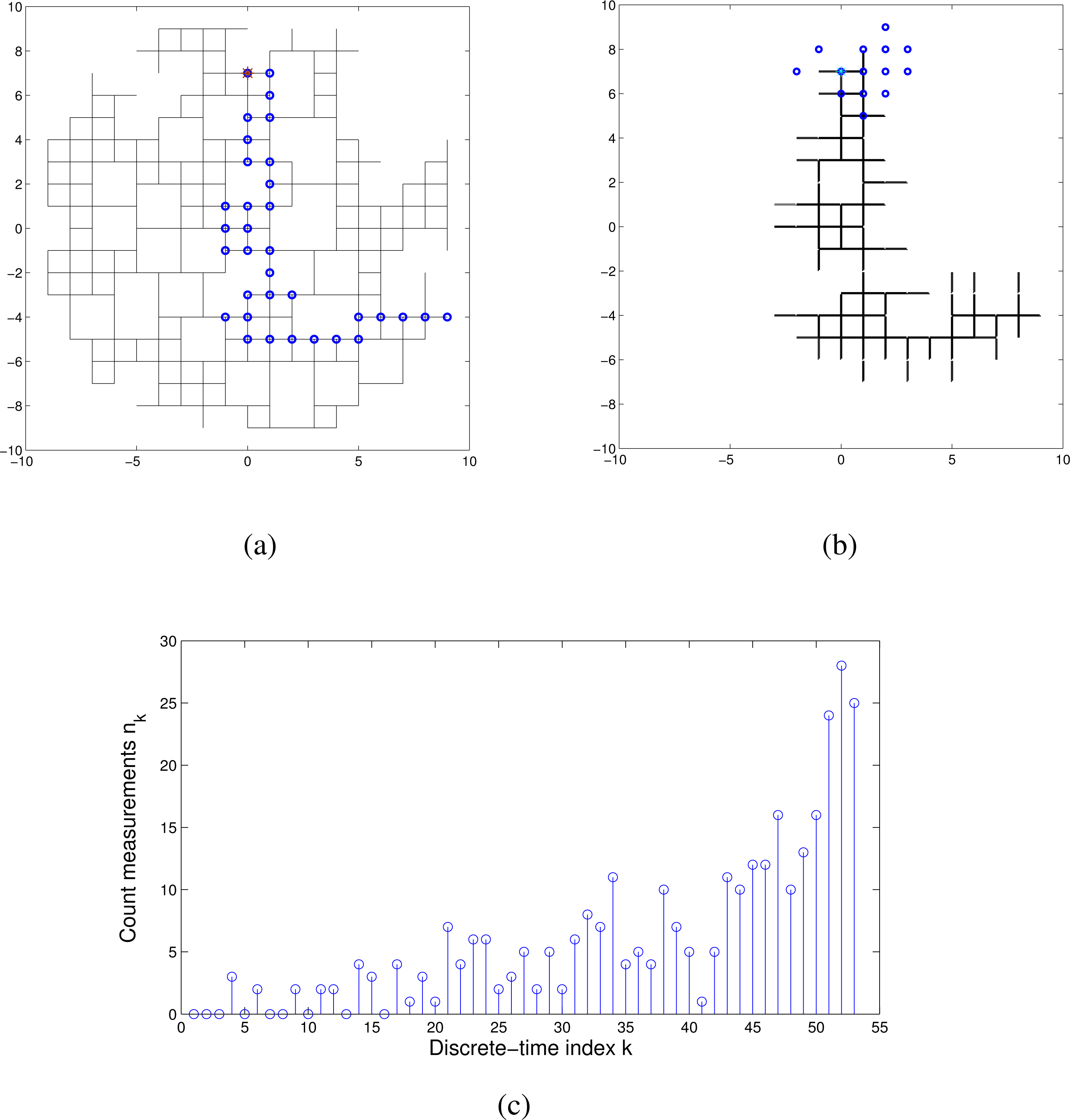
Figure 6 illustrates a typical run of the search algorithm. The true path of the searcher on this run is shown in Figure 6a. It took the searcher 53 time steps to reach the source. During the search, the motion control vector failed to execute correctly on two occasions. The final estimate of the map (i.e., of existing links of the square lattice) is shown in Figure 6b. This figure shows only the links whose probability of existence is higher than 0.6. The blue circles in Figure 6b indicate the posterior distribution of the searcher final position. Its true position, which is the same as the source position, is included in the support of this posterior, meaning that the search was successful. Moreover, on this occasion, the maximum a posteriori (MAP) estimate of the searcher final position coincides with the truth. Figure 6c shows the measured values of the count number, n_k, along the path. As we discussed in the Introduction, the measurements are sporadic, especially in the beginning, when the distance between the searcher and the source is large: among the first ten count measurements, only three indicated a non-zero tracer concentration. An avi video file, illustrating a single run of the algorithm, is supplied with this paper.

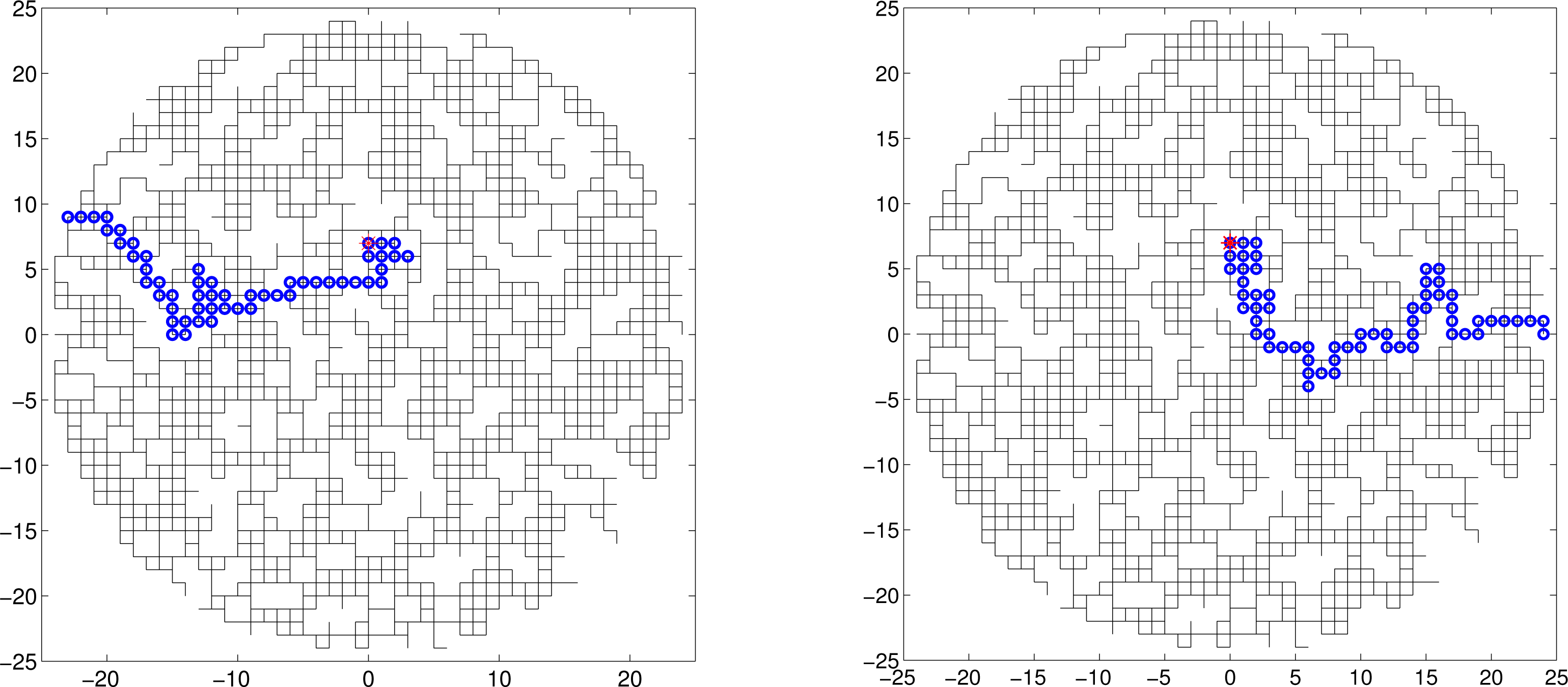
Figure 7 illustrates two search paths on a much bigger lattice, with the fraction of missing links p = 0.20. The source parameters were X = 0, Y = 7 and A₀ = 16; all other parameters were the same as above. The duration of two searches was 84 and 103 time steps, respectively.

5.2. Monte Carlo Runs

The average performance of the search algorithm has been assessed via Monte Carlo runs using the smaller scale model of the search area (and its corresponding parameters), shown in Figure 6. If the search on a particular run was successful, its corresponding search time is used in averaging. A run is declared unsuccessful if the source has not been found after k = 100 discrete-time steps. We also keep the statistics on the success rate of the search. The results obtained via averaging over 100 Monte Carlo runs are presented in

Table 1. The average performance of the search algorithm: different source locations, A₀ = 12.

Source location	Shortest path length	Number of search steps	Success rate
(0, 7)	20	42.1	94
(0, 1)	14	34.0	95
(2, −5)	8	28.8	99

for three different locations of the source, i.e., (X, Y) = (0, 7), (0, 1), (2, −5). The three locations correspond to the shortest path distances (from the searcher initial position p₀ = (9, −4) to the source) of 20, 14 and eight unit lengths, respectively. All other parameters were the same as described above for the illustrative run. As expected, the results in Table 1 indicate that the search is quicker and more reliable (i.e., with a higher success rate) for a source which is closer to the searcher initial position.

Table 2. The average performance of the search algorithm: different source release-rates, source location (0, 7).

Release rate A0	Number of search steps	Success rate [%]
8	49.5	78
12	42.1	94
16	38.2	93

presents the results for a source at location (0, 7), but with three different values of the source release-rate, i.e., A₀ = 8, 12, 16. The results indicate that the search is quicker for a source characterised by a higher release rate. The explanation of this trend is as follows. Initially, when the searcher is far from the source, its measurements of tracer concentration are very small, typically zero, hence uninformative. During this phase of the search, the searcher effectively moves according to a “diffusive” (or random walk) model, which is slower than the so-called “ballistic” movement associated with an information-driven search [2]. The random walk phase is longer for a weaker source, which contributes to the overall longer search time in this case. As a specific numerical example, we have also validated that a purely random search never manages to find the source at (0, 7) in the given time frame of 100 discrete time steps.

6. Summary

The paper considers a very difficult problem of autonomous search for a diffusive point source of tracer in an environment whose structure is unknown. Sequential estimation and motion control are carried out in highly uncertain circumstances with the state space, including, in addition to the source parameters, the map of the search area and the searcher position within the map. The paper develops mathematical models of measurements, formulates the sequential Bayesian solution (in the form of a Rao-Blackwellised particle filter) and proposes an information-driven motion control of the searcher. The numerical results demonstrate the concept, indicating high success rates in comparison with a random walk. A gradient-based search (“chemotaxis”) would be inappropriate in this application, because the computation of a gradient is infeasible in the presence of intermittent measurements and geometric constraints.

There are many areas for further research and improvements of the concepts introduced in this paper. One direction is to explore the potential benefits of the analytical results available from percolation theory in the theoretical analysis of searcher performance. Another is to investigate more efficient particle filters for source parameter estimation (being a deterministic part of the state space) and search strategies that “look” multiple steps ahead (rather than a one step myopic search). It is also desirable to further explore the coordination of multiple networked searchers with decentralised estimation and motion control. Finally, it would be important to practically validate the proposed autonomous searcher in experimental trials.

References

- Viswanathan, G.M.; Afanasyev, V.; Buldyrev, S.V.; Murphy, E.J.; Prince, P.A.; Satnley, H.E. Levy flight search patterns of wandering albatrosses. Nature 1996, 381, 413–415. [Google Scholar]
- Bénichou, O.; Loverdo, C.; Moreau, M.; Voituriez, R. Intermittent search strategies. Rev. Mod. Phys 2011, 83, 81–129. [Google Scholar]
- Hein, A.M.; McKinley, S.A. Sensing and decision-making in random search. Proc. Natl. Acad. Sci. USA 2012, 109. [Google Scholar] [CrossRef]
- Coppey, M.; Benichou, O.; Voituriez, R.; Moreau, M. Kinetics of target site localization of a protein on DNA: A stochastic approach. J. Biophys 2004, 87, 1640–1649. [Google Scholar]
- Bressloff, P.C.; Newby, J. Filling of a Poisson trap by a population of random intermittent searchers. Phys. Rev. E 2012, 85, 031909. [Google Scholar]
- Holcman, D. Modeling DNA and Virus Trafficking in the Cell Cytoplasm. J. Stat. Phys 2007, 127, 471–494. [Google Scholar]
- Bressloff, P.C.; Newby, J. Stochastic models of intracellular transport. J. Chem. Phys 2013, 85, 135–196. [Google Scholar]
- Farrell, J.A.; Pang, S.; Li, W. Plume mapping via Hidden Markov methods. IEEE Trans. Syst. Man Cybern 2003, 33, 850–863. [Google Scholar]
- Li, W.; Farrell, J.A.; Pang, S.; Arrieta, R.M. Moth-inspired chemical plume tracking on an autonomous underwater vehicle. IEEE Trans. Robot 2006, 22, 292–307. [Google Scholar]
- Oyekan, J.; Hu, H. A novel bio-controller for localizing pollution sources in a medium peclet environment. J. Bionic Eng 2010, 7, 345–353. [Google Scholar]
- Klimenko, A.V.; Priedhorsky, W.C.; Hengartner, N.W.; Borozin, K.N. Efficient strategies for low-level nuclear searches. IEEE Trans. Nucl. Sci 2006, 53, 1435–1442. [Google Scholar]
- Ristic, B.; Gunatilaka, A. Information driven localisation of a radiological point source. Inf. Fusion 2008, 9, 317–326. [Google Scholar]
- Ristic, B.; Morelande, M.; Gunatilaka, A. Information driven search for point sources of gamma radiation. Signal Process 2010, 90, 1225–1239. [Google Scholar]
- Ishida, H.; Nakayama, G.; Nakamoto, T.; Morizumi, T. Controlling a Gas/Odor plume tracking robot based on transient responses of gas sensors. IEEE Sens. J 2005, 5, 537–545. [Google Scholar]
- Dhariwal, A.; Sukhatme, G.S.; Requicha, A.A.G. Bacterium-Inspired Robots for Environmental Monitoring. In Proceedings of IEEE International Conference on Robotics and Automation (ICRA’04), New Orleans, LA, USA, 26 April–1 May 2004; pp. 1436–1443.
- Vergassola, M.; Villermaux, E.; Shraiman, B.I. ‘Infotaxis’ as a strategy for searching without gradients. Nature 2007, 445, 406–409. [Google Scholar]
- Iacono, G.L. A comparison of different searching strategies to locate sources of odor in turbulent flows. Adapt. Behav 2010, 18, 155–170. [Google Scholar]
- Masson, J.B. Olfactory searches with limited space perception. Proc. Natl. Acad. Sci. USA 2013, 110. [Google Scholar] [CrossRef]
- Thrun, S.; Burgard, W.; Fox, D. Probabilistic Robotics; MIT Press: Cambridge, MA, USA, 2005. [Google Scholar]
- Ben-Avraham, D.; Havlin, S. Diffusion and Reaction in Fractals and Disordered Systems; Cambridge University Press: Cambridge, UK, 2000. [Google Scholar]
- Torquato, S. Random Heterogeneous Materials: Microstructure and Macroscopic Properties; Springer: New York, NY, USA, 2002. [Google Scholar]
- Kemeny, J.G.; Snell, J.L. Finite Markov Chains; Van Nostrand Reinhold Company: New York, NY, USA, 1960. [Google Scholar]
- Prosperetti, A. Advanced Mathematics for Applications; Cambridge University Press: Cambridge, UK, 2011. [Google Scholar]
- Marjovi, A.; Marques, L. Multi-robot olfactory search in structured environments. Robot. Auton. Syst 2011, 59, 867–881. [Google Scholar]
- Selvadurai, A.P.S. Partial Differential Equations in Mechanics 1; Springer: Berlin, Germany, 2000. [Google Scholar]
- Burioni, R.; Cassi, D. Random walks on graphs: Ideas, techniques and results. J. Phys. A Math. Gen 2005, 38. [Google Scholar] [CrossRef]
- Doucet, A., de Freitas, J.F.G., Gordon, N.J., Eds.; Sequential Monte Carlo Methods in Practice; Springer: New York, NY, USA, 2001.
- Dean, T.; Kanazawa, K. A model for reasoning about persistence and causation. Comput. Intell 1989, 5, 142–150. [Google Scholar]
- Chong, E.; Kreucher, C.; Hero, A. POMDP Approximation Using Simulation and Heuristics. In Foundations and Applications of Sensor Management; Hero, A., Castanon, D., Cochran, D., Kastella, K., Eds.; Springer: New York, NY, USA, 2008; Chapter 8. [Google Scholar]
- Kailath, T. The divergence and Bhattacharyya distance measures in signal selection. IEEE Trans. Commun. Tech 1967, 15, 52–60. [Google Scholar]
- Doucet, A.; de Freitas, N.; Murphy, K.P.; Russell, S.J. Rao-Blackwellised Particle Filtering for Dynamic Bayesian Networks. In Proceedings of the 16th Conference on Uncertainty in Artificial Intelligence, Stanford, CA, USA, 30 June–3 July 2000; pp. 176–183.
- Hazewinkel, M. Gamma-Distribution. Encyclopedia of Mathematics, Available online: http://www.encyclopediaofmath.org/index.php?title=Gamma-distribution&oldid=24074 (accessed on 10 February 2014).
- Gelman, A.; Carlin, J.B.; Stern, H.S.; Dunson, D.B.; Vehtari, A.; Rubin, D.B. Bayesian Data Analysis, 3nd ed; CRC Press: Boca Raton, FL, USA, 2003. [Google Scholar]
- Ristic, B.; Arulampalam, S.; Gordon, N. Beyond the Kalman Filter: Particle Filters for Tracking Applications; Artech House: Boston, MA, USA, 2004. [Google Scholar]
- Nicholson, C. Diffusion and related transport mechanisms in brain tissue. Rep. Prog. Phys 2001, 64, 815–884. [Google Scholar]
- Novak, I.L.; Kraikivski, P.; Slepchenko, B.M. Diffusion in cytoplasm: Effects of excluded volume due to internal membranes and cytoskeletal structures. Biophys. J 2009, 97, 758–767. [Google Scholar]
- Pisani, L. Simple expression for the tortuosity of porous media. Transp. Porous Media 2011, 88, 193–203. [Google Scholar]