Cross Layer Interference Management in Wireless Biomedical Networks

Abstract

Interference, in wireless networks, is a central phenomenon when multiple uncoordinated links share a common communication medium. The study of the interference channel was initiated by Shannon in 1961 and since then this problem has been thoroughly elaborated at the Information theoretic level but its characterization still remains an open issue. When multiple uncoordinated links share a common medium the effect of interference is a crucial limiting factor for network performance. In this work, using cross layer cooperative communication techniques, we study how to compensate interference in the context of wireless biomedical networks, where many links transferring biomedical or other health related data may be formed and suffer from all other interfering transmissions, to allow successful receptions and improve the overall network performance. We define the interference limited communication range to be the critical communication region around a receiver, with a number of surrounding interfering nodes, within which a successful communication link can be formed. Our results indicate that we can achieve more successful transmissions by adapting the transmission rate and power, to the path loss exponent, and the selected mode of the underline communication technique allowing interference mitigation and when possible lower power consumption and increase achievable transmission rates.

1. Introduction

Recent advances in Information and Communications Technology (ICT) enable the acquisition, transmission and interpretation of different bio-signals, from fixed or mobile locations. This can support better prevention and well-being and provide valuable and prompt diagnostic tools in various application domains, ranging from home care to emergency care, or situations in which a second or a specialist opinion is required before making a clinical decision [1]. Important trends in healthcare include citizen mobility and the consequent shift towards shared or integrated care where the single doctor-patient relationship has evolved to one in which each individual’s healthcare is the responsibility of a team of professionals in a geographically extended healthcare system. In such a new setting, the possibility of collecting clinical information from different points is becoming a common need for citizens and physicians. In this perspective, with focus to the provision of high quality of care, assuring life independency, personalized medicine, the significant new research challenge is the integration of multiple biomedical sensor streams, to extract local and global health-state indicator variables that can be queried and monitored in an unobtrusive way [2].

Wireless biomedical networks serve as the transport mechanism among devices or between devices and traditional backbone networks allowing the transmission of health related information [3]. In this type of networking environment wireless sensing and communication technologies are used to allow acquisition of various bio-signals for subsequent monitoring and analysis [4]. Biomedical body/personal wireless sensor networks have been extensively applied in remote health monitoring and patient care [5,6] allowing wireless, wearable or implanted vital sign sensors to be continuously sampled, such as EEG [7], ECG, SpO2, weight, blood pressure, heart rate[8], etc. Although such kinds of networks share many similar properties with general-purpose wireless networks, many domain specific challenges (related to power consumption, transmission range, high degree of reliability, security, etc.) have emerged with respect to specific application domain requirements [9]. A review of applications in healthcare that use wireless biomedical networks and related issues and challenges including interference effect on the network performance is presented in [10]. Today, wireless biomedical communication technologies empower the development of new applications and services to improve the quality of medical care provided to the citizens through ubiquitous healthcare environments [5,6,11,12] raising two crucial issues: (a) RF transmissions can cause electromagnetic interference among biomedical devices, which could as a result critically malfunction or conclude with unsuccessful transmission [13] and (b) different types of electronic health (e-Health) applications and services require different quality of service support [14,15]. It is thus evident that current advances in wireless communication technologies are transforming the delivery of health care. The emphasis is towards personalized and pervasive mobile monitoring focusing on the development of innovative health services to empower individuals in well-being and disease prevention, as well as chronic disease management [16]. These services use a wide range of wireless medical devices and sensors and wireless telecommunication infrastructures to allow ubiquitous remote biomedical monitoring [17–20].

The objective of this work is to present an in-depth analysis of how cross layer techniques can be used in the design and study of wireless biomedical networks. More specifically, we study how, by adapting various parameters of the telecommunication system, we can: (i) allow more concurrent transmissions; (ii) minimize interference; (iii) enhance network throughput; (iv) maximize individual link data rates; and (v) optimally utilize network resources for all competing transmissions. We present our theoretical analysis and simulation results taking into account the number of interfering nodes, and networking parameters of the underline telecommunication system. We investigate how a medium access mechanism, using cross layer cooperative communication techniques [21], can be used for interference compensation at a receiving node from all other interfering transmissions in range and allow successful reception of the signal of interest and thus improve the overall network performance in a seamless and cooperative way to allow different types of health related services and data to be successfully transferred through the wireless medium.

Most state-of-the-art systems deal with interference in one of the following two ways, even though both of them might be sub-optimal, either: (a) orthogonalize the communication links in time or frequency so that they do not interfere with each other at all; or (b) allow communication links to share the same degrees of freedom, but treat each other’s interference as adding to the noise floor. The first approach entails an a priori loss of degrees of freedom in both links, no matter how weak the potential interference is. The second approach treats interference as noise, while it actually carries information and has structure that can potentially be exploited in mitigating its effect. These considerations lead to the natural question of what is the best performance one can achieve without making any a priori assumptions on how the common resource is shared.

A basic information theory model to study this question is the two-user Gaussian interference channel, where two point-to-point links with additive white Gaussian noise interfere with each other. Recent work on the interference channel [22] has shown the frontiers for the achievable rate regions for a n-user interference channel determining the shape and size of the rate regions. The usual assumptions in previous works lies in the fact that interference is considered as additional noise and that the maximum achievable rate depends logarithmically on the Signal to Interference and Noise Ratio (SINR). The exact calculation of the interference in a wireless ad hoc network is a difficult task even when special algorithms are used to share information of power and distances among network nodes.

Many known studies try to model and calculate interference levels for a wireless multi-hop ad hoc network, taking into account the number of nodes, density of nodes, radio propagation, predefined position of interfering nodes and the amount of relay traffic [23–25]. The two-user interference channel stability region has been studied in [26] using stochastic dominance techniques also considering the case that each receiver treats interference as Gaussian noise or by employing successive interference cancelation. The work presented in [27] characterizes the capacity region for the two-user Gaussian interference channel within one bit showing that, treating interference as noise, achieves the sum capacity of the two-user Gaussian interference channel in low-interference. Further studies shows that under specific conditions two strongly interfering communication links with additive white Gaussian noise can achieve rates as high as would be achievable without this interference [28]. In [29] upper and lower capacity order-bounds are derived using the concept of the exclusion region to limit interference caused to the receiver. It is shown that the network capacity decreases when the size of the exclusion region (a region around each receiver such that nodes inside it are not allowed to transmit) increases. In [30], the size of the exclusion region is studied, for which an optimal size that maximizes capacity is suggested and is shown to depend on the density of the network nodes.

Our goal, in this work, is to control the amount of interference experienced by receivers and, in certain cases, to enforce concurrent transmissions, in order to maximize network performance by tightly coupling both physical and medium access layers. We examine a simplified wireless telecommunication system, which is used as the medium to transmit biomedical data, where randomly distributed networking nodes use a specific modulation scheme with a specific Bit-Error-Rate (BER) and a constant bandwidth assuming the absence of any error control coding or any multiuser decoding scheme or any cooperation between transmitters and/or receivers. This model reflects the situation of multiple low power/low complexity communication networks such as sensor networks, suitable to work in a networking biotelemetry system, and it enables us to make observations, with practical significance, for the operation of these networks. We study how interference, separation distance, power and rate adaptation, for biomedical telemetry wireless communications, can allow concurrent transmissions, enhance network capacity by maximizing, when possible, individual link data rates, minimize transfer time of a data packet and allow the best possible usage of network’s resources for all competing transmissions. Higher transmission rates can be achieved with higher levels of modulation (M-ary modulation), but higher transmission power is required to maintain acceptable bit error rate performance. If the total amount of interference at a receiver, during a reception of a packet, is high the network layer should decrease the transmission rate and/or increase the power to cope with it.

This paper is organized as follows: first we present related work and the problem of wireless interference environments where many biomedical nodes share a common communication medium. In the following section we present our system model and the application scenario for our study. More specifically, we define an interference limited communication region around a receiver, exhibiting a large number of surrounding interfering transmission, within which a successful communication link can be formed. In Section 3, we present our results obtained from simulations that show the accuracy of our proposed model for the estimation of the interference and of the interference limited communication range, even when we relax our assumption on the receiver’s position at the center of the networking area. In addition we present how interference levels and the interference limited communication range values are affected by the number of the surrounding interfering transmitters, the path loss exponent and most importantly on the selected mode and rate of operation. Section 4 concludes this paper.

2. System Model

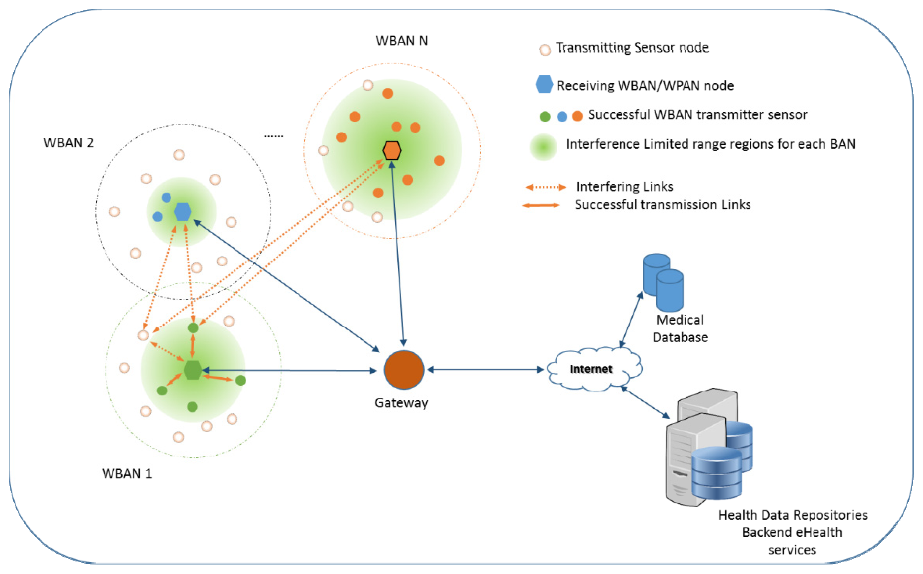
In this section, we describe the application scenario for biomedical telemetry wireless body/personal area networks. In our scenario the wireless biomedical networking ecosystem is formed by a collection of biomedical sensors, control/sink nodes and gateways (Figure 1). We assume that all medical related sensors are “light” in terms of computational resources and capable for wireless transmission of acquired medical data. These sensors are competing to gain access to a common medium and to transmit their data to a control/sink node forming wireless body/personal area networks. In the general case of our model we can easily assume that many such networks can co-exist in the same vicinity and thus we may have many competing transmission links operating simultaneously (from the same or different body/area personal networks).

The interference channel thus arises naturally in this situation and interference mitigation becomes critical for optimum network performance. In our previous work we compared the performance of a simplified network and found special cases of improvements in performance with transmission links operating concurrently [31].

In this study we use the Gaussian interference channel, where two point-to-point links with additive white Gaussian noise (AWGN) interfere with each other but in a more general setting where the interference channel refers to a network consisting of a number of transmitting and receiving nodes. A one to one correspondence between senders and receivers exists and each transmitter communicates only with its corresponding receiver, and each receiver is only interested in decoding the information from its corresponding transmitter. When many transmitter—receiver pairs share a wireless channel (common medium), each transmission is affected from the interference caused by all the other links and at the same time interferes with the operation of all other active links.

The network layer must be able to sense the amount of interference at a receiver, during the reception of a packet, and cope with it using power and/or rate adaptation (transmission rate adaptation can help maximize channel usage and power control can help lower the power consumption and interference). This can be accomplished using the Signal to Interference plus Noise Ratio (SINR) a performance metric that measures the ratio of the received signal power to the power of the undesired signals in the receiver. We calculate the Signal-to-Interference-plus-Noise ratio (SINR) at each receiver as the ratio of the power of the signal of interest (meaningful information of a link) to the combined power of the additive white Gaussian noise and the interference caused by the other active transmissions in range. Thus: $SIN{R}_{(i)}=\frac{P_i{G}_{ii}}{({\sum }_{j\ne i}{P}_j{G}_{ij})+n_i}$, where G_ij is the path loss from transmitter j to receiver i and is equal to ${\text{G}}_{\text{ij}}={(\lambda /4\hspace{0.17em}\pi )}^2·{\text{d}}_{(\text{i},\text{j})}^{-\text{a}}$, where λ is the wavelength, α is the path loss exponent and has typical values from 2 to 5, d_(i,j) is the distance between nodes i and j, and P_i is the transmitted power. White Gaussian noise is denoted as n_i. Another way of looking at the definition of the SINR, is to combine the transmission power of each transmitter with the quantity (λ/4π)² and consider P_i as the transmitted power at the distance of 1 meter and ${\text{G}}_{\text{ij}}={\text{d}}_{(\text{i},\text{j})}^{-\alpha }$. The product of P_iG_ii is the received power of interest for the signal for interest and ∑_j≠i P_jG_ij is the total interfering power of all other transmissions received at the receiver i. In the general case G_ij could be formulated to include fading effects, in this case it would have the expression ${\text{G}}_{\text{ij}}={(\lambda /4\hspace{0.17em}\pi )}^2·{\text{d}}_{(\text{i},\text{j})}^{-\text{a}}·f_{(i,j)}$, where f_(i,j) is the fading coefficient (a non-negative random variable).

A specific transmission i over a wireless link is considered successful when condition (1), known as the SINR criterion, is true for a given threshold value γ_(i) and for a positive vector P = (P₁, …, P_k) of transmission powers.

$$\frac{P_i{G}_{ii}}{\left({\sum }_{j\ne i}{P}_j{G}_{ij}\right)+n_i}\ge {\gamma }_{(i)}$$

(1)

For each transmission link i, the value of the SINR threshold γ_(i) depends on many design parameters and properties of the telecommunication system, such as the target BER, the modulation scheme, the error correction coding employed and the desired transmission bit-rate for each link. A set of simultaneous transmissions is considered successful when condition in Equation (1) is true for all the transmissions of this set. Given the telecommunication system and the application specific characteristics, each transmission might require different values for the SINR threshold γ for successful communication.

In this section we study the interference exhibited at the center of a circular networking area when interfering nodes (with equal transmitting power) are randomly distributed. Going a step further from previous works, we define the interference limited communication range (d_ILR) regions for biomedical body/personal area networks to be the critical communication region around a receiver, surrounded by a large number of randomly placed interfering nodes, within which if a transmitter is present, a successful communication link can be established. The value of d_ILR, as we will show, depends on a number of parameters: the number and the density of the surrounding interfering transmitters, the exclusion region around each receiver, the interference power level, and most importantly the selected transmission rate and mode of operation of the receiver.

We illustrate the generalized concept in Figure 1. The receivers of interest (pentagons) are placed at the center of the networking area, for each wireless body area network, around which many interfering transmitters are randomly deployed, belonging to the same or different wireless body/personal area networks. Given the amount of interference exhibited at the receiver’s site the interference limited communication range d_ILR is shown (the light green shaded disk). In this example the receiver acting as control/sink node in WBAN 1 experiences interference from all other transmitters deployed in the same vicinity (even if they belong to the same or different WBAN) transmitting simultaneously in the same channel. At the same time all the transmitters/sensors of WBAN 1 are causing interference to all other receivers. So only a portion of the sensors in WBAN 1 will be able to successfully transmit their data to the receiver of interest. These transmitters (colored circles) are located within this critical region d_ILR (shaded light green area around each receiver) inside which they can successfully communicate with the receiver of interest despite all the other interfering transmissions. The sensors/node that are not able to communicate are shown with uncolored dotted circles.

In the proposed model we make the approximation that interference behaves like white Gaussian noise which is equivalent to the applicability of the SINR criterion, and is equal to the sum of the received power, from all active transmitters I_i = (∑_j≠i P_jG_ij), at the receiver of interest i. P_j is the transmitted power and the path loss from transmitter j to receiver i is ${\text{G}}_{\text{ij}}={(\lambda /4\hspace{0.17em}\pi )}^2·{\pi }_{(\text{i},\text{j})}^{-\text{i}}=\text{D}·{\text{D}}_{(\text{i},\text{j})}^{-\text{i}}$, where λ is the wavelength, a is the path loss exponent and has typical values from 2 to 5 and d_(i,j) is the distance between nodes i and j. In the following sections we describe our approach for interference modeling when the transmitting nodes are positioned within the networking area using a random uniform distribution.

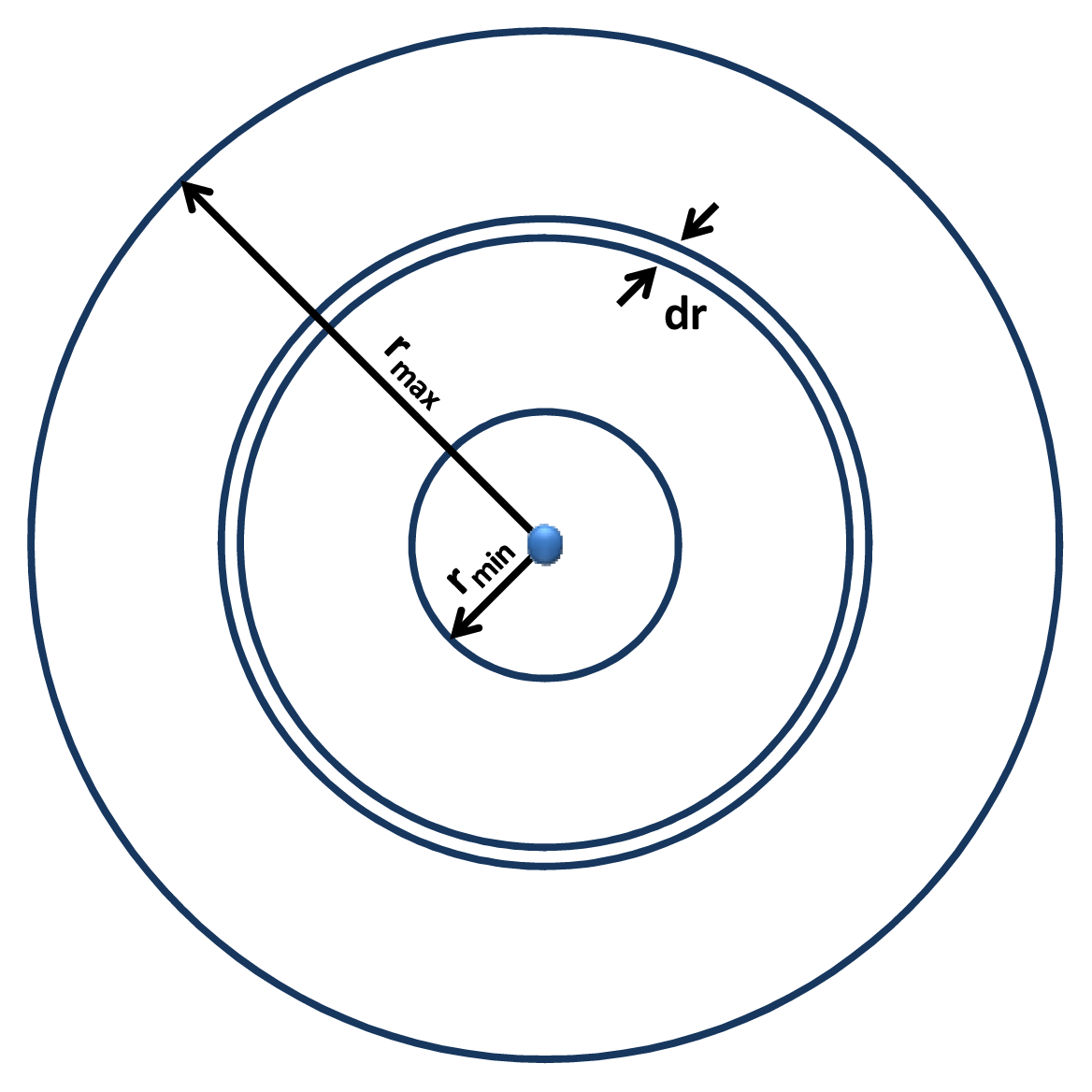
We assume, as illustrated in Figure 2, that a receiver of interest is placed at the center of each circular area and N_t transmitters-from all other wireless body/personal area networks, with equal transmission powers P, are placed randomly with uniform distribution inside an area bounded by the circles with radius r_max and r_min (r_min is the radius of the exclusion region around the receiver where no transmitters are allowed to operate).

Inside the ring from r to r + dr there are on average $\text{N}(\text{r})=\frac{{\text{N}}_{\text{t}}·2\pi rdr}{\pi (r_{max}^2-r_{min}^2)}=\left(\frac{2{\text{N}}_{\text{t}}\text{r}}{r_{max}^2-r_{min}^2}\right)\hspace{0.17em}dr$ transmitters causing interference with power equal to:

$$\text{I}(\text{r})=\sum _{\text{N}(\text{r})}{\text{P}}_{\text{j}}{\text{G}}_{\text{ij}}=\text{PD}\left(\frac{\left(\frac{2{\text{N}}_{\text{t}}\text{r}}{{\text{r}}_{\text{max}}^2-{\text{r}}_{\text{min}}^2}\right)}{{\text{r}}^{\text{a}}}\right)\hspace{0.17em}\text{dr}\Rightarrow \text{I}(\text{r})=\left(\frac{2{\text{PDN}}_{\text{t}}}{({\text{r}}_{\text{max}}^2-{\text{r}}_{\text{min}}^2)\hspace{0.17em}{\text{r}}^{\text{a}-1}}\right)\hspace{0.17em}\text{dr}$$

(2)

The total mean interference at the center of the circle then would be equal to:

$$\text{I}={\int }_{{\text{r}}_{\text{min}}}^{{\text{r}}_{\text{max}}}\left(\frac{2{\text{PDN}}_{\text{t}}}{({\text{r}}_{\text{max}}^2-{\text{r}}_{\text{min}}^2)\hspace{0.17em}{\text{r}}^{\text{a}-1}}\right)\hspace{0.17em}\text{dr}\Rightarrow \text{I}=\frac{2{\text{PDN}}_{\text{t}}}{{\text{r}}_{\text{max}}^2-{\text{r}}_{\text{min}}^2}{\int }_{{\text{r}}_{\text{min}}}^{{\text{r}}_{\text{max}}}\frac{\text{dr}}{{\text{r}}^{\text{a}-1}}$$

(3)

In [32] the authors performed a survey on wireless body communication and have found that the estimation of path loss exponent for body area wireless communication has be shown to be between 3 and 4, or in non-line-of-site situations the measured range is between 5 and 6. In a similar work in [33] the derived data are shown to be around 2.4 to 2.57 and 3.1 to 3.9. In our work thus to cover the general case we distinguish two different cases, for the calculation of the integral, depending on the path loss exponent a both of which we analyze below.

For path loss exponent a equal to 2 we get:

$$\text{I}=\frac{2{\text{PDN}}_{\text{t}}}{{\text{r}}_{\text{max}}^2-{\text{r}}_{\text{min}}^2}(\text{ln}\hspace{0.17em}{\text{r}}_{\text{max}}-\text{ln}\hspace{0.17em}{\text{r}}_{\text{min}})$$

(4)

where for r_max ≫ r_min we have $\text{I}\approx \frac{2{\text{PDN}}_{\text{t}}}{{\text{r}}_{\text{max}}^2}(\text{ln}\hspace{0.17em}{\text{r}}_{\text{max}}-\text{ax\hspace{0.17em}ln}\hspace{0.17em}{\text{r}}_{\text{min}})$, that is the interference has a strong dependence on r_max (and consequently on the transmitter density $\frac{{\text{N}}_{\text{t}}}{\pi {\text{r}}_{\text{max}}^2}$) and a much weaker (logarithmic) dependence on r_min (the size of the exclusion region).

For path loss exponent a greater than 2 we get:

$$\text{I}=\frac{2{\text{PDN}}_{\text{t}}}{(\text{a}-2)\hspace{0.17em}({\text{r}}_{\text{max}}^2-{\text{r}}_{\text{min}}^2)}\left(\frac{1}{{\text{r}}_{\text{min}}^{\text{a}-2}}-\frac{1}{{\text{r}}_{\text{max}}^{\text{a}-2}}\right)$$

(5)

where for r_max ≫ r_min we have: $\text{I}\approx \frac{2{\text{PDN}}_{\text{t}}}{(\text{a}-2)\hspace{0.17em}{\text{r}}_{\text{max}}^2}\left(\frac{1}{{\text{r}}_{\text{min}}^{\text{a}-2}}\right)$, the interference has a strong dependence on r_max (and consequently on the transmitter density $\frac{{\text{N}}_{\text{t}}}{\pi {\text{r}}_{\text{max}}^2}$) and polynomial dependence on r_min.

We distinguish two different cases, which are described below for realistic “real-world” links and Shannon capacity links.

2.1. Wireless System with Real-World Links

We consider the receiver at the center of the circular area to be part of a wireless network with “real-world” links that use a specific modulation scheme, a specific target BER and constant bandwidth. We assume the absence of any error control coding or any multiuser decoding scheme or any cooperation between transmitters and/or receivers and make the approximation that the interference behaves like white Gaussian noise, which combined with the thermal noise results in a combined total noise power spectral density N₀/2 in bandwidth BW. In this case there is a linear relationship between the achieved rate and the Signal to Interference plus Noise Ratio (SINR). We assume that the system’s bandwidth does not depend on the symbol duration of either the desired signal or the interfering signals. Thus the total power spectral density would be: $\frac{{\text{N}}_{\text{0}}}{2}=\frac{({\text{P}}_{\text{int}}+{\text{P}}_{\text{noise}})}{2\text{BW}}$ (where P_int and P_noise is the total power of interference and surrounding thermal noise respectively) and the energy per symbol for a link would be equal to E_s = P_iG_ii/R_s which results in an energy per symbol to interference-plus-noise density ratio equal to: $\frac{{\text{E}}_{\text{s}}}{{\text{N}}_{\text{0}}}=\frac{{\text{P}}_{\text{i}}{\text{G}}_{\text{ii}}}{({\sum }_{\text{j}\ne \text{i}}{\text{P}}_{\text{j}}{\text{G}}_{\text{ij}})+{\text{n}}_{\text{i}}}·\frac{\text{BW}}{{\text{R}}_{\text{s}}}$. As explained before if the SINR criterion is true for a given threshold value γ communication will be successful, and using the formulation from above we have: $\frac{{\text{P}}_{\text{i}}·\text{D}·{\text{d}}_{(\text{i},\text{i})}^{-\text{a}}}{\left({\sum }_{\text{j}\ne \text{i}}{\text{P}}_{\text{j}}·\text{D}·{\text{d}}_{(\text{i},\text{j})}^{-\text{a}}\right)+{\text{n}}_{\text{i}}}\ge \frac{{\text{E}}_{\text{s}}}{{\text{N}}_{\text{0}}}·\frac{{\text{R}}_{\text{b}}}{\text{k}·\text{BW}}$, where the white Gaussian noise is denoted by n_i and k = log₂M is the number of bits per symbol. The transmission bit rate is given by R_b = k·R_s and the values for the E_s/N₀ can be found from the Symbol Error Rate (SER) or BER requirements. Based on the interference calculation, as presented earlier, and assuming that (i) all transmitters in the area operate with transmission power P and that (ii) the interference power is much larger than the background noise (I ≫ n), we see that the “interference limited communication range” d_ILR, as defined above, is given by:

$$\begin{array}{c}{\text{d}}_{\text{ILR}}=\sqrt[\text{a}]{\frac{\frac{{\text{P}}_{\text{i}}·\text{D}}{\left({\sum }_{\text{j}\ne \text{i}}{\text{P}}_{\text{j}}·\text{D}·{\text{d}}_{(\text{i},\text{j})}^{-\text{a}}\right)+{\text{n}}_{\text{i}}}}{\frac{{\text{E}}_{\text{s}}}{{\text{N}}_{\text{0}}}·\frac{{\text{R}}_{\text{b}}}{\text{k}·\text{BW}}}}\approx \sqrt[\text{a}]{\frac{\frac{\text{P}·\text{D}}{\left({\sum }_{\text{j}\ne \text{i}}\text{P}·\text{D}·{\text{d}}_{(\text{i},\text{j})}^{-\text{a}}\right)}}{\frac{{\text{E}}_{\text{s}}}{{\text{N}}_{\text{0}}}·\frac{{\text{R}}_{\text{b}}}{\text{k}·\text{BW}}}}=\sqrt[\text{a}]{\frac{\frac{\text{PD}}{\text{I}}}{\frac{{\text{E}}_{\text{S}}}{{\text{N}}_{\text{0}}}·\frac{{\text{R}}_{\text{b}}}{\text{k}·\text{BW}}}}\\ \Rightarrow {\text{d}}_{\text{ILR}}=\sqrt[\text{a}]{\frac{\text{1}}{\frac{{\text{E}}_{\text{S}}}{{\text{N}}_{\text{0}}}·\frac{{\text{R}}_{\text{b}}}{\text{k}·\text{BW}}}·\frac{\text{PD}}{\text{I}}}\end{array}$$

(6)

Again we distinguish two cases:

$${\text{d}}_{\text{ILR}}=\{\begin{array}{l}\sqrt{\frac{1}{{\text{R}}_{\text{b}}{\text{N}}_{\text{t}}}}·\sqrt{\frac{\text{k}·\text{BW}}{2\frac{{\text{E}}_{\text{S}}}{{\text{N}}_{\text{0}}}}·\frac{({\text{r}}_{\text{max}}^2-{\text{r}}_{\text{min}}^2)}{(\text{ln}\hspace{0.17em}{\text{r}}_{\text{max}}-\text{ln}\hspace{0.17em}{\text{r}}_{\text{min}})}},\hspace{0.17em}\text{for}\hspace{0.17em}a=2\\ \sqrt[\text{a}]{\frac{1}{{\text{R}}_{\text{b}}{\text{N}}_{\text{t}}}}·\sqrt[\text{a}]{(\text{a}-2)·\frac{\text{k}·\text{BW}·({\text{r}}_{\text{max}}^2-{\text{r}}_{\text{min}}^2)}{2\frac{{\text{E}}_{\text{S}}}{{\text{N}}_{\text{0}}}\left(\frac{1}{{\text{r}}_{\text{min}}^{\text{a}-2}}-\frac{1}{{\text{r}}_{\text{max}}^{\text{a}-2}}\right)}},\hspace{0.17em}\text{for}\hspace{0.17em}a>2\end{array}$$

(7)(8)

In Figure 3 we see that the theoretical value of the d_ILR is a decreasing function of the number of interfering nodes and asymptotically falls to zero. When we have a high value for the path loss exponent (a > 2), we see that we obtain lower values for the d_ILR, when the number of transmitting nodes is relatively small. As N_t increases, the rate of convergence of d_ILR to zero is: ${(N_t)}^{-\frac{1}{2}}$ for a = 2 and ${(N_t)}^{-\frac{1}{a}}$ for a > 2.

2.2. Wireless System with Shannon Capacity Links

If the receiver of interest is part of a wireless network with Shannon capacity links, then R_b = BW · W i₂(1 + γ) and thus the SINR threshold γ, for R_b is equal to is $\gamma =2^{\frac{{\text{R}}_{\text{b}}}{\text{BW}}}-\text{W}$. Therefore the criterion for successful communication is: $\frac{{\text{P}}_{\text{i}}{\text{G}}_{\text{ii}}}{\left({\sum }_{\text{j}\ne \text{i}}{\text{P}}_{\text{j}}{\text{G}}_{\text{ij}}\right)+{\text{n}}_{\text{i}}}\ge 2^{\frac{{\text{R}}_{\text{b}}}{\text{BW}}}-\text{W}$. Following the analysis presented before, and taking into account the interference calculations and the criterion for successful communication in this case the interference limited communication region is given by:

$$\begin{array}{c}{\text{d}}_{\text{ILR}}=\sqrt[\text{a}]{\frac{1}{2^{\frac{{\text{R}}_{\text{b}}}{\text{BW}}}-1}·\frac{{\text{P}}_{\text{i}}·\text{D}}{\left({\sum }_{\text{j}\ne \text{i}}{\text{P}}_{\text{j}}·\text{D}·{\text{d}}_{(\text{i},\text{j})}^{-\text{a}}\right)+{\text{n}}_{\text{i}}}}\approx \sqrt[\text{a}]{\frac{1}{2^{\frac{{\text{R}}_{\text{b}}}{\text{BW}}}-1}·\frac{\text{P}·\text{D}}{\left({\sum }_{\text{j}\ne \text{i}}\text{P}·\text{D}·{\text{d}}_{(\text{i},\text{j})}^{-\text{a}}\right)}}\\ \Rightarrow {\text{d}}_{\text{ILR}}=\sqrt[\text{a}]{\frac{1}{2^{\frac{{\text{R}}_{\text{b}}}{\text{BW}}}-1}·\frac{\text{PD}}{\text{I}}}\end{array}$$

(9)

We distinguish two cases:

$${\text{d}}_{\text{ILR}}=\{\begin{array}{l}\sqrt{\frac{{\text{r}}_{\text{max}}^2-{\text{r}}_{\text{min}}^2}{2(\text{ln}\hspace{0.17em}{\text{r}}_{\text{max}}-\text{ln}\hspace{0.17em}{\text{r}}_{\text{min}})}·}\sqrt{\frac{1}{2^{\frac{{\text{R}}_{\text{b}}}{\text{BW}}}-1}·\frac{1}{{\text{N}}_{\text{t}}}},\hspace{0.17em}\text{for}\hspace{0.17em}a=2\\ \sqrt[\text{a}]{\frac{1}{2^{\frac{{\text{R}}_{\text{b}}}{\text{BW}}}-1}·\frac{1}{{\text{N}}_{\text{t}}}·\frac{(\text{a}-2)\hspace{0.17em}({\text{r}}_{\text{max}}^2-{\text{r}}_{\text{min}}^2)}{2\left(\frac{1}{{\text{r}}_{\text{min}}^{\text{a}-2}}-\frac{1}{{\text{r}}_{\text{max}}^{\text{a}-2}}\right)}},\hspace{0.17em}\text{for}\hspace{0.17em}a>2\end{array}$$

(10)(11)

Figure 4 shows that the d_ILR has the same behavior as before (Figure 3) but its values are much higher (as expected because of the much better performance of the link). For small number of transmitters the d_ILR with a = 2 is larger than the d_ILR with a > 2. The rate of convergence to zero is the same as before.

3. Results and Discussion

In order to validate our theoretical estimations, for the computation of the interference values and the interference limited communication range, we implemented extensive Monte-Carlo simulations [34] using the network model presented above. The parameters for our simulation are chosen to reflect the description of our system model (Figure 1) for a general-purpose wireless biomedical network used as the medium to transfer different bio-signals. In this scenario we may have many biomedical sensors, control/sink nodes and gateways each one operating in proximity of each other forming different wireless body/personal area networks.

3.1. Interference Measurements

Our interference simulation experiments are presented in Figure 5. We compare our simulation results with the theoretical values calculated using Equations (4) and (5). The number of the interfering nodes increases from 1 to 100. All nodes are randomly placed (using uniform distribution) inside a circular area bounded by the circles with r_min and r_max = 100 m. The receiver of interest is positioned at the center of the area where the highest amount of interference is exhibited. The transmission power is assumed the same for all transmitting nodes and is equal to 1mW. In the simulations we calculate the distance of each transmitting node from the center of the networking area where the receiver of interest is located. Path losses due to fading and shadowing are not considered. The path loss exponent a varies from 2 (free space) to 4 [35]. The channel bandwidth is assumed constant and equal to 10⁷Hz and all transmitting nodes employ a BPSK modulation scheme (thus k in Equations (7) and (8) is equal to 1).

The results from the proposed theoretical model are in a very good agreement with the values of the mean interference levels obtained by simulations. Figure 5a shows the effect of the path loss exponent on interference and Figure 5b shows the effect of r_min (the distance around the receiver where a transmitter cannot be placed, i.e., the exclusion region). As expected a higher value for the path loss exponent results in lower levels of interference, and a larger r_min leads to lower interference.

In Figure 6, we present the mean interference levels, using simulations, for path loss exponent equal to 2 and 4 (plot (a) and plot (b), respectively) when we relax our assumption on the receiver’s position and assume that it is placed at distance (x) from the center of the networking area, where the offset x ∈ [0, r_max]. When a receiver is close to the borders of the networking area the interference level decreases. This given that the number of the nearby interfering transmitters decreases near the borders, is natural since the separation distance of interfering transmitters becomes larger than r_max and thus their interference diminishes.

The difference, between the interference levels at the center of the networking area, calculated with Equations (4) and (5), and at a quite large offset from the center is remarkably small as is evident in Figure 6. In fact the approximation is quite good with even a 60% or 70% (for a = 2) and 90% (for a = 4) offset from the center of the circle.

The interference level on the border of the circular area (100% offset) is approximately half of the level at the center. Therefore we can assume that, for the largest part of the networking area, the interference level as given by Equations (4) and (5) is a quite accurate approximation. The same holds true for the values of the d_ILR, given by Equations (7) and (8). If more accuracy is desired it is possible to calculate the interference at any offset (x) using the method described in [24], but in this case a much more complicated analysis would be required.

3.2. Interference Limited Communication Range Regions

In this section we present our simulation results for the d_ILR which is the maximum distance from which a transmitter can successfully send data to the centrally positioned receiver with a specific rate. We compare our simulation results with the results from calculations based on the theoretical analysis presented previously.

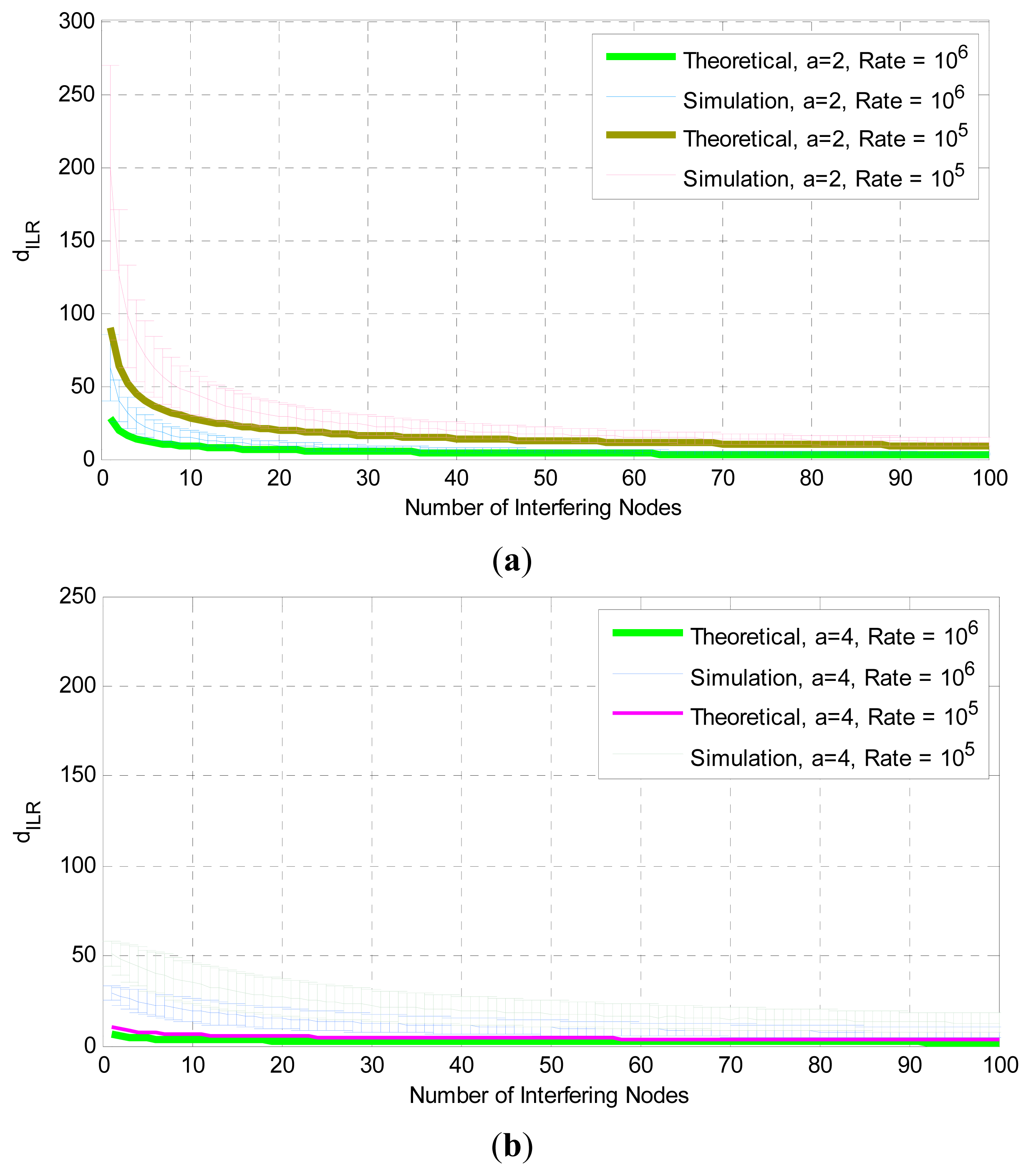
Figure 7 illustrates, the mean interference limited communication range with the confidence intervals (standard deviation) versus the number of interfering nodes, using different transmission data rates, r_min = 0.4 m and path loss exponent equal to 2 and 4 in plots (a) and (b) respectively. By adapting the transmission rate (lowering in this case) we can control the size of the region (enlarge it) and allow more transmitters to be able to successfully communicate with the receiver of interest. This result implies that we can use an upper layer communication parameter to easily adapt (using the proposed method) to the experienced interference. The theoretical and simulation results are in better agreement as the number of interfering nodes increases. We can see that using a higher path loss exponent assumption reveals how much the exhibited interference affect communication and that is the reason that the region is restricted to smaller sizes. We observe (Figure 7) that the theoretical calculations give a lower value (worst case scenario) but are within the deviation interval of the simulation results, for a = 2 (plot (a)), but not for a = 4 (plot (b)). The reason of this discrepancy lies in the way we use the interference measurements to calculate d_ILR.

A different approach for measuring the value of d_ILR, is to first measure the mean interference level, repeating the experiment (random placement of transmitting nodes) a large number of times, and then compute the d_ILR using this mean value of interference. In this case (Figure 8) the results are in accordance with the ones found from the theoretical calculations. This corresponds to a situation where a receiving node monitors the varying (due to changes in the network) interference for a period of time and calculates the mean interference levels in order to find the d_ILR.

In the final set of simulations the procedure described at the beginning of this section is employed (we measure the value of the d_ILR for each placement of the transmitting nodes and then calculate its mean value).

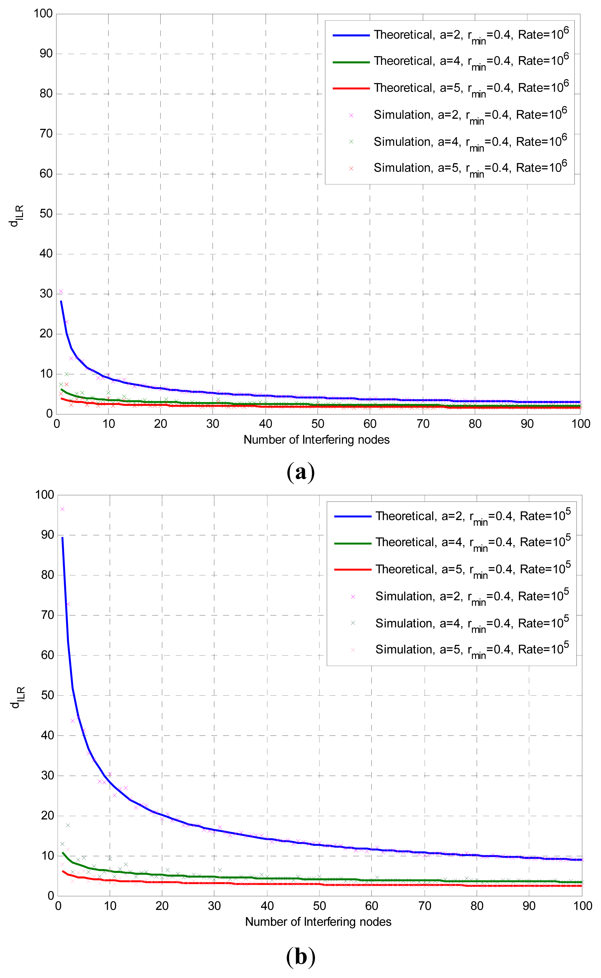
Changing the distance r_min (exclusion region) the interference limited communication range is not significantly affected, as shown in Figure 9. As was noted before, for a higher path loss exponent there is a discrepancy between the simulation and calculation results for the d_ILR, which is reduced as the number of interfering nodes increases. This agrees with the results presented in [24] where it is noted that for small number of interfering nodes the theoretical and simulation results don’t seem to converge. In the same figure we can see that for path loss exponent a = 4 the calculated d_ILR values are smaller than those for a = 2.

Finally, we compare the calculated values of the mean interference limited communication region and the results from our simulations, for path loss exponent equal to 2 and 4, Figure 10 plots (a) and (b) respectively, when we relax our assumption on the receiver’s position and assume a specific offset x from the center of the networking area, where x ∈ [0, r_max], as we have done previously for the interference study. We can see that when the receiving node moves to the border of the networking area the value of the d_ILR is increasing (since the interference is decreasing), but it remains very close to its value at the center for a 60% or 70% (for a = 2) and for a 80% or 90% (for a = 4) offset from the center of the circle. The calculated values (black line) are always smaller than the simulation results; that is, they correspond to a worst-case scenario.

4. Conclusions

Interference suppression in biomedical wireless medical networks is a critical issue that would allow successful and reliable communication in critical medical data networking environments. In this paper we presented a detailed analysis on interference calculation for a receiving node placed in the vicinity of the center of a networking area when interfering transmitters are randomly placed around it using a uniform distribution. Our results indicate ways to compensate the degree of interference exhibited in each receiver with respect to network topology, transmission rate and individual maximum power constrains of each transmitter. The presented theoretical analysis provides a very good approximation of the mean interference found via simulations. We extended previous works by introducing the interference limited communication range (d_ILR) as the critical region around a receiver within which a transmitter, despite the presence of the other interfering nodes, can successfully send its data to the receiver of interest with a specific rate. We verified our results with simulations and presented the rate of convergence of the interference-limited region for wireless biomedical networks. Finally, we validated the accuracy of our model even when we relax our assumptions on the receiver’s position in respect with the interfering transmitters. No matter the receiver’s position, within a wireless biomedical area network, our model remains valid.

References

- Breen, G.-M.; Matusitz, J. An Evolutionary Examination of Telemedicine: A Health and Computer-Mediated Communication Perspective. Soc. Work Public Health 2010, 25, 59–71. [Google Scholar]
- Galarraga, M.; Serrano, L.; Martinez, I.; de Toledo, P.; Reynolds, M. Telemonitoring Systems Interoperability Challenge: An Updated Review of the Applicability of ISO/IEEE 11073 Standards for Interoperability in Telemonitoring. Proceedings of the 29th Annual International Conference of the IEEE Engineering in Medicine and Biology Society, Lyon, France, 23–26 August 2007; pp. 6161–6165.
- Abreu, C.; Mendes, P. Wireless sensor networks for biomedical applications. Proceedings of the 2013 IEEE 3rd Portuguese Meeting in Bioengineering (ENBENG), Braga, Portugal, 20–23 February 2013; pp. 1–4.
- Lozano, C.A.; Tellez, C.E.; Rodriguez, O.J. Biosignal Monitoring Using Wireless Sensor Networks. In Biomedical Engineering, Trends in Electronics, Communications and Software; Laskovski, A.N., Ed.; InTech: Rijeka, Croatia, 2011. [Google Scholar]
- Hristoskova, A.; Sakkalis, V.; Zacharioudakis, G.; Tsiknakis, M.; de Turck, F. Ontology-Driven Monitoring of Patient’s Vital Signs Enabling Personalized Medical Detection and Alert. Sensors 2014, 14, 1598–1628. [Google Scholar]
- Kartakis, S.; Sakkalis, V.; Tourlakis, P.; Zacharioudakis, G.; Stephanidis, C. Enhancing Health Care Delivery through Ambient Intelligence Applications. Sensors 2012, 12, 11435–11450. [Google Scholar]
- Sakkalis, V. Applied strategies towards EEG/MEG biomarker identification in clinical and cognitive research. Biomark. Med 2011, 5, 93–105. [Google Scholar]
- Pelegris, P.; Banitsas, K.; Orbach, T.; Marias, K. A novel method to detect Heart Beat Rate using a mobile phone. Proceedings of the 2010 Annual International Conference of the IEEE Engineering in Medicine and Biology Society (EMBC), Buenos Aires, Argentina, 31 August–4 September 2010; pp. 5488–5491.
- Meystre, S. The Current State of Telemonitoring: A Comment on the Literature Telemedicine and e-Health. Telemed. e-Health 2005, 11, 63–69. [Google Scholar]
- Choi, J.S.; Zhou, M. Recent Advances in Wireless Sensor Networks for Health Monitoring. Int. J. Intell. Control Syst 2010, 15, 49–58. [Google Scholar]
- Smith, D.; Miniutti, D.; Lamahewa, T.; Hanlen, L. Propagation Models for Body Area Networks: A Survey and New Outlook. IEEE Antennas Propag. Mag 2010, 55, 97–117. [Google Scholar]
- Javaid, N.; Khan, N.A.; Shakir, M.; Khan, M.A.; Bouk, S.H.; Khan, Z.A. Ubiquitous HealthCare in Wireless Body Area Networks—A Survey. 2013. arXiv:1303.2062[cs.NI]. [Google Scholar]
- Phunchongharn, P.; Niyato, D.; Hossain, E.; Camorlinga, S. An EMI-Aware Prioritized Wireless Access Scheme for e-Health Applications in Hospital Environments. IEEE Trans. Inf. Technol. Biomed 2010, 14, 1247–1258. [Google Scholar]
- Joshi, G.P.; Nam, S.Y.; Kim, S.W. Cognitive Radio Wireless Sensor Networks: Applications, Challenges and Research Trends. Sensors 2013, 13, 11196–11228. [Google Scholar]
- Chiarugi, F.; Trypakis, D.; Spanakis, E.G. Problems and Solutions for Storing and Sharing Data from Medical Devices in eHealth Applications. Proceedings of 2nd OpenECG Workshop, Berlin, Germany, 1–3 April 2004; pp. 65–69.
- Spanakis, E.G.; Chiarugi, F.; Kouroubali, A.; Spat, S.; Beck, B.; Asanin, S.; Rosengren, P.; Gergely, G.T.; Thestrup, J. Diabetes Management Using Modern Information and Communication Technologies and New Care Models. Interact. J. Med. Res 2012, 1, e8. [Google Scholar]
- Spanakis, E.G.; Lelis, P.; Chiarugi, F.; Chronaki, C.; Tsiknakis, M. R&D challenges in developing an ambient intelligence eHealth platform. Proceedings of 3rd European Medical & Biological Engineering Conference (EMBEC’05), Prague, Czech Republic, 20–25 November 2005; 11, pp. 1727–1983.
- Spat, S.; Höll, B.; Beck, B.; Chiarugi, F.; Kontogiannis, V.; Spanakis, E.G.; Manousos, D.; Pieber, T. A Mobile Android-based Application for in-hospital Glucose Management in compliance with the Medical Device Directive for Software. Proceedings of the 2nd International ICST Conference on Wireless Mobile Communication and Healthcare (MobiHealth 2011), Kos Island, Greece, 5–7 October 2011.
- Spanakis, E.G.; Voyiatzis, A.G. DAPHNE: A Disruption-Tolerant Application Proxy for e-Health Network Environments. Proceedings of the 3rd International Conference on Wireless Mobile Communication and Healthcare, Paris, France, 21–23 November 2012.
- Traganitis, A.P.; Spanakis, E.G.; Orphanoudakis, S.C. Wireless Communication Technologies for Mobile Healthcare Applications: Experiences and Evaluation of Security Related Issues. In M-Health: Emerging Mobile Health Systems; Springer: New York, NY, USA; pp. 65–80.
- Shakkottai, S.; Rappaport, T.S.; Karlsson, P.C. Cross-layer design for wireless networks. IEEE Commun. Mag 2003, 41, 74–80. [Google Scholar]
- Charafeddine, M.; Sezgin, A.; Paulrajm, A. Rate Region Frontiers for n-user Interference Channel with Interference as Noise. Proceedings of the 45th Annual Allerton Conference on Communication, Control, and Computing, Monticello, IL, USA, 26–28 September 2007.
- Hekmat, R.; van Mieghem, P. Interference in Wireless Multi-Hop Ad-Hoc Networks and Its Effect on Network Capacity. Wirel. Netw 2004, 10, 389–399. [Google Scholar]
- Cardieri, P. Modeling Interference in Wireless Ad Hoc Networks. IEEE Commun. Surv. Tutor 2010, 12, 551–572. [Google Scholar]
- De Moraes, R.M.; Garcia-Luna-Aceves, J.J.; Sadjadpour, H.R. Many-to-many communication for mobile ad hoc networks. IEEE Trans. Wirel. Commun 2009, 8, 2388–2399. [Google Scholar]
- Pappas, N.; Kountouris, M.; Ephremides, A. The stability region of the two-user interference channel. Proceedings of the IEEE Information Theory Workshop (ITW), Sevilla, Spain, 9–13 September 2013. [CrossRef]
- Annapureddy, V.S.; Veeravalli, V.V. Gaussian Interference Networks: Sum Capacity in the Low-Interference Regime and New Outer Bounds on the Capacity Region. IEEE Trans. Inf. Theory 2009, 55, 3032–3050. [Google Scholar]
- Carleial, A. A case where interference does not reduce capacity (Corresp.). IEEE Trans. Inf. Theory 1975, 21, 569–570. [Google Scholar]
- Gupta, P.; Kumar, P.R. The capacity of wireless networks. IEEE Trans. Inf. Theory 2000, 46, 388–404. [Google Scholar]
- Rekha, M.; Buehrer, R.M.; Jeffrey, H.R. Impact of Exclusion Region and Spreading in Spectrum-sharing Ad hoc Networks. Proceedings of the First International Workshop on Technology and Policy for Accessing Spectrum (TAPAS 06) ACM, Boston, MA, USA, 5 August 2006.
- Spanakis, E.G.; Traganitis, A.P.; Ephremides, A. Rate Region and Power Considerations in a simple 2 × 2 Interference Channel. Proceedings of the IEEE Information Theory Workshop on Networking and Information Theory, ITW 2009, Volos, Greece, 10–12 June 2009.
- Latré, B.; Braem, B.; Moerman, I.; Blondia, C.; Demeester, P. A survey on wireless body area networks. Wirel. Netw 2011, 17. [Google Scholar] [CrossRef]
- Guraliuc, A.; Serra, A.A.; Nepa, P.; Manara, G.; Potorti, F.; Barsocchi, P. Body posture/activity detection: Path loss characterization for 2.4 GHz on-body wireless sensors. Proceedings of the IEEE Antennas and Propagation Society International Symposium, APSURSI 2009, Charleston, SC, USA, 1–5 June 2009; pp. 1–4.
- Robert, C.P.; Casella, G. Monte Carlo Statistical Methods; Springer: Berlin, Germany, 2004. [Google Scholar]
- Rappaport, T.S. Wireless Communications, Principles and Practice; Prentice Hall PTR: Upper Saddle River, NJ, USA, 2002. [Google Scholar]
© 2014 by the authors; licensee MDPI, Basel, Switzerland This article is an open access article distributed under the terms and conditions of the Creative Commons Attribution license (http://creativecommons.org/licenses/by/3.0/).
Share and Cite
Spanakis, E.G.; Sakkalis, V.; Marias, K.; Traganitis, A. Cross Layer Interference Management in Wireless Biomedical Networks. Entropy 2014, 16, 2085-2104. https://0-doi-org.brum.beds.ac.uk/10.3390/e16042085
Spanakis EG, Sakkalis V, Marias K, Traganitis A. Cross Layer Interference Management in Wireless Biomedical Networks. Entropy. 2014; 16(4):2085-2104. https://0-doi-org.brum.beds.ac.uk/10.3390/e16042085
Chicago/Turabian StyleSpanakis, Emmanouil G., Vangelis Sakkalis, Kostas Marias, and Apostolos Traganitis. 2014. "Cross Layer Interference Management in Wireless Biomedical Networks" Entropy 16, no. 4: 2085-2104. https://0-doi-org.brum.beds.ac.uk/10.3390/e16042085