F-Geometry and Amari’s α-Geometry on a Statistical Manifold

Abstract

In this paper, we introduce a geometry called F-geometry on a statistical manifold S using an embedding F of S into the space ℝ_X of random variables. Amari’s α−geometry is a special case of F −geometry. Then using the embedding F and a positive smooth function G, we introduce (F, G)−metric and (F, G)−connections that enable one to consider weighted Fisher information metric and weighted connections. The necessary and sufficient condition for two (F, G)−connections to be dual with respect to the (F, G)−metric is obtained. Then we show that Amari’s 0−connection is the only self dual F −connection with respect to the Fisher information metric. Invariance properties of the geometric structures are discussed, which proved that Amari’s α−connections are the only F −connections that are invariant under smooth one-to-one transformations of the random variables.

1. Introduction

Geometric study of statistical estimation has opened up an interesting new area called the Information Geometry. Information geometry achieved a remarkable progress through the works of Amari [1,2], and his colleagues [3,4]. In the last few years, many authors have considerably contributed in this area [5–9]. Information geometry has a wide variety of applications in other areas of engineering and science, such as neural networks, machine learning, biology, mathematical finance, control system theory, quantum systems, statistical mechanics, etc.

A statistical manifold of probability distributions is equipped with a Riemannian metric and a pair of dual affine connections [2,4,9]. It was Rao [10] who introduced the idea of using Fisher information as a Riemannian metric in the manifold of probability distributions. Chentsov [11] introduced a family of affine connections on a statistical manifold defined on finite sets. Amari [2] introduced a family of affine connections called α−connections using a one parameter family of functions, the α−embeddings. These α−connections are equivalent to those defined by Chentsov. The Fisher information metric and these affine connections are characterized by invariance with respect to the sufficient statistic [4,12] and play a vital role in the theory of statistical estimation. Zhang [13] generalized Amari’s α−representation and using this general representation together with a convex function he defined a family of divergence functions from the point of view of representational and referential duality. The Riemannian metric and dual connections are defined using these divergence functions.

In this paper, Amari’s idea of using α−embeddings to define geometric structures is extended to a general embedding. This paper is organized as follows. In Section 2, we define an affine connection called F −connection and a Riemannian metric called F −metric using a general embedding F of a statistical manifold S into the space of random variables. We show that F −metric is the Fisher information metric and Amari’s α−geometry is a special case of F −geometry. Further, we introduce (F, G)−metric and (F, G)−connections using the embedding F and a positive smooth function G.

In Section 3, a necessary and sufficient condition for two (F, G)−connections to be dual with respect to the (F, G)−metric is derived and we prove that Amari’s 0−connection is the only self dual F −connection with respect to the Fisher information metric. Then we prove that the set of all positive finite measures on X, for a finite X, has an F −affine manifold structure for any embedding F. In Section 4, invariance properties of the geometric structures are discussed. We prove that the Fisher information metric and Amari’s α−connections are invariant under both the transformation of the parameter and the transformation of the random variable. Further we show that Amari’s α−connections are the only F −connections that are invariant under both the transformation of the parameter and the transformation of the random variable.

Let (X, B) be a measurable space, where X is a non-empty subset of ℝ and B is the σ-field of subsets of X. Let ℝ_X be the space of all real valued measurable functions defined on (X, B). Consider an n−dimensional statistical manifold S = {p(x; ξ) / ξ = [ξ¹, …, ξⁿ] ∈ $\mathbb{E}$ ⊆ ℝⁿ}, with coordinates ξ = [ξ¹, …, ξⁿ], defined on X. S is a subset of P(X), the set of all probability measures on X given by

$$P(X):=\{p:X\to ℝ/p(x)>0(\forall x\in X);{\displaystyle \underset{X}{\int }p(x)dx=1}\}.$$

(1)

The tangent space to S at a point p_ξ is given by

$$T_{\xi }(S)=\{{\displaystyle \sum _{i=1}^n{\alpha }^i{\partial }_i/{\alpha }^i\in ℝ\}\text{where }{\partial }_i=\frac{\partial }{\partial {\xi }^i}}.$$

(2)

Define ℓ (x; ξ) = log p(x; ξ) and consider the partial derivatives $\{\frac{\partial \ell }{\partial {\xi }^i}={\partial }_i\ell ;i=1,\dots .,n\}$ which are called scores. For the statistical manifold S, ∂_il’s are linearly independent functions in x for a fixed ξ. Let $T_{\xi }^1(S)$ be the n-dimensional vector space spanned by n functions {∂_iℓ; i = 1, …., n in x. So

$$T_{\xi }^1(S)=\{\underset{i=1}{\overset{n}{{{{\displaystyle \sum }}^{\text{}}}^{\text{}}}}{A}^i{\partial }_i\ell /A^i\in ℝ\}.$$

(3)

Then there is a natural isomorphism between these two vector spaces T_ξ(S) and $T_{\xi }^1(S)$ given by

$${\partial }_i\in T_{\xi }(S)\leftrightarrow {\partial }_i\ell (x;\xi )\in T_{\xi }^1(S).$$

(4)

Obviously, a tangent vector $A={\displaystyle {\sum }_{i=1}^n{A}^i{\partial }_i\in T_{\xi }(S)}$ corresponds to a random variable $A(x)={\displaystyle {\sum }_{i=1}^n{A}^i{\partial }_i\ell (x;\xi )\in T_{\xi }^1(S)}$ having the same components Aⁱ. Note that T_ξ(S) is the differentiation operator representation of the tangent space, while $T_{\xi }^1(S)$ is the random variable representation of the same tangent space. The space $T_{\xi }^1(S)$ is called the 1-representation of the tangent space. Let A and B be two tangent vectors in T_ξ(S) and A(x) and B(x) be the 1–representations of A and B respectively. We can define an inner product on each tangent space T_ξ(S) by

$$g_{\xi }(A,B)=<A,B{>}_{\xi }=E_{\xi }[A(x)B(x)]=\int A(x)B(x)p(x;\xi )dx.$$

(5)

Especially the inner product of the basis vectors ∂_i and ∂_j is

$$g_{ij}(\xi )=<{\partial }_i,{\partial }_i{>}_{\xi }=E_{\xi }[{\partial }_i\ell {\partial }_j\ell ]=\int {\partial }_i\ell (x;\xi ){\partial }_j\ell (x;\xi )p(x;\xi )dx.$$

(6)

Note that g = <, > defines a Riemannian metric on S called the Fisher information metric. On the Riemannian manifold (S, g =<, >), define n³ functions Γ_ijk by

$${\mathrm{\Gamma }}_{ijk}(\xi )=E_{\xi }[{\partial }_i{\partial }_j\ell (x;\xi ))({\partial }_k\ell (x;\xi ))].$$

(7)

These functions Γ_ijk uniquely determine an affine connection ∇ on S by

$${\mathrm{\Gamma }}_{ijk}(\xi )=<{\nabla }_{{\partial }_i}{\partial }_j,{\partial }_k>\xi .$$

(8)

∇ is called the 1−connection or the exponential connection.

Amari [2] defined a one parameter family of functions called the α−embeddings given by

$$L_{\alpha }(p)=\{\begin{array}{cc}\frac{2}{1-\alpha }{p}^{\frac{1-\alpha }{2}}& \alpha \ne 1\\ \text{log}p& \alpha =1\end{array}$$

(9)

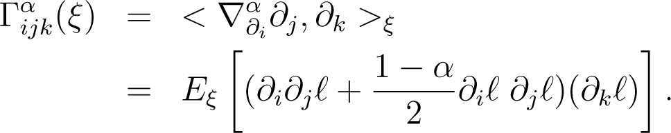
Using these, we can define n³ functions ${\mathrm{\Gamma }}_{ijk}^{\alpha }$ by

$${\mathrm{\Gamma }}_{ijk}^{\alpha }=\int {\partial }_i{\partial }_j{L}_{\alpha }(p(x;\xi )){\partial }_k{L}_{-\alpha }(p(x;\xi ))dx$$

(10)

These ${\mathrm{\Gamma }}_{ijk}^{\alpha }$ uniquely determine affine connections ∇^α on the statistical manifold S by

$${\mathrm{\Gamma }}_{ijk}^{\alpha }=<{\nabla }_{{\partial }_i}^{\alpha }{\partial }_j,{\partial }_k>$$

(11)

which are called α−connections.

2. F−Geometry of a Statistical Manifold

On a statistical manifold S, the Fisher information metric and exponential connection are defined using the log embedding. In a similar way, α−connections are defined using a one parameter family of functions, the α−embeddings. In general, we can give other geometric structures on S using different embeddings of the manifold S into the space of random variables ℝ_X.

Let F: (0, ∞) → ℝ be an injective function that is at least twice differentiable. Thus we have F′(u) ≠ 0, ∀ u ∈ (0, ∞). F is an embedding of S into ℝ_X that takes each p(x; ξ) → F (p(x; ξ)). Denote F (p(x; ξ)) by F (x; ξ) and ∂_iF can be written as

$${\partial }_{i}F(x;\xi )=p(x;\xi )F^{\prime }(p(x;\xi )){\partial }_i\ell (p(x;\xi )).$$

(12)

It is clear that ∂_iF (x; ξ); i = 1, …, n are linearly independent functions in x for fixed ξ since ∂_i℞(p(x; ξ)); i = 1, …, n are linearly independent. Let $T_{F(p_{\xi })}$ F (S) be the n-dimensional vector space spanned by n functions ∂_iF; i = 1, …., n in x for fixed ξ. So

$$T_{F(p_{\xi })}F(S)=\{{\displaystyle \sum _{i=1}^n{A}^i{\partial }_{i}F/A^i\in ℝ\}}$$

(13)

Let the tangent space $T_{F(p_{\xi })}$ (F (S)) to F (S) at the point F(p_ξ) be denoted by $T_{\xi }^F(S)$. There is a natural isomorphism between the two vector spaces T_ξ(S) and $T_{\xi }^F(S)$ given by

$${\partial }_i\in T_{\xi }(S)\leftrightarrow {\partial }_{i}F(x;\xi )\in T_{\xi }^F(S).$$

(14)

$T_{\xi }^F(S)$ is called the F−representation of the tangent space T_ξ(S).

For any $A={\displaystyle {\sum }_{i=1}^n{A}^i{\partial }_i\in T_{\xi }(S)}$, the corresponding $A(x)={\displaystyle {\sum }_{i=1}^n{A}^i{\partial }_{i}F\in T_{\xi }^F(S)}$ is called the F–representation of the tangent vector A and is denoted by A^F(x). Note that $T_{\xi }^F(S)\subseteq T_{F(p_{\xi })}({ℝ}_X)$. Since ℝ_X is a vector space, its tangent space $T_{F(p_{\xi })}({ℝ}_X)$ can be identified with ℝ_X. So $T_{\xi }^F(S)\subseteq ({ℝ}_X)$.

Definition 2.1

F−expectation of a random variable f with respect to the distribution p(x; ξ) is defined as

$$E_{\xi }^F(f)=\int f(x)\frac{1}{p{(F^{\prime }(p))}^2}dx.$$

(15)

We can use this F−expectation to define an inner product in ℝ_X by

$$<f,g{>}_{\xi }^F=E_{\xi }^F[f(x)g(x)],$$

(16)

which induces an inner product on T_ξ(S) by

$$<A,B{>}_{\xi }^F=E_{\xi }^F[A^F(x)B^F(x)];A,B\in T_{\xi }(S).$$

(17)

Proposition 2.2

The induced metric <, >^F on S is the Fisher information metric g =<, > on S.

Proof

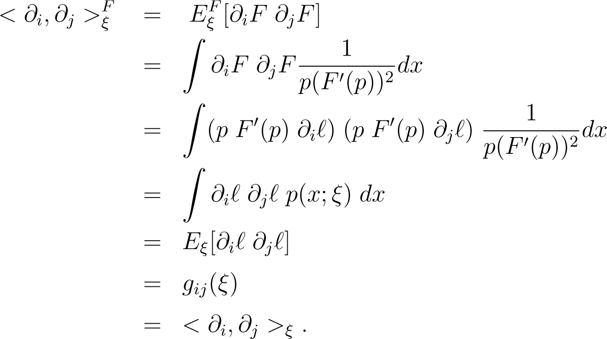
For any basis vectors ∂_i, ∂_j ∈ T_ξ(S)

(18)

So the metric <, >^F on S induced by the embedding F of S into ℝ_X is the Fisher information metric g =<, > on S.

We can induce a connection on S using the embedding F.

Let ${\pi }_{|p_{\xi }}^F:{ℝ}_X\to T_{\xi }^F(S)$ be the projection map.

Definition 2.3

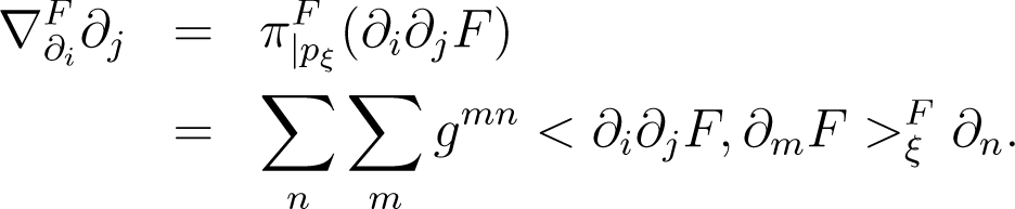
The connection induced by the embedding F on S, the F−connection, is defined as

(19)

where [g^mn(ξ)] is the inverse of the Fisher information matrix G(ξ) = [g_mn(ξ)]. Note that the F−connections are symmetric.

Lemma 2.4

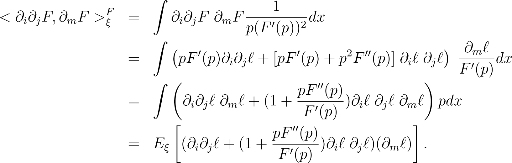
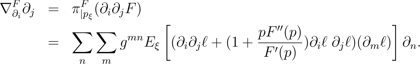
The F −connection and its components can be written in terms of scores as

$${\nabla }_{{\partial }_i}^F{\partial }_j={\displaystyle \sum _n{\displaystyle \sum _m{g}^{mm}{E}_{\xi }\left[({\partial }_i{\partial }_j\ell +(1+\frac{p{F}^{″}(p)}{F^{\prime }(p)}){\partial }_i\ell {\partial }_i\ell )({\partial }_m\ell )\right]}{\partial }_n}$$

(20)

and

$${\mathrm{\Gamma }}_{ijk}^F(\xi )=E_{\xi }\left[({\partial }_i{\partial }_j\ell +(1+\frac{p{F}^{″}(p)}{F^{\prime }(p)}){\partial }_i\ell {\partial }_i\ell )({\partial }_k\ell )\right]$$

(21)

Proof

From Equation (12), we have

$${\partial }_i{\partial }_{j}F=p{F}^{\prime }(p){\partial }_i{\partial }_j\ell +[p{F}^{\prime }(p)+p^2{F}^{″}(p)]{\partial }_i\ell {\partial }_j\ell .$$

(22)

Therefore

(23)

Hence we can write

(24)

Then we have the Christoffel symbols of the F−connection

$${\mathrm{\Gamma }}_{ij}^F={\displaystyle \sum _m{g}^{mm}{E}_{\xi }\left[({\partial }_i{\partial }_j\ell +(1+\frac{p{F}^{″}(p)}{F^{\prime }(p)}){\partial }_i\ell {\partial }_i\ell )({\partial }_m\ell )\right]}$$

(25)

and components of the F−connection are given by

$${\mathrm{\Gamma }}_{ijk}^F(\xi )=<{\nabla }_{{\partial }_i}^F{\partial }_j,{\partial }_k{>}_{\xi }=E_{\xi }[({\partial }_i{\partial }_j\ell +(1+\frac{p{F}^{″}(p)}{F^{\prime }(p)}){\partial }_i\ell {\partial }_j\ell )({\partial }_k\ell )].$$

(26)

Theorem 2.5

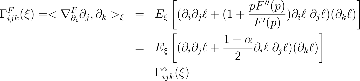
Amari’s α−geometry is a special case of the F−geometry.

Proof

Let F(p) = L_α(p), L_α(p) is the α−embedding of Amari.

The components ${\mathrm{\Gamma }}_{ijk}^{\alpha }$ of the α−connection are given by

(27)

From Equation (26), when F (p) = L_α(p)

we have

$$F^{\prime }(p)={L^{\prime }}_{\alpha }(p)=p^{-\left(\frac{1+\alpha }{2}\right)}$$

(28)

$$F^{″}(p)={L^{″}}_{\alpha }(p)=-\frac{1+\alpha }{2}{p}^{-\left(\frac{3+\alpha }{2}\right)}.$$

(29)

Then we get

$$1+\frac{p{F}^{″}(p)}{F^{\prime }(p)}=1+\frac{p{L^{″}}_{\alpha }(p)}{{L^{\prime }}_{\alpha }(p)}=\frac{1-\alpha }{2}$$

(30)

Hence

(31)

which are the components of the α−connection. Hence F−connection reduces to α−connection. Thus we obtain that α−geometry is a special case of F−geometry. □

Remark 2.6

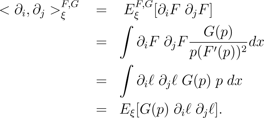
Burbea [14] introduced the concept of weighted Fisher information metric using a positive continuous function. We use this idea to define weighted F−metric and weighted F−connections. Let G: (0, ∞) → ℝ be a positive smooth function and F be an embedding, define (F, G)−expectation of a random variable with respect to the distribution p_ξ as

$$E_{\xi }^{F,G}(f)=\int f(x)\frac{G(p)}{p{(F^{\prime }(p))}^2}dx.$$

(32)

Define (F, G)−metric$<,{>}_{\xi }^{F,G}$ in$T_{p_{\xi }}(S)$ by

(33)

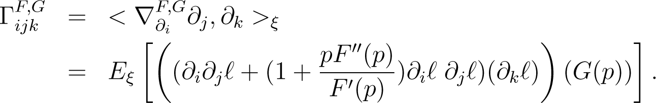
Define (F, G)−connection as

(34)

When G(p) = 1, (F, G)−connection reduces to the F−connection and the metric <, >^F,G reduces to the Fisher information metric. This is a more general way of defining Riemannian metrics and affine connections on a statistical manifold.

3. Dual Affine Connections

Definition 3.1

Let M be a Riemannian manifold with a Riemannian metric g. Two affine connections, ∇ and ∇^∗ on the tangent bundle are said to be dual connections with respect to the metric g if

$$Zg(X,Y)=g({\nabla }_{Z}X,Y)+g(X,{\nabla }_Z^{*}Y)$$

(35)

holds for any vector fields X, Y, Z on M.

Theorem 3.2

Let F, H be two embeddings of statistical manifold S into the space ℝ_X of random variables. Let G be a positive smooth function on (0, ∞). Then the (F, G)−connection ∇^F,G and the (H, G)−connection ∇^H,G are dual connections with respect to the (F, G)−metric iff the functions F and H satisfy

$$H^{\prime }(p)=\frac{G(p)}{p{F}^{\prime }(p)}$$

(36)

We call such an embedding H as a G−dual embedding of F.

The components of the dual connection ∇^H,G can be written as

$${\mathrm{\Gamma }}_{ijk}^{H,G}={\displaystyle \int \left({\partial }_i{\partial }_j\ell +(\frac{p{G}^{\prime }(p)}{G(p)}-\frac{p{F}^{″}(p)}{F^{\prime }(p)}){\partial }_i\ell {\partial }_j\ell \right){\partial }_k\ell G(p)pdx}.$$

(37)

Proof

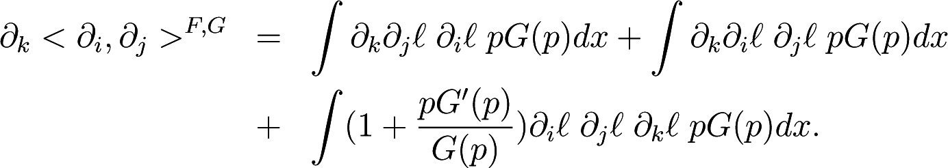
∇^F,G and ∇^H,G are dual connections with respect to the G−metric means,

$${\partial }_k<{\partial }_i,{\partial }_j{>}^{F,G}=<{\nabla }_{{\partial }_k}^{F,G}{\partial }_i,{\partial }_j{>}^{F,G}+<{\partial }_i,{\nabla }_{{\partial }_k}^{H,G}{\partial }_j{>}^{F,G}.$$

(38)

for any basis vectors ∂_i, ∂_j, ∂_k ∈ T_ξ(S).

(39)

(40)

Then the condition (38) holds iff

$$\begin{array}{r}{\displaystyle \int [2+\frac{p{F}^{″}(p)}{F^{\prime }(p)}+\frac{p{H}^{″}(p)}{H^{\prime }(p)}]{\partial }_i\ell {\partial }_j\ell {\partial }_k\ell pG(p)dx}=\\ {\displaystyle \int [1+\frac{p{G}^{\prime }(p)}{G(p)}]{\partial }_i\ell {\partial }_j\ell {\partial }_k\ell pG(p)dx}\end{array}$$

(41)

$$\iff [2+\frac{p{F}^{″}(p)}{F^{\prime }(p)}+\frac{p{H}^{″}(p)}{H^{\prime }(p)}]=1+\frac{p{G}^{\prime }(p)}{G(p)}.$$

(42)

$$\iff 1+\frac{p{H}^{″}(p)}{H^{\prime }(p)}=\frac{p{G}^{\prime }(p)}{G(p)}-\frac{p{F}^{″}(p)}{F^{\prime }(p)}$$

(43)

$$\iff \frac{H^{″}(p)}{H^{\prime }(p)}=\frac{G^{\prime }(p)}{G(p)}-\frac{F^{″}(p)}{F^{\prime }(p)}-\frac{1}{p}\iff H^{\prime }(p)=\frac{G(p)}{p{F}^{\prime }(p)}.$$

(44)

Hence ∇^F,G and ∇^H,G are dual connections with respect to the (F, G)−metric iff Equation (36) holds. From Equation (43), we can rewrite the components of dual connection ∇^H,G as

$${\mathrm{\Gamma }}_{ijk}^{H,G}={\displaystyle \int \left({\partial }_i{\partial }_j\ell +(\frac{p{G}^{\prime }(p)}{G(p)}-\frac{p{F}^{″}(p)}{F^{\prime }(p)}){\partial }_i\ell {\partial }_j\ell \right)}{\partial }_k\ell G(p)pdx.$$

(45)

Corollary 3.3

Amari’s 0−connection is the only self dual F−connection with respect to the Fisher information metric.

Proof

From Theorem 3.2, for G(p) = 1 the F−connection ∇^F and the H−connection ∇^H are dual connections with respect to the Fisher information metric iff the functions F and H satisfy

$$H^{\prime }(p)=\frac{1}{p{F}^{\prime }(p)}$$

(46)

Thus the F−connection ∇^F is self dual iff the embedding F satisfies the condition

$$F^{\prime }(p)=\frac{1}{p{F}^{\prime }(p)}\iff F^{\prime }(p)=p^{-(\frac{1}{2})}\iff F(p)=2p^{\frac{1}{2}}=L_0(p).$$

(47)

That is, Amari’s 0–connection is the only self dual F–connection with respect to the Fisher information metric.

So far, we have considered the statistical manifold S as a subset of P(X), the set of all probability measures on X. Now we relax the condition ∫p(x)dx = 1, and consider S as a subset of $\tilde{P}(X)$, which is defined by

$$\tilde{P}(X):=\{p:X\to ℝ/p(x)>0(\forall x\in X);{\displaystyle \underset{X}{\int }p(x)dx<\infty \}.}$$

(48)

Definition 3.4

Let M be a Riemannian manifold with a Riemannian metric g. Let ∇ be an affine connection on M. If there exists a coordinate system [θⁱ] of M such that ∇_∂i∂_j = 0 then we say that ∇ is flat, or alternatively M is flat with respect to ∇, and we call such a coordinate system [θⁱ] an affine coordinate system for ∇.

Definition 3.5

Let S = {p(x; ξ) / ξ = [ξ¹, …, ξⁿ] ∈ $\mathbb{E}$ ⊆ ℝⁿ} be an n−dimensional statistical manifold. If for some coordinate system [θⁱ]; i = 1, …, n

$${\partial }_i{\partial }_{j}F(p(x;\theta ))=0$$

(49)

then we can see from Equation (19) that [θⁱ] is an F−affine coordinate system and that S = {p_θ} is F−flat. We call such S as an F−affine manifold.

The condition (49) is equivalent to the existence of the functions C, F₁, …, F_n on X such that

$$F(p(x;\theta ))=C(x)+{\displaystyle \sum _{i=1}^n{\theta }^i{F}_i(x)}$$

(50)

Theorem 3.6

For any embedding F, $\tilde{P}(X)$ is an F−affine manifold for finite X.

Proof

Let X = {x₁, …., x_n} be a finite set constituted by n elements. Let F_i: X→ ℝ be the functions defined by F_i(x_j) = δ_ij for i, j = 1, …, n. Let us define n coordinates [θⁱ] by

$${\theta }^i=F(p(x_i))$$

(51)

Then we get $F(p(x))={\displaystyle {\sum }_{i=1}^n{\theta }^i{F}_i(x)}$. Therefore $\tilde{P}(X)$ is an F–affine manifold for any embedding F(p).

Remark 3.7

Zhang [13] introduced ρ-representation, which is a generalization of α-representation of Amari. Zhang’s geometry is defined using this ρ-representation together with a convex function. Zhang also defined the ρ-affine family of density functions and discussed its dually flat structure. The F−geometry defined using a general F-representation is different from the Zhang’s geometry. The metric defined in the F-embedding approach is the Fisher information metric and the Riemannian metric defined using the ρ-representation is different from the Fisher information metric. The F-connections defined are not in general dually flat and are different from the dual connections defined by Zhang.

Remark 3.8

On a statistical manifold S, we introduced a dualistic structure (g, ∇^F, ∇^H), where g is the Fisher information metric and ∇^F, ∇^H are the dual connections with respect to the Fisher information metric. Since F-connections are symmetric, the manifold S is flat with respect to ∇^F iff S is flat with respect to ∇^H. Thus if S is flat with respect to ∇^F, then (S, g, ∇^F, ∇^H) is a dually flat space. The dually flat spaces are important in statistical estimation [4].

4. Invariance of the Geometric Structures

For the statistical manifold S = {p(x; ξ) | ξ ∈ $\mathbb{E}$ ⊆ ℝⁿ}, the parameters are merely labels attached to each point p ∈ S, hence the intrinsic geometric properties should be independent of these labels. Consequently, it is natural to consider the invariance properties of the geometric structures under suitable transformations of the variables in a statistical manifold. Here we can consider two kinds of invariance of the geometric structures; covariance under re-parametrization of the parameter of the manifold and invariance under the transformations of the random variable [15]. Now let us investigate the invariance properties of the F-geometric structures defined in Section 2.

4.1. Covariance under Re-Parametrization

Let [θⁱ] and [η_j] be two coordinate systems on S, which are related by an invertible transformation η = η(θ). Let us denote ${\partial }_i=\frac{\partial }{\partial {\theta }^i}$ and ${\partial }^j=\frac{\partial }{\partial {\eta }_j}$. Let the coordinate expressions of the metric g be given by g_ij =<∂_i, ∂_j> and ${\tilde{g}}_{ij}=<{\partial }^i,{\partial }^j>$. Let the components of the connection ∇ with respect to the coordinates [θⁱ] and [η_j] be given by Γ_ijk, ${\tilde{\mathrm{\Gamma }}}_{ijk}$ respectively.

Then the covariance of the metric g and the connection ∇ under the re-parametrization means,

$${\tilde{g}}_{ij}={\displaystyle \sum _m{\displaystyle \sum _n\frac{\partial {\theta }^m}{\partial {\eta }_i}\frac{\partial {\theta }^n}{\partial {\eta }_j}{g}_{mn}}}$$

(52)

$${\tilde{\mathrm{\Gamma }}}_{ijk}={\displaystyle \sum _{m,n,h}\frac{\partial {\theta }^m}{\partial {\eta }_i}\frac{\partial {\theta }^n}{\partial {\eta }_j}\frac{\partial {\theta }^h}{\partial {\eta }_k}{\mathrm{\Gamma }}_{mnh}+{\displaystyle \sum _{m,h}\frac{\partial {\theta }^h}{\partial {\eta }_k}\frac{{\partial }^2{\theta }^m}{\partial {\eta }_i\partial {\eta }_j}{g}_{mh}}}$$

(53)

Lemma 4.1

The Fisher information metric g is covariant under re-parametrization.

Proof

The components of the Fisher information metric with respect to the coordinate system [θⁱ] are given by

$$g_{ij}(\theta )=<{\partial }_i,{\partial }_j{>}_{\theta }={\displaystyle \int {\partial }_{i}p(x;\theta ){\partial }_{j}p(x;\theta )\frac{1}{p(x;\theta )}dx.}$$

(54)

Let $\tilde{p}(x;\eta )=p(x;\theta (\eta ))$. then the components of the Fisher information metric with respect to the coordinate system [η_j] are given by

$${\tilde{g}}_{ij}(\eta )=<{\partial }^i,{\partial }^j{>}_{\eta }={\displaystyle \int {\partial }^i\tilde{p}(x;\eta ){\partial }^j\tilde{p}(x;\eta )\frac{1}{\tilde{p}(x;\eta )}dx.}$$

(55)

Since

$${\partial }^i\tilde{p}(x;\eta )={\displaystyle \sum _m\frac{\partial {\theta }^m}{\partial {\eta }_i}\frac{\partial p(x;\theta (\eta ))}{\partial {\theta }^m}}$$

(56)

we can write

(57)

Lemma 4.2

The F−connection ∇^F is covariant under re-parametrization.

Proof

Let the components of ∇^F with respect to the coordinates [θⁱ] and [η_j] be given by Γ_ijk, ${\tilde{\mathrm{\Gamma }}}_{ijk}$ respectively.

Let $\tilde{p}(x;\eta )=p(x;\theta (n))$. Let us denote log p(x; θ) by ℓ(x; θ) and $\log \tilde{p}(x;\eta )$ by $\tilde{\ell }(x;\eta )$.

The components of the F−connection ∇^F with respect to the coordinate system [θⁱ] are given by

$${\mathrm{\Gamma }}_{ijk}={\displaystyle \int \left({\partial }_i{\partial }_j\ell (x;\theta )+(1+\frac{p{F}^{″}(p)}{F^{\prime }(p)}){\partial }_i\ell (x;\theta ){\partial }_j\ell (x;\theta )\right){\partial }_k\ell (x;\theta )p(x;\theta )dx}$$

(58)

The components of ∇^F with respect to the coordinate system [η_j] are given by

$${\tilde{\mathrm{\Gamma }}}_{ijk}={\displaystyle \int \left({\partial }^i{\partial }^j\tilde{\ell }(x;\eta )+(1+\frac{\tilde{p}{F}^{″}(\tilde{p})}{F^{\prime }(\tilde{p})}){\partial }^i\tilde{\ell }(x;\eta ){\partial }^j\tilde{\ell }(x;\eta )\right){\partial }^k\tilde{\ell }(x;\eta )\tilde{p}(x;\eta )dx}$$

(59)

We can write

$${\partial }^i\tilde{\ell }(x;\eta )={\displaystyle \sum _m\frac{\partial {\theta }^m}{\partial {\eta }_i}\frac{\partial \ell (x;\theta (\eta ))}{\partial {\theta }^m}}$$

(60)

Then

$${\partial }^i{\partial }^j\tilde{\ell }(x;\eta )={\displaystyle \sum _{m,n}\frac{\partial {\theta }^m}{\partial {\eta }_i}\frac{\partial {\theta }^n}{\partial {\eta }_j}\frac{{\partial }^2\ell (x;\theta (\eta ))}{\partial {\theta }^m\partial {\theta }^n}+{\displaystyle \sum _m\frac{{\partial }^2{\theta }^m}{\partial {\eta }_i\partial {\eta }_j}\frac{\partial \ell (x;\theta (\eta ))}{\partial {\theta }^m}}}$$

(61)

$${\partial }^i\tilde{\ell }(x;\eta ){\partial }^j\tilde{\ell }(x;\eta )={\displaystyle \sum _{m,n}\frac{\partial {\theta }^m}{\partial {\eta }_i}\frac{\partial {\theta }^n}{\partial {\eta }_j}\frac{\partial \ell (x;\theta (\eta ))}{\partial {\theta }^m}}\frac{\partial \ell (x;\theta (\eta ))}{\partial {\theta }^n}$$

(62)

$${\partial }^k\tilde{\ell }(x;\eta )={\displaystyle \sum _h\frac{\partial {\theta }^h}{\partial {\eta }_k}\frac{\partial \ell (x;\theta (\eta ))}{\partial {\theta }^h}}$$

(63)

Hence we get

(64)

Hence we showed that F−connections are covariant under re-parametrization of the parameter. The covariance under re-parametrization actually means that the metric and connections are coordinate independent. Hence we obtained that the F−geometry is coordinate independent.

4.2. Invariance Under the Transformation of the Random Variable

Amari and Nagaoka [4] defined the invariance of Riemannian metric and connections on a statistical manifold under a transformation of the random variable as follows,

Definition 4.3

Let S = {p(x; ξ) | ξ ∈ $\mathbb{E}$ ⊆ ℝⁿ} be a statistical manifold defined on a sample space X. Let x, y be random variables defined on sample spaces X, Y respectively and φ be a transformation of x to y. Assume that this transformation induces a model S′ = {q(y; ξ) | ξ ∈ $\mathbb{E}$ ⊆ ℝⁿ} on Y.

Let λ: S → S′ be a diffeomorphism defined as

$$\lambda (p_{\xi })=q_{\xi }$$

(65)

Let g =<>, g′ =<>′ be two Riemannian metrics defined on S and S′ respectively. Let ∇, ∇′ be two affine connections on S and S′ respectively. Then the invariance properties are given by

$$<X,Y{>}_p=<{\lambda }_{*}(X),{\lambda }_{*}(Y){{>}^{\prime }}_{\lambda (p)}\forall X,Y\in T_p(S)$$

(66)

$${\lambda }_{*}({\nabla }_{X}Y)={{\nabla }^{\prime }}_{{\lambda }_{*}(X)}{\lambda }_{*}(Y)$$

(67)

where λ_∗ is the push forward map associated with the map λ, which is defined by

$${\lambda }_{*}{(X)}_{\lambda (p)}={(d\lambda )}_p(X)$$

(68)

Now we discuss the invariance properties of the F−geometry under suitable transformations of the random variable. Let us restrict ourselves to the case of smooth one-to-one transformations of the random variable that are in fact statistically interesting. Amari and Nagaoka [4] mentioned a transformation, the sufficient statistic of the parameter of the statistical model, which is widely used in statistical estimation. In fact the one-to-one transformations of the random variable are trivial examples of sufficient statistic.

Consider a statistical manifold S = {p(x; ξ) | ξ ∈ $\mathbb{E}$ ⊆ ℝⁿ} defined on a sample space X. Let ϕ be a smooth one-to-one transformation of the random variable x to y. Then the density function q(y; ξ) of the induced model S′ takes the form

$$q(y:\xi )=p(w(y);\xi )w^{\prime }(y)$$

(69)

where w is a function such that x = w(y) and ${\varphi }^{\prime }(x)=\frac{1}{w^{\prime }(\varphi (x))}$.

Let us denote log q(y; ξ) by ℓ(q_y) and log p(x; ξ) by ℓ(p_x).

Lemma 4.4

The Fisher information metric and Amari’s α-connections are invariant under smooth one-to-one transformations of the random variable.

Proof

Let ϕ be a smooth one-to-one transformation of the random variable x to y. From Equation (69)

$$p(x;\xi )=q(\varphi (x);\xi ){\varphi }^{\prime }(x)$$

(70)

$${\partial }_i\ell (q_y)={\partial }_i\ell (p_{w(y)})$$

(71)

$${\partial }_i\ell (q_{\varphi (x)})={\partial }_i\ell (p_x)$$

(72)

The Fisher information metric g′ on the induced manifold S′ is given by

(73)

which is the Fisher information metric on S.

The components of Amari’s α−connections on the induced manifold S′ are given by

(74)

which are the components of Amari’s α−connections on the manifold S. Thus we obtained that the Fisher information metric and Amari’s α-connections are invariant under smooth one-to-one transformations of the random variable.

Now we prove that α-connections are the only F−connections that are invariant under smooth one-to-one transformations of the random variable.

Theorem 4.5

Amari’s α-connections are the only F−connections that are invariant under smooth one-to-one transformations of the random variable.

Proof

Let ϕ be a smooth one-to-one transformation of the random variable x to y. The components of the F −connection of the induced manifold S′ are

(75)

and the components of the F−connection of the manifold S are

(76)

Then by equating the components ${{\mathrm{\Gamma }}^{\prime }}_{ijk}^F(q_{\xi }),{\mathrm{\Gamma }}_{ijk}^F(p_{\xi })$ of the F–connection, we get

(77)

Then it follows that the condition for F–connection to be invariant under the transformation ϕ is given by

$$\frac{p{F}^{″}(p)}{F^{\prime }(p)}=k,$$

(78)

where k is a real constant.

Hence it follows from the Euler’s homogeneous function theorem that the function F′ is a positive homogeneous function in p of degree k. So

$$F^{\prime }(\lambda p)={\lambda }^k{F}^{\prime }(p)\text{for}\lambda >0.$$

(79)

Since F′ is a positive homogeneous function in the single variable p, without loss of generality we can take,

$$F^{\prime }(p)=p^k.$$

(80)

Therefore

$$F(p)=\{\begin{array}{cc}\frac{p^{k+1}}{k+1}& k\ne -1\\ \log p& k=-1\end{array}$$

(81)

Let

$$k=\frac{-(1+\alpha )}{2},\alpha \in ℝ.$$

(82)

we get

$$F(p)=\{\begin{array}{cc}\frac{2}{1-\alpha }{p}^{\frac{1-\alpha }{2}}& \alpha \ne -1\\ \log p& \alpha =-1\end{array}$$

(83)

which is nothing but Amari’s α–embeddings L_α(p). Hence we obtain that Amari’s α–connections are the only F–connections that are invariant under smooth one-to-one transformations of the random variable.

Remark 4.6

In Section 2, we defined (F, G)-connections using a general embedding function F and a positive smooth function G. We can show that (F, G)-connection is invariant under smooth one-to-one transformation of the random variable when G(p) = c, where c is a real constant and F (p) = L_α(p) (proof is similar to that of Theorem 4.5). The notion of (F, G)−metric and (F, G)−connection provides a more general way of introducing geometric structures on a manifold. We were able to show that the Fisher information metric (up to a constant) and Amari’s α−connections are the only metric and connections belonging to this class that are invariant under both the transformation of the parameter and the one-to-one transformation of the random variable.

5. Conclusions

The Fisher information metric and Amari’s α−connections are widely used in the theory of information geometry and have an important role in the theory of statistical estimation. Amari’s α−connections are defined using a one parameter family of functions, the α−embeddings. We generalized this idea to introduce geometric structures on a statistical manifold S. We considered a general embedding function F of S into ℝ_X and obtained a geometric structure on S called the F−geometry. Amari’s α−geometry is a special case of F −geometry. A more general way of defining Riemannian metrics and affine connections on a statistical manifold S is given using a positive continuous function G and the embedding F.

Amari’s α−geometry is the only F−geometry that is invariant under both the transformation of the parameter and the random variable or equivalently under the sufficient statistic. We can relax the condition of invariance under the sufficient statistic and can consider other statistically significant transformations as well, which then gives an F−geometry other than α−geometry that is invariant under these statistically significant transformations. We believe that the idea of F −geometry can be used in the further development of the geometric theory of q-exponential families. We look forward to studying these problems in detail later.

References

- Amari, S. Differential geometry of curved exponential families-curvature and information loss. Ann. Statist 1982, 10, 357–385. [Google Scholar]
- Amari, S. Differential-Geometrical Methods in Statistics; Lecture Notes in Statistics; Volume 28, Springer-Verlag: New York, NY, USA, 1985. [Google Scholar]
- Amari, S.; Kumon, M. Differential geometry of Edgeworth expansions in curved exponential family. Ann. Inst. Statist. Math 1983, 35, 1–24. [Google Scholar]
- Amari, S.; Nagaoka, H. Methods of Information Geometry, Translations of Mathematical Monographs; Oxford University Press: Oxford, UK, 2000. [Google Scholar]
- Barndorff-Nielsen, O.E.; Cox, D.R.; Reid, N. The role of differential geometry in statistical theory. Internat. Statist. Rev 1986, 54, 83–96. [Google Scholar]
- Dawid, A.P. A Discussion to Efron’s paper. Ann. Statist 1975, 3, 1231–1234. [Google Scholar]
- Efron, B. Defining the curvature of a statistical problem (with applications to second order efficiency). Ann. Statist 1975, 3, 1189–1242. [Google Scholar]
- Efron, B. The geometry of exponential families. Ann. Statist 1978, 6, 362–376. [Google Scholar]
- Murray, M.K.; Rice, R.W. Differential Geometry and Statistics; Chapman & Hall: London, UK, 1995. [Google Scholar]
- Rao, C.R. Information and accuracy attainable in the estimation of statistical parameters. Bull. Calcutta. Math. Soc 1945, 37, 81–91. [Google Scholar]
- Chentsov, N.N. Statistical Decision Rules and Optimal Inference; Transted in English; Translation of the Mathematical Monographs; American Mathematical Society: Providence, RI, USA, 1982. [Google Scholar]
- Corcuera, J.M.; Giummole, F. A characterization of monotone and regular divergences. Ann. Inst. Statist. Math 1998, 50, 433–450. [Google Scholar]
- Zhang, J. Divergence function, duality and convex analysis. Neur. Comput 2004, 16, 159–195. [Google Scholar]
- Burbea, J. Informative geometry of probability spaces. Expo Math 1986, 4, 347–378. [Google Scholar]
- Wagenaar, D.A. Information Geometry for Neural Networks, Available online: http://www.danielwagenaar.net/res/papers/98-Wage2.pdf (accessed on 13 December 2013).
- Amari, S.; Ohara, A.; Matsuzoe, H. Geometry of deformed exponential families: Invariant, dually flat and conformal geometries. Physica A 2012, 391, 4308–4319. [Google Scholar]
© 2014 by the authors; licensee MDPI, Basel, Switzerland This article is an open access article distributed under the terms and conditions of the Creative Commons Attribution license (http://creativecommons.org/licenses/by/3.0/).
Share and Cite
V., H.K.; S., S.M.K. F-Geometry and Amari’s α-Geometry on a Statistical Manifold. Entropy 2014, 16, 2472-2487. https://0-doi-org.brum.beds.ac.uk/10.3390/e16052472
V. HK, S. SMK. F-Geometry and Amari’s α-Geometry on a Statistical Manifold. Entropy. 2014; 16(5):2472-2487. https://0-doi-org.brum.beds.ac.uk/10.3390/e16052472
Chicago/Turabian StyleV., Harsha K., and Subrahamanian Moosath K. S. 2014. "F-Geometry and Amari’s α-Geometry on a Statistical Manifold" Entropy 16, no. 5: 2472-2487. https://0-doi-org.brum.beds.ac.uk/10.3390/e16052472