Black-Box Optimization Using Geodesics in Statistical Manifolds †

Laboratoire de Recherche en Informatique, Université Paris-Sud, 91400 Orsay, France
†
This paper is an extended version of our paper published in 34th International Workshop on Bayesian Inference and Maximum Entropy Methods in Science and Engineering, 21–26 September 2014, Château Clos Lucé, Parc Leonardo Da Vinci, Amboise, France.
Entropy 2015, 17(1), 304-345; https://0-doi-org.brum.beds.ac.uk/10.3390/e17010304
Submission received: 8 October 2014
/
Accepted: 7 January 2015
/
Published: 13 January 2015
(This article belongs to the Special Issue Information, Entropy and Their Geometric Structures)
Abstract
:Information geometric optimization (IGO) is a general framework for stochastic optimization problems aiming at limiting the influence of arbitrary parametrization choices: the initial problem is transformed into the optimization of a smooth function on a Riemannian manifold, defining a parametrization-invariant first order differential equation and, thus, yielding an approximately parametrization-invariant algorithm (up to second order in the step size). We define the geodesic IGO update, a fully parametrization-invariant algorithm using the Riemannian structure, and we compute it for the manifold of Gaussians, thanks to Noether’s theorem. However, in similar algorithms, such as CMA-ES (Covariance Matrix Adaptation - Evolution Strategy) and xNES (exponential Natural Evolution Strategy), the time steps for the mean and the covariance are decoupled. We suggest two ways of doing so: twisted geodesic IGO (GIGO) and blockwise GIGO. Finally, we show that while the xNES algorithm is not GIGO, it is an instance of blockwise GIGO applied to the mean and covariance matrix separately. Therefore, xNES has an almost parametrization-invariant description.
Keywords:
black-box; optimization; geodesics; Gaussian; information geometry; natural gradient; Noether; learning rate; IGO; xNES1. Introduction
Consider an objective function f: X → ℝ to be minimized. We suppose we have absolutely no knowledge about f: the only thing we can do is ask for its value at any point x ∈ X (black-box optimization) and that the evaluation of f is a costly operation. We are going to study algorithms that can be described in the IGO framework (see [1]).
We consider the following optimization procedure:
We choose (Pθ)θ∈Θ a family of probability distributions (which will be given a Riemannian manifold structure, following [2]) on X and an initial probability distribution
. Now, we replace f by F: Θ → ℝ (for example
), and we optimize F by gradient descent, corresponding to the gradient flow:
However, because of the gradient, this equation depends entirely on the parametrization we chose for Θ, which is disturbing: we do not want to have two different updates, because we chose different parameters to represent the objects with which we are working. Moreover, in the case of a function with several local minima, changing the parametrization can change the attained optimum (see [3], for example). That is why invariance is a design principle behind IGO. More precisely, we want invariance with respect to monotone transformations of f and invariance under reparametrization of Θ.
The IGO framework uses the geometry of the family Θ, which is given by the Fisher metric to provide a differential equation on θ with the desired properties, but because of the discretization of time needed to obtain an explicit algorithm, we lose invariance under reparametrization of θ: two IGO algorithms applied to the same function to be optimized, but with different parametrizations, coincide only at first order in the step size. A possible solution to this problem is geodesic IGO (GIGO), introduced here (see also IGO-Maximum Likelihoodin [1], for example.): the initial direction of the update at each step of the algorithm remains the same as in IGO, but instead of moving straight for the chosen parametrization, we use the Riemannian manifold structure of our family of probability distributions (see [2]) by following its geodesics.
Finding the geodesics of a Riemannian manifold is not always easy, but Noether’s theorem will allow us to obtain quantities that are preserved along the geodesics, thus allowing, in the case of Gaussian distributions, one to obtain a first order differential equation satisfied by the geodesics, which makes their computation easier.
Although the geodesic IGO algorithm is not, strictly speaking, parametrization-invariant when no closed form for the geodesics is known, it is possible to compute them at arbitrary precision without increasing the numbers of objective function calls.
The first two sections are preliminaries: in Section 2, we recall the IGO algorithm, introduced in [1], and in Section 3, after a reminder about Riemannian geometry, we state Noether’s theorem, which will be our main tool to compute the GIGO update for Gaussian distributions.
In Section 4, we consider Gaussian distributions with a covariance matrix proportional to the identity matrix: this space is isometric to the hyperbolic space, and the geodesics of the latter are known.
In Section 5.1, we consider the general Gaussian case, and we use Noether’s theorem to obtain two different sets of equations to compute the GIGO update. The equations are known (see [4–6]), but the connection with Noether’s theorem has not been mentioned. We then give the explicit solution for these equations, from [5].
In Section 6, we recall quickly the xNES and CMA-ESupdates, and we introduce a slight modification of the IGO algorithm to incorporate the direction-dependent learning rates used in CMA-ESand xNES. We then compare these different algorithms and prove that xNES is not GIGO in general, and we finally introduce a new family of algorithms extending GIGO and recovering xNES from abstract principles.
Finally, Section 7 presents numerical experiments, which suggest that when using GIGO with Gaussian distributions, the step size must be chosen carefully.
2. Definitions: IGO, GIGO
In this section, we recall what the IGO framework is and we define the geodesic IGO update. Consider again Equation (1):
As we saw in the Introduction:
- The gradient depends on the parametrization of our space of probability distributions (see Section 2.3 for an example).
- The equation is not invariant under monotone transformations of f. For example, the optimization for 10f moves ten times faster than the optimization for f.
In this section, we recall how IGO deals with this (see [1] for a better presentation).
2.1. Invariance under Reparametrization of θ: Fisher Metric
In order to achieve invariance under reparametrization of θ, it is possible to turn our family of probability distributions into a Riemannian manifold (this is the main topic of information geometry; see [2]), which allows us to use a canonical, parametrization-invariant gradient (called the natural gradient).
Definition 1. Let P, Q be two probability distributions on X. The Kullback–Leibler divergence of Q from P is defined by:
By definition, it does not depend on the parametrization. It is not symmetrical, but if for all x, the application θ ⟼ Pθ(x) is C2, then a second-order expansion yields:
where:
This is enough to endow the family (Pθ)θ∈Θ with a Riemannian manifold structure: a Riemannian manifold M is a differentiable manifold, which can be seen as pieces of ℝn glued together, with a metric. The metric at x is a symmetric positive-definite quadratic form on the tangent space of M at x: it indicates how expensive it is to move in a given direction on the manifold. We will think of the updates of the algorithms that we will be studying as paths on M.
The matrix I(θ) is called the “Fisher information matrix”, and the metric it defines is called the “Fisher metric”.
Given a metric, it is possible to define a gradient attached to this metric; the key property of the gradient is that for any smooth function f:
where
is the dot product in metric I. Therefore, in order to keep the property of Equation (5), we must have
.
We have therefore the following gradient (called the “natural gradient”; see [2]):
and since the Kullback–Leibler divergence does not depend on the parametrization, neither does the natural gradient.
Later in this paper, we will study families of Gaussian distributions. The following proposition gives the Fisher metric for these families.
Proposition 1. Let (Pθ)θ∈Θ be a family of normal probability distributions: If μ and Σ are C1, the Fisher metric is given by:
As we will often be working with Gaussian distributions, we introduce the following notation:
Notation 1.
is the manifold of Gaussian distributions in dimension d, equipped with the Fisher metric. is the manifold of Gaussian distributions in dimension d, with the covariance matrix proportional to identity in the canonical basis of ℝd, equipped with the Fisher metric.
2.2. IGO Flow, IGO Algorithm
In IGO [1], invariance with respect to monotone transformations is achieved by replacing f by the following transform; we set:
a non-increasing function w: [0; 1] → ℝ is chosen (the selection scheme), and finally,
(this definition has to be slightly changed if the probability of a tie is not zero, see [1] for more details). By performing a gradient descent on
, we obtain the “IGO flow”:
Notice that the function we are optimizing is
and not
(the second function is constant and always equal to
). In particular, the function for which we are performing the gradient descent changes at each step, although their optimum (a Dirac at the minimum of f) does not: the IGO flow is not a gradient flow; it is simply a vector flow given by the gradient of interrelated functions.
For practical implementation, the integral in (9) has to be approximated. For the integral itself, the Monte-Carlo method is used; N values (x1, …, xN) are sampled from the distribution
, and the integral becomes:
and we approximate
by
, where rk(xi) = |{j, f(xj) < f(xi)}|: it can be proven (see [1]) that
(here again, we are assuming that there are no ties).
We now have an algorithm that can be used in practice if the Fisher information matrix is known.
Definition 1. The IGO update associated with parametrization θ, sample size N, step size δt and selection scheme w is given by the following update rule:
We call IGO speed the vector
Notice that one could start directly with the
rather than w, as we will do later.
Replacing f by its expected value under a probability distribution Pθ and optimizing over θ using the natural gradient have already been discussed. For example, in the case of a function f defined on {0, 1}n, IGO with the Bernoulli distributions yields the algorithm, PBIL[9]. Another similar approach (stochastic relaxation) is given in [10]. For a continuous function, as we will see later, the IGO framework recovers several known ranked-based natural gradient algorithms, such as pure rank-μ CMA-ES [11], xNES or SNES (Separable Natural Evolution Strategies) [12]. See [13] or [14] for other, not necessarily gradient-based, optimization algorithms on manifolds.
2.3. Geodesic IGO
Although the IGO flow associated with a family of probability distributions is intrinsic (it only depends on the family itself, not the parametrization we choose for it), the IGO update is not. However, the difference between two steps of IGO that differ only by the parametrization is only O(δt2), whereas the different between two vanilla gradient descents with different parametrizations is O(δt).
Intuitively, the reason for this difference is that two IGO algorithms start at the same point and follow “straight lines” with the same initial speed, but the definition of “straight lines” changes with the parametrization.
For instance, in the case of Gaussian distributions, let us consider two different IGO updates with Gaussian distributions in dimension one, the first one with parametrization (μ, σ) and the second one with parametrization (μ, c := σ2). We suppose that the IGO speed for the first algorithm is
. The corresponding IGO speed in the second parametrization is given by the identity
. Therefore, the first algorithm gives the standard deviation
and the variance
.
The geodesics of a Riemannian manifold are the generalization of the notion of a straight line: they are curves that locally minimize length. In particular, given two points a and b on the Riemannian manifold M, the shortest path from a to b is always a geodesic (the converse is not true, though). The notion will be explained precisely in Section 3, but let us define the geodesic IGO algorithm, which follows the geodesics of the manifold instead of following the straight lines for an arbitrary parametrization.
Definition 2 (GIGO). The geodesic IGO update (GIGO) associated with sample size N, step size δt and selection scheme w is given by the following update rule:
where:
is the IGO speed and is the exponential of the Riemannian manifold Θ. Namely,
is the endpoint of the geodesic of Θ starting at θt, with initial speed Y, after a time δt. By definition, this update does not depend on the parametrization θ.
Notice that while the GIGO update is compatible with the IGO flow (in the sense that when δt → 0 and N → ∞, a parameter θt updated according to the GIGO algorithm is a solution of Equation (9), the equation defining the IGO flow), it not necessarily an IGO update. More precisely, the GIGO update is an IGO update if and only if the geodesics of Θ are straight lines for some parametrization (by Beltrami’s theorem, this is equivalent to Θ having constant curvature).
This is a particular case of a retraction [14]: a map from the tangent bundle of a manifold to the manifold itself satisfying a rigidity condition. Arguably, the Riemannian exponential is the most natural retraction, since it depends only on the Riemannian manifold itself and not on any decomposition. However, in general, the geodesics are difficult to compute.
In the next section, we will state Noether’s theorem, which will be our main tool to compute the GIGO update for Gaussian distributions.
3. Riemannian Geometry, Noether’s Theorem
3.1. Riemannian Geometry
The goal of this section is to state Noether’s theorem. See [15] for the proofs and [16] or [17] for a more detailed presentation. Noether’s theorem states that if a system has symmetries, then there are invariants attached to these symmetries. Firstly, we need some definitions.
Definition 3 (Motion in a Lagrangian system). Let M be a differentiable manifold, TM the set of tangent vectors on M (a tangent vector is identified by the point at which it is tangent and a vector in the tangent space) and differentiable function called the Lagrangian function (in general, it could depend on t). A “motion in the Lagrangian system (M, ) from x to y” is map γ : [t0, t1] → M, such that:
- γ(t0) = x
- γ(t1) = y
- γ is a local extremum of the functional:among all curves c: [t0, t1] → M, such that c(t0) = x, and c(t1) = y.
For example, when (M, g) is a Riemannian manifold, the length of a curve γ between γ(t0) and γ(t1) is:
The curves that follow the shortest path between two points x, y ∈ M are therefore the minima γ of the functional (15), such that γ(t0) = x and γ(t1) = y, and the corresponding Lagrangian function is
. However, any curve following the shortest trajectory will have minimum length. For example, if γ1: [a, b] → M is a curve of the shortest path, so is γ2: t ↦ γ1(t2): these two curves define the same trajectory in M, but they do not travel along this trajectory at the same speed. This leads us to the following definition:
Definition 4 (Geodesics). Let I be an interval of ℝ and (M, g) be a Riemannian manifold. A curve γ: I → M is called a geodesic if for all is a motion in the Lagrangian system (M, ) from γ(t0) to γ(t1), where:
It can be shown (see [16]) that geodesics are curves that locally minimize length, with constant velocity, in the sense that
. In particular, given a starting point and a starting speed, the geodesic is unique. This motivates the definition of the exponential of a Riemannian manifold.
Definition 5. Let (M, g) be a Riemannian manifold. We call the exponential of M the application:
such that for any x ∈ M, if γ is the geodesic of M satisfying γ(0) = x and γ′(0) = v, then expx(v) = γ(1).
In order to find an extremal of a functional, the most commonly-used result is called the “Euler–Lagrange equations” (see [15], for example); a motion γ in the Lagrangian system (M, ) must satisfy:
By applying this equation with the Lagrangian given by (16), it is possible to show that the geodesics of a Riemannian manifold follow the “geodesic equations”:
where the
are called “Christoffel symbols” of the metric g. However, these coefficients are tedious (and sometimes difficult) to compute, and (18) is a second order differential equation. Noether’s theorem will give us a first order equation to compute the geodesics.
3.2. Noether’s Theorem
Definition 6. Let h: M → M, a diffeomorphism. We say that the Lagrangian system (M, ) admits the symmetry h if for any (q, v) ∈ TM,
where dh is the differential of h.
If M is clear in the context, we will sometimes say that is invariant under h.
An example will be given in the proof of Theorem 3.
We can now state Noether’s theorem (see, for example, [15]).
Theorem 1 (Noether’s Theorem). If the Lagrangian system (M, ) admits the one-parameter group of symmetries hs: M → M, s ∈ ℝ, then the following quantity remains constant during motions in the system (M, ). Namely,
does not depend on t if γ is a motion in (M, ).
Now, we are going to apply this theorem to our problem: computing the geodesics of Riemannian manifolds of Gaussian distributions.
4. GIGO in
If we force the covariance matrix to be either diagonal or proportional to the identity matrix, the geodesics have a simple expression that we give below. In the former case, the manifold we are considering is
, and in the latter case, it is
.
The geodesics of
are given by:
Proposition 2. Let M be a Riemannian manifold; let d ∈ ℕ; let Φ be the Riemannian exponential of Md; and let φ be the Riemannian exponential of M. We have:
In particular, knowing the geodesics of is enough to compute the geodesics of.
This is true, because a block of the product metric does not depend on variables of the other blocks. Consequently, a GIGO update with a diagonal covariance matrix with the sample (xi) is equivalent to d separate one-dimensional GIGO updates using the same samples. Moreover,
, the geodesics of which are given below.
We will show that
and the “hyperbolic space”, of which the geodesics are known, are isometric.
4.1. Preliminaries: Poincaré Half-Plane, Hyperbolic Space
In dimension two, the hyperbolic space is called the “hyperbolic plane” or the Poincaré half-plane. We recall its definition:
Definition 7 (Poincaré half-plane). We call the “Poincaré half-plane” the Riemannian manifold:
with the metric.
We also recall the expression of its geodesics (see, for example, [18]):
Proposition 3 (Geodesics of the Poincaré half-plane). The geodesics of the Poincaré half-plane are exactly the:
where:
with ad − bc = 1 and v > 0.
The geodesics are half-circles perpendicular to the line y = 0 and vertical lines, as shown in Figure 1 below.
The generalization to the higher dimension is the following:
Definition 8 (Hyperbolic space). We call the “hyperbolic space of dimension n” the Riemannian manifold:
with the metric (or equivalently, the metric given by the matrix).
The Lagrangian for the geodesics is invariant under all translations along the xi, so by Noether’s theorem, its geodesics stay in a plane containing the direction y and the initial speed. The induced metric on this plane is the metric of the Poincaré half-plane. The geodesics are therefore given by the following proposition:
Proposition 4 (Geodesics of the hyperbolic space). If γ : t ⟼ (x1(t), …, xn−1(t), y(t)) = (x(t), y(t)) is a geodesic of n, then there exists a, b, c, d ∈ ℝ, such that ad − bc = 1, and v > 0, such that, with and:
4.2. Computing the GIGO Update in
If we want to implement the GIGO algorithm in
, we need to compute the natural gradient in
and to be able to compute the Riemannian exponential of
.
Using Proposition 1, we can compute the metric of
in the parametrization (μ, σ) ⟼ N(μ, σ2I). We find:
Since this matrix is diagonal, it is easy to invert, and we immediately have the natural gradient and, consequently, the IGO speed.
Proposition 5. In, the IGO speed Y is given by:
Proof. We recall the IGO speed is defined by
. Since
, we have:
The result follows. □
The metric defined by Equation (25) is not exactly the metric of the hyperbolic space, but with the substitution
, the metric becomes
, which is proportional to the metric of the hyperbolic space and, therefore, defines the same geodesics.
Theorem 2 (Geodesics of
). If is a geodesic of, then there exists a, b, c, d ∈ ℝ, such that ad − bc = 1, and v > 0, such that:, withand
Now, in order to implement the corresponding GIGO algorithm, we only need to be able to find the coefficients a, b, c, d, v corresponding to an initial position (μ0, σ0) and an initial speed
. This is a tedious but easy computation, the result of which is given in Proposition 17.
The pseudocode of GIGO in
is also given in the Appendix: it is obtained by concatenating Algorithms 1 and 7 (Proposition 17 and the pseudocode in the Appendix allow the metric to be slightly modified; see Section 6.2).
5. GIGO in
5.1. Obtaining a First Order Differential Equation for the Geodesics of
In the case where both the covariance matrix and the mean can vary freely, the equations of the geodesics have been computed in [4] and [5]. However, these articles start with the equations of the geodesics obtained with the Christoffel symbols, then partially integrate them. These equations are in fact a consequence of Noether’s theorem and can be found directly.
Theorem 3. Let be a geodesic of. Then, the following quantities do not depend on t:
Proof. This is a direct application of Noether’s theorem, with suitable groups of diffeomorphisms. By Proposition 1, the Lagrangian associated with the geodesics of
is:
Its derivative is:
Let us show that this Lagrangian is invariant under affine changes of basis (thus illustrating Definition 6).
The general form of an affine change of basis is ϕμ0,A : (μ, Σ) ⟼ (Aμ + μ0, AΣAT ), with μ0 ∈ ℝd and A ∈ GLd(ℝ).
We have:
and since
and,
we find easily that:
or in other words: is invariant under ϕμ0,A for any μ0 ∈ ℝd, A ∈ GLd(ℝ).
In order to use Noether’s theorem, we also need one-parameter groups of transformations. We choose the following:
- Translations of the mean vector. For any i ∈ [1, d], , where ei is the i-th basis vector. We have , so by Noether’s theorem,remains constant for all i. The fact that Jμ is an invariant immediately follows.
- Linear base changes. For any i, j ∈ [1, d], , where Eij is the matrix with a one at position (i, j) and zeros elsewhere. We have:
Therefore, by Noether’s theorem, we then obtain the following invariants:
and the coefficients of JΣ in (30) are the (Jij/2).
Theorem 4 (GIGO-Σ).
is a geodesic of if and only if μ : t 7↦μt and Σ : t ↦Σt satisfy the equations:
where:
and:
Proof. This is an immediate consequence of Proposition 3.
These equations can be solved analytically (see [5]); however, usually, that is not the case, and they have to be solved numerically, for example with the Euler method (the corresponding algorithm, which we call GIGO-Σ, is described in the Appendix). The goal of the remainder of the subsection is to show that having to use the Euler method is fine.
To avoid confusion, we will call the step size of the GIGO algorithm (δt in Proposition 2) “GIGO step size” and the step size of the Euler method (inside a step of the GIGO algorithm) “Euler step size”.
Having to solve our equations numerically brings two problems:
The first one is a theoretical problem: the main reason to study GIGO is its invariance under reparametrization of θ, and we lose this invariance property when we use the Euler method. However, GIGO can get arbitrarily close to invariance by decreasing the Euler step size. In other words, the difference between two different IGO algorithms is O(δt2), and the difference between two different implementations of the GIGO algorithm is O(h2), where h is the Euler step size; it is easier to reduce the latter. Still, without a closed form for the geodesics of
, the GIGO update is rather expensive to compute, but it can be argued that most of the computation time will still be the computation of the objective function f.
The second problem is purely numerical: we cannot guarantee that the covariance matrix remains positive-definite along the Euler method. Here, apart from finding a closed form for the geodesics, we have two solutions.
We can enforce this a posteriori: if the covariance matrix we find is not positive-definite after a GIGO step, we repeat the failed GIGO step with a reduced Euler step size (in our implementation, we divided it by four; see Algorithm 2 in the Appendix.).
The other solution is to obtain differential equations on a square root of the covariance matrix (any matrix A, such that Σ = AAT ).
Theorem 5 (GIGO-A). If μ : t ↦μt and A : t ↦At satisfy the equations:
where:
and:
then is a geodesic of.
Proof. This is a simple rewriting of Theorem 4: if we write Σ := AAT, we find that Jμ and JΣ are the same as in Theorem 4, and we have:
and:
By Theorem 4, Σ(JΣ − JμμT) is symmetric (since
has to be symmetric). Therefore, we have
, and the result follows. □
Notice that Theorem 5 gives an equivalence, whereas Theorem 4 does not. The reason is that the square root of a symmetric positive-definite matrix is not unique. Still, it is canonical; see the discussion in Section 6.1.2.
As for Theorem 4, we can solve Equations (41) and (42) numerically, and we obtain another algorithm (Algorithm 3 in the Appendix; we will call it GIGO-A), with a behavior similar to the previous one (with Equations (39) and (40)). For both of them, numerical problems can arise when the covariance matrix is almost singular.
We have not managed to find any example where one of these two algorithms converged to the minimum of the objective function, whereas the other did not, and their behavior is almost the same.
More interestingly, the performances of these two algorithms are also the same as the performances of the exact GIGO algorithm, using the equations of Section 5.2.
Notice that even though GIGO-A directly maintains a square root of the covariance matrix, which makes sampling new points easier (to sample a point from
, a square root of Σ is needed), both GIGO-Σ and GIGO-A still have to invert the covariance matrix (or its square root) at each step, which is as costly as the decomposition, so one of these algorithms is roughly as expensive to compute as the other.
5.2. Explicit Form of the Geodesics of (from [5])
We now give the exact geodesics of
: the following results are a rewriting of Theorem 3.1 and its first corollary in [5].
Theorem 6. Let. The geodesic of starting from with initial speed is given by:
where exp is the Riemannian exponential of, G is any matrix satisfying:
and G− is a pseudo-inverse of G
In [5], the existence of G (as a square root of
) is proven. Notice that, anyway, in the expansions of (43) and (45), only even powers of G appear.
Additionally, since, for all A ∈ GLd(ℝ), for all μ0 ∈ ℝd, the application:
preserves the geodesics, we find the general expression for the geodesics of
.
Corollary 1. Let μ0 ∈ ℝd, A ∈ GLd(ℝ) and. The geodesic of starting from with initial speed is given by:
where exp is the Riemannian exponential of, G is any matrix satisfying:
and G− is a pseudo-inverse of G.
It should be noted that the final values for mean and covariance do not depend on the choice of G as a square root of:
The reason for this is that ch(G) is a Taylor series in G2, and so are sh(G)G− and G−sh(G).
For our practical implementation, we actually used these Taylor series instead of the expression of the corollary
6. Comparing GIGO, xNES and Pure Rank-μ CMA-ES
6.1. Definitions
In this section, we recall the xNES and pure rank-μ CMA-ES, and we describe them in the IGO framework, thus allowing a reasonable comparison with the GIGO algorithms.
6.1.1. xNES
We recall a restriction of the xNES algorithm, introduced in [19] (this restriction is sufficient to describe the numerical experiments in [19]).
Definition 9 (xNES algorithm). The xNES algorithm with sample size N, weights wi and learning rates ημ and ηΣ updates the parameters μ ∈ ℝd, A ∈ Md(ℝ) with the following rule: At each step, N points x1, …, xN are sampled from the distribution.. Without loss of generality, we assume f(x1) < … < f(xN). The parameter is updated according to:
where, setting zi = A−1(xi − μ):
The more general version decomposes the matrix A as σB, where det B = 1, and uses two different learning rates for σ and for B. We gave the version where these two learning rates are equal (in particular, for the default parameters in [19], these two learning rates are equal). This restriction of the xNES algorithm can be described in the IGO framework, provided all of the learning rates are equal (most of the elements of the proof can be found in [19] (the proposition below essentially states that xNES is a natural gradient update) or in [1]):
Proposition 6 (xNES as IGO). The xNES algorithm with sample size N, weights wi and learning rates ημ = ηΣ = δt coincides with the IGO algorithm with sample size N, weights wi, step size δt and in which, given the current position (μt, At), the set of Gaussians is parametrized by:
with δ ∈ ℝm and M ∈ Sym(ℝm).
The parameters maintained by the algorithm are (μ, A), and the xi are sampled from.
Proof. Let us compute the IGO update in the parametrization
: we have δt = 0, Mt = 0, and by using Proposition 1, we can see that for this parametrization, the Fisher information matrix at (0, 0) is the identity matrix. The IGO update is therefore,
where:
and:
Since tr(M) = log(det(exp(M))), we have:
and a straightforward computation yields:
and:
Therefore, the IGO update is:
or, in terms of mean and covariance matrix:
or:
This is the xNES update. □
6.1.2. Using a Square Root of the Covariance Matrix
Firstly, we recall that the IGO framework (on
, for example) emphasizes the Riemannian manifold structure on
. All of the algorithms studied here (including GIGO, which is not strictly speaking an IGO algorithm) define a trajectory in
(a new point for each step), and to go from a point θ to the next one (θ′), we follow some curve
, with γ(0) = θ, γ(δt) = θ′ and
given by the natural gradient
.
To be compatible with this point of view, an algorithm giving an update rule for a square root (any matrix A such that Σ = AAT: since we do not force A to be symmetric, the decomposition is not unique) of the covariance matrix A has to satisfy the following condition: for a given initial speed, the covariance matrix Σt+δt after one step must depend only on Σt and not on the square root At chosen for Σt.
The xNES algorithm does satisfy this condition: consider two xNES algorithms, with the same learning rates, respectively, at
and
, with
(i.e., they define the same Σt), using the same samples xi to compute the natural gradient update, then we will have
. Using the definitions of Section 6.3, we have just shown that what we will call the “xNES trajectory” is well defined.
It is also important to notice that, in order to be well defined, a natural gradient algorithm updating a square root of the covariance matrix has to specify more conditions than simply following the natural gradient.
The reason for this is that the natural gradient is a vector tangent to
: it lives in a space of dimension d(d + 3)/2 (the dimension of
), whereas the vector (μ, A) lives in a space of dimension d(d + 1) (the dimension of ℝn × GLn(ℝ)), which is too large: there exists infinitely many applications t ↦At, such that a given curve
can be written
. This is why Theorem 5 is simply an implication, whereas Theorem 4 is an equivalence.
More precisely, let us consider A in GLd(ℝ) and vA,
two infinitesimal updates of A. Since Σ = AAT, the infinitesimal update of Σ corresponding to
(resp.
) is
(resp.
It is now easy to see that vA and
define the same direction for Σ (i.e.,
) if and only if AMT + MAT = 0, where
. This is equivalent to A−1M antisymmetric.
For any A ∈ Md(ℝ), let us denote by TA the space of the matrices M, such that A−1M is antisymmetric or, in other words, TA := {u ∈ Md(ℝ), AuT + uAT = 0}. Having a subspace SA in direct sum with TA for all A is sufficient (but not necessary) to have a well-defined update rule. Namely, consider the (linear) application:
sending an infinitesimal update of A to the corresponding update of Σ. It is not bijective, but as we have seen before, Ker ϕA = TA, and therefore, if we have, for some UA,
then φA|UA is an isomorphism. Let vΣ be an infinitesimal update of Σ. We choose the following update of A corresponding to vΣ:
Any UA, such that UA ⊕ TA = Md(ℝ), is a reasonable choice to pick vA for a given vΣ. The choice SA = {u ∈ Md(ℝ), AuT − uAT = 0} has an interesting additional property; it is the orthogonal of TA for the norm:
and consequently, it can be defined without referring to the parametrization, which makes it a canonical choice. To prove this, remark that TA = {M ∈ Md(ℝ), A−1M antisymmetric} and SA = {M ∈ Md(ℝ), A−1M symmetric} and that if M is symmetric and N is antisymmetric, then
Let us now show that this is the choice made by xNES and GIGO-A (which are well-defined algorithms updating a square root of the covariance matrix).
Proposition 7. Let A ∈ Mn(ℝ). The vA given by the xNES and GIGO-A algorithms lies in SA = {u ∈ Md(ℝ), AuT − uAT = 0} = SA.
Proof. For xNES, let us write
and
. We have
, and therefore, forcing M (and GM) to be symmetric in xNES is equivalent to A−1 υA = (A−1 υA)T, which can be rewritten as
. For GIGO-A, Equation (40) shows that
is symmetric, and with this fact in mind, Equation (42) shows that we have
. □
6.1.3. Pure Rank-μ CMA-ES
We now recall the pure rank-μ CMA-ES algorithm. The general CMA-ES algorithm is described in [21].
Definition 10 (Pure rank-μ CMA-ES algorithm). The pure rank-μ CMA-ES algorithm with sample size N, weights wi and learning rates ημ and ηΣ is defined by the following update rule: At each step, N points x1, …, xN are sampled from the distribution. Without loss of generality, we assume f)x1) < … < f(xN). The parameter is updated according to:
The pure rank-μ CMA-ES can also be described in the IGO framework; see, for example, [20].
Proposition 8 (Pure rank-μ CMA-ES as IGO). The pure rank-μ CMA-ES algorithm with sample size N, weights wi and learning rates ημ = ηΣ = δt coincides with the IGO algorithm with sample size N, weights wi, step size δt and the parametrization (μ, Σ).
6.2. Twisting the Metric
As we can see, the IGO framework does not allow one to recover the learning rates for xNES and pure rank-μ CMA-ES, which is a problem, since usually, the covariance learning rate is set much smaller than the mean learning rate (see either [19] or [21]).
A way to recover these learning rates is to incorporate them directly into the metric (see also blockwise GIGO, in Section 6.4). More precisely:
Definition 11 (Twisted Fisher metric). Let ημ, ηΣ ∈ ℝ, and let (Pθ)θ∈Θ be a family of normal probability distributions: Pθ = N (μ(θ), Σ(θ)), with μ and Σ C1. We call the “(ημ, ηΣ)-twisted Fisher metric” the metric defined by:
All of the remainder of this section is simply a rewriting of the work in Section 2 with the twisted Fisher metric instead of the regular Fisher metric. We will use the term “twisted geodesic” instead of “geodesic for the twisted metric”.
This approach seems to be somewhat arbitrary: arguably, the mean and the covariance play a “different role” in the definition of a Gaussian (only the covariance can affect diversity, for example), but we lack a reasonable intrinsic characterization that would make this choice of twisting more natural. This construction can be slightly generalized (see the Appendix).
The IGO flow and the IGO algorithms can be modified to take into account the twisting of the metric; the (ημ, ηΣ)-twisted IGO flow reads:
This leads us to the twisted IGO algorithms.
Definition 12. The (ημ, ηΣ)-twisted IGO algorithm associated with parametrization θ, sample size N, step size δt and selection scheme w is given by the following update rule:
Definition 13. The (ημ, ηΣ)-twisted geodesic IGO algorithm associated with sample size N, step size δt and selection scheme w is given by the following update rule:
where:
By definition, the twisted geodesic IGO algorithm does not depend on the parametrization (but it does depend on ημ and ηΣ).
There is some redundancy between δt, ημ and ηΣ: the only values actually appearing in the equations are δtημ and δtηΣ. More formally:
Proposition 9. Let k, d, N ∈ N, ημ, ηΣ, δt, λ1, λ2 ∈ ℝ and w : [0; 1] → ℝ.
The (ημ, ηΣ)-twisted IGO algorithm with sample size N, step size δt and selection scheme w coincides with the (λ1ημ, λ1ηΣ)-twisted IGO algorithm with sample size N, step size λ2δt and selection scheme. The same is true for geodesic IGO.
In order to obtain the twisted algorithms, the Fisher metric in IGO has to be replaced by the metric from Definition 11. In practice, the equations found by twisting the metric are exactly the equations without twisting, except that we have “forced” the learning rates ημ, ηΣ to appear by multiplying the increments of μ and Σ by ημ and ηΣ.
We can now describe pure rank-μ CMA-ES and xNES with separate learning rates as twisted IGO algorithms:
Proposition 10 (xNES as IGO). The xNES algorithm with sample size N, weights wi and learning rates ημ, ησ = ηB = ηΣ coincides with the,
-twisted IGO algorithm with sample size N, weights wi, step size δt and in which, given the current position (μt, At), the set of Gaussians is parametrized by:
with δ ∈ ℝm and M ∈ Sym(ℝm).
The parameters maintained by the algorithm are (μ, A), and the xi are sampled from N (μ, AAT).
Proposition 11 (Pure rank-μ CMA-ES as IGO). The pure rank-μ CMA-ES algorithm with sample size N, weights wi and learning rates ημ and ηΣ coincides with the-twisted IGO algorithm with sample size N, weights wi, step size δt and the parametrization (μ, Σ).
The proofs of these two statements are an easy rewriting of their non-twisted counterparts: one can return to the non-twisted metric (up to a ηΣ factor) by changing μ to
.
We give the equations of the twisted geodesics of
in the Appendix.
6.3. Trajectories of Different IGO Steps
As we have seen, two different IGO algorithms (or an IGO algorithm and the GIGO algorithm) coincide at first order in δt when δt → 0. In this section, we study the differences between pure rank-μ CMA-ES, xNES and GIGO by looking at the second order in δt, and in particular, we show that xNES and GIGO do not coincide in the general case.
We view the updates done by one step of the algorithms as paths on the manifold
, from (μ(t), Σ(t)) to (μ(t + δt), Σ(t + δt)), where δt is the time step of our algorithms, seen as IGO algorithms. More formally:
Definition 14. (1) We call the GIGO update trajectory the application:
(exp is the exponential of the Riemannian manifold)
(2) We call the xNES update trajectory the application:
with AAT = Σ. The application above does not depend on the choice of a square root A.
(3) We call the CMA-ES update trajectory the application:
These applications map the set of tangent vectors to (to the curves in.
We will also use the following notation: μGIGO := ϕμ○TGIGO, μxNES := ϕμ○TxNES, μCMA := ϕμ○TCMA, ΣGIGO := ϕΣ ○ TGIGO, ΣxNES := ϕΣ ○ TxNES and ΣCMA := ϕΣ ○ TCMA, where ϕμ (resp. ϕΣ) extracts the μ-component (resp. the Σ-component) of a curve.
In particular, Im(ϕμ) ⊂ ℝd and Im(ϕΣ) ⊂ Pd, where Pd (the set of real symmetric positive-definitematrices of dimension d) is seen as a subset of ℝd2.
For instance, TGIGO(μ, Σ, vμ, vΣ)(δt) gives the position (mean and covariance matrix) of the GIGO algorithm after a step of size δt, while μGIGO and ΣGIGO give, respectively, the mean component and the covariance component of this position.
This formulation ensures that the trajectories we are comparing had the same initial position and the same initial speed, which is the case provided the sampled points (the values directly sampled from
, not from
and transformed) are the same.
Different IGO algorithms coincide at first order in δt. The following proposition gives the second order expansion of the trajectories of the algorithms.
Proposition 12 (Second derivatives of the trajectories). We have:
Proof. We can immediately see that the second derivatives of μxNES, μCMA and ΣCMA are zero. Next, we have:
The expression of ΣxNES(μ, Σ, vμ, vΣ)″(0) follows.
Now, for GIGO, let us consider the geodesic starting at (μ0, Σ0) with initial speed (ημvμ, ηΣvΣ). By writing Jμ(0) = Jμ(t), we find
. We then easily have
In other words:
Finally, by using Theorem 4 and differentiating, we find:
In order to interpret these results, we will look at what happens in dimension one. In higher dimensions, we can suppose that the algorithms exhibit a similar behavior, but an exact interpretation is more difficult for GIGO in
.
- In [19], it has been noted that xNES converges to quadratic minima slower than CMA-ES and that it is less subject to premature convergence. That fact can be explained by observing that the mean update is exactly the same for CMA-ES and xNES, whereas xNES tends to have a higher variance (Proposition 12 shows this at order two, and it is easy to see that in dimension one, for any μ, Σ, vμ, vΣ, we have ΣxNES(μ, Σ, vμ, vΣ) > ΣCMA(μ, Σ, vμ, vΣ)).
- At order two, GIGO moves the mean faster than xNES and CMA-ES if the standard deviation is increasing and more slowly if it is decreasing. This seems to be a reasonable behavior (if the covariance is decreasing, then the algorithm is presumably close to a minimum, and it should not leave the area too quickly). This remark holds only for isolated steps, because we do not take into account the evolution of the variance.
- The geodesics of are half-circles (see Figure 2 below; we recall that is the Poincaré half-plane). Consequently, if the mean is supposed to move (which always happens), then σ → 0 when δt → ∞. For example, a step whose initial speed has no component on the standard deviation will always decrease it. See also Proposition 15, about the optimization of a linear function.
- For the same reason, for a given initial speed, the update of μ always stays bounded as a function of δt: it is not possible to make one step of the GIGO algorithm go further than a fixed point by increasing δt. Still, the geodesic followed by GIGO changes at each step, so the mean of the overall algorithm is not bounded.
We now show that xNES follows the geodesics of
if the mean is fixed, but that xNES and GIGO do not coincide otherwise.
Proposition 13 (xNES is not GIGO in the general case). Let μ, vμ ∈ ℝd, A ∈ GLd, vΣ ∈ Md.
Then, the GIGO and xNES updates starting at with initial speeds vμ and vΣ follow the same trajectory if and only if the mean remains constant. In other words:
Proof. If vμ = 0, then we can compute the GIGO update by using Theorem 4: since Jμ = 0,
, and μ remains constant. Now, we have
; this is enough information to compute the update. Since this quantity is also preserved by the xNES algorithm (see, for example, the proof of Proposition 14), the two updates coincide.
Figure 2. One step of the geodesic IGO (GIGO) update.
If vμ ≠ 0, then
and, in particular, TGIGO(μ, Σ, vμ, vΣ) ≠ TxNES(μ, Σ, vμ, vΣ).
6.4. Blockwise GIGO
Although xNES is not GIGO, it is possible to define a family of algorithms extending GIGO and including xNES, by decomposing our family of probability distributions as a product and by following the restricted geodesics simultaneously.
Definition 15 (Splitting). Let Θ be a Riemannian manifold. A splitting of Θ is n manifolds Θ1, …, Θn and a diffeomorphism Θ ≅ Θ1 × … × Θn. If for all x ∈ Θ, for all 1 ≤ i < j ≤ n, we also have Ti,xM ⊥ Tj,xM as subspaces of TxM (see Notation 2), then the splitting is said to be compatible with the Riemannian structure. If the Riemannian manifold is not ambiguous, we will simply write a “compatible splitting”.
We now give some notation, and we define the blockwise GIGO update:
Notation 2. Let Θ be a Riemannian manifold, Θ1, …, Θn a splitting of Θ, θ = (θ1, …, θn) ∈ Θ, Y ∈ TθΘ and 1 ≤ i ≤ n.
- We denote by Θθ,i the Riemannian manifoldwith the metric induced from Θ. There is a canonical isomorphism of vector spaces. Moreover, if the splitting is compatible, it is an isomorphism of Euclidean spaces.
- We denote by Φθ,i the exponential at θ of the manifold Θθ,i.
Definition 16 (Blockwise GIGO update). Let Θ1, …, Θn be a compatible splitting. The blockwise GIGO algorithm in Θ with splitting Θ1, …, Θn associated with sample size N, step sizes δt1, …, δtn and selection scheme w is given by the following update rule:
where:
with Yk the TΘθ,k-component of Y. This update only depends on the splitting (and not on the parametrization inside each Θk).
The compatibility condition ensures that the natural gradient of
(defined in Section 2.2) in the whole manifold Θ really is the sum of the gradients of this same function in the submanifolds Θk. A practical consequence is that the Yk in Equation (62) can be computed simply by taking the natural gradient in Θk:
where Ik is the metric of Θk.
Since blockwise GIGO only depends on the splitting (and the tunable parameters: sample size, step sizes and selection scheme), it can be thought of as almost parametrization-invariant.
Notice that blockwise GIGO updates and twisted GIGO updates are two different things: firstly, blockwise GIGO can be defined on any manifold with a compatible splitting, whereas twisted GIGO (and twisted IGO) are only defined for Gaussians. However, even in
, with the splitting (μ, Σ), these two algorithms are different: for instance, if ημ = ηΣ and δt = 1, then the twisted GIGO is the regular GIGO algorithm, whereas blockwise GIGO is not (actually, we will prove that it is the xNES algorithm). The only thing blockwise GIGO and twisted GIGO have in common is that they are compatible with the (ημ, ηΣ)-twisted IGO flow Equation (57): a parameter θt following these updates with δt → 0 and N → ∞ is a solution of Equation (57).
We now have a new description of the xNES algorithm:
Proposition 14 (xNES is a Blockwise GIGO algorithm). The Blockwise GIGO algorithm in with splitting, sample size N, step sizes δtμ, δtΣ and selection scheme w coincides with the xNES algorithm with sample size N, weights wi and learning rates ημ = δtμ, ησ = ηB = δtΣ.
Proof. Firstly, notice that the splitting (μ, Σ) is compatible, by Proposition 1.
Now, let us compute the Blockwise GIGO update: we have
, where Pd is the space of real positive-definite matrices of dimension d. We have
. The induced metric on
is the Euclidean metric, so we have:
Since we have already shown (using the notation in Definition 9) that Yμ = AGμ (in the proof of Proposition 6), we find:
On Θθt,2, we have the following Lagrangian for the geodesics:
By applying Noether’s theorem, we find that
is invariant along the geodesics of
, so they are defined by the equation
(and therefore, any update preserving the invariant JΣ will satisfy this first-order differential equation and follow the geodesics of
. The xNES update for the covariance matrix is given by A(t) = A0 exp(tGM/2). Therefore, we have
,
and, finally,
. Therefore, xNES preserves JΣ, and therefore, xNES follows the geodesics of
(notice that we had already proven this in Proposition 13, since we are looking at the geodesics of
with a fixed mean).
Although blockwise GIGO is somewhat “less natural” than GIGO, it can be easier to compute for some splittings (as we have just seen), and in the case of the Gaussian distributions, the mean-covariance splitting seems reasonable.
7. Numerical Experiments
We conclude this article with some numerical experiments to compare the behavior of GIGO, xNES and pure rank-μ CMA-ES (we give the pseudocodes for these algorithms in the Appendix). We made two series of tests. The first one is a performance test, using classical benchmark functions and the settings from [19]. The goal of the second series of tests is to illustrate the computations in Section 6.3 by plotting the trajectories (standard deviation versus mean) of these three algorithms in dimension one.
The source code is available at [22].
7.1. Benchmarking
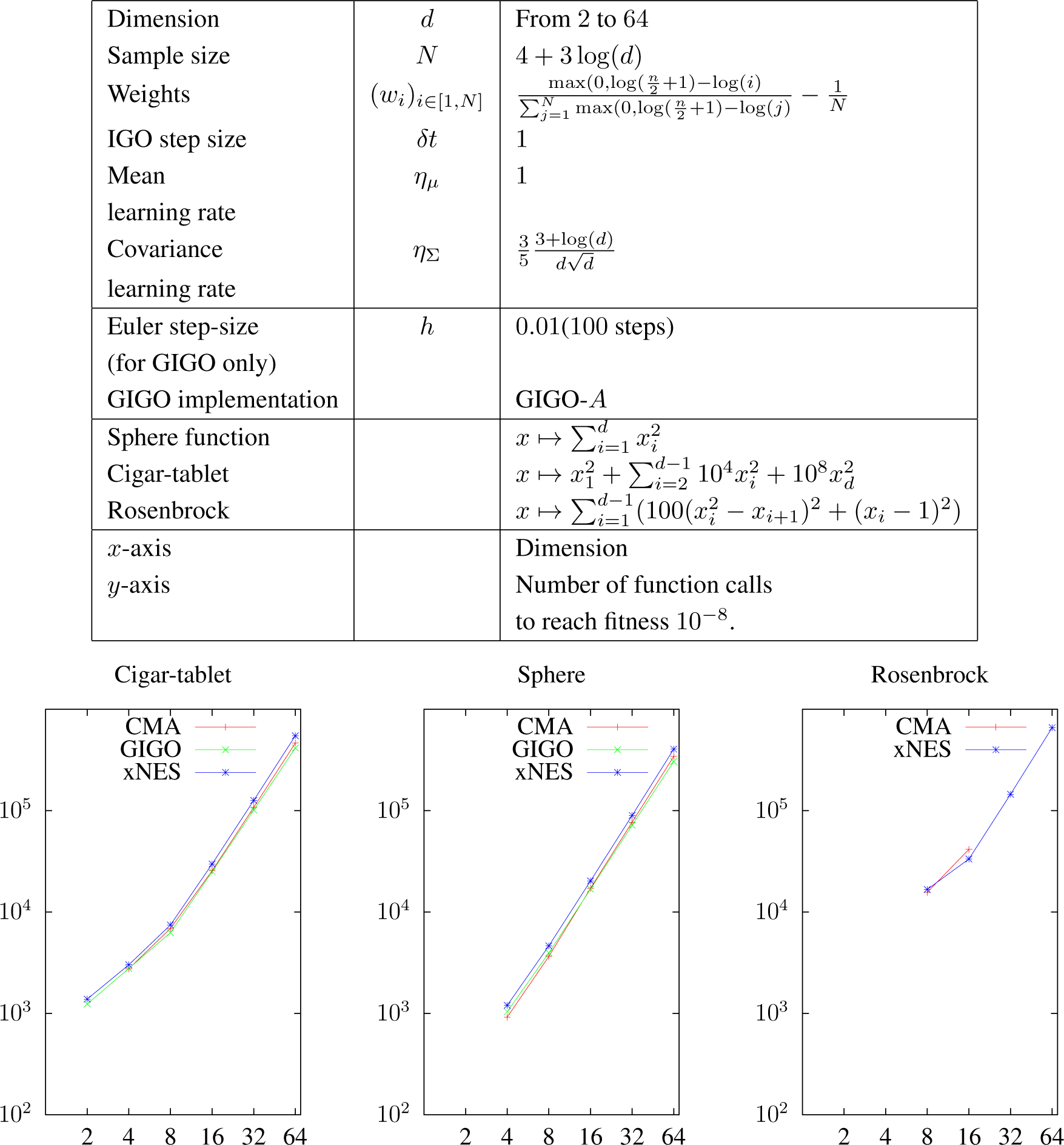
For the first series of experiments, presented in Figure 3, we used the following parameters, taken from [19] (we recall that xNES and pure rank-μ CMA-ES are seen as IGO algorithms):
- Varying dimension.
- Sample size:
- Weights: .
- IGO step size and learning rates: δt = 1, ημ = 1, ..
- Initial position: , where x0 is a random point of the circle with center zero, and radius 10.
- Euler method for GIGO: Number of steps: 100. We used the GIGO-A variant of the algorithm. No significant difference was noticed with GIGO-Σ or with the exact GIGO algorithm. The only advantage of having an explicit solution of the geodesic equations is that the update is quicker to compute.
- We chose not to use the exact expression of the geodesics for this benchmarking to show that having to use the Euler method is fine. However, we did run the tests, and the results are basically the same as GIGO-A.
We plot the median number of runs to achieve target fitness (10−8). Each algorithm has been tested in dimension 2, 4, 8, 16, 32 and 64: a missing point means that all runs converged prematurely.
7.1.1. Failed Runs
In Figure 3, a point is plotted even if only one run was successful. Below is the list of the settings for which at least one run converged prematurely.
- Only one run reached the optimum for the cigar-tablet function with CMA-ES in dimension eight.
- Seven runs (out of 24) reached the optimum for the Rosenbrock function with CMA-ES in dimension 16.
- About half of the runs reached the optimum for the sphere function with CMA-ES in dimension four.
For the following settings, all runs converged prematurely.
- GIGO did not find the optimum of the Rosenbrock function in any dimension.
- CMA-ES did not find the optimum of the Rosenbrock function in dimension 2, 4, 32 and 64.
- All of the runs converged prematurely for the cigar-tablet function in dimension two with CMA-ES, for the sphere function in dimension two for all algorithms and for the Rosenbrock function in dimension two and four for all algorithms.
7.1.2. Discussion
As the last item in Section 7.1.1 shows, all of the algorithms converge prematurely in a low dimension, probably because the covariance learning rate has been set too high (or because the sample size is too small). This is different from the results in [19].
This remark aside, as noted in [19], the xNES algorithm shows more robustness than CMA-ES and GIGO: it is the only algorithm able to find the minimum of the Rosenbrock function in high dimensions. However, its convergence is consistently slower.
In terms of performance, when both of them work, pure rank-μ CMA-ES (or equivalently, IGO in the parametrization (μ, Σ)) and GIGO are extremely close (GIGO is usually a bit better). An advantage of GIGO is that it is theoretically defined for any δt, ηΣ, whereas the covariance matrix maintained by CMA-ES (not only pure rank-μ CMA-ES) can stop being positive definite if ηΣδt > 1. However, in that case, the GIGO algorithm is prone to premature convergence (remember Figure 2 and see Proposition 15 below), and in practice, the learning rates are much smaller.
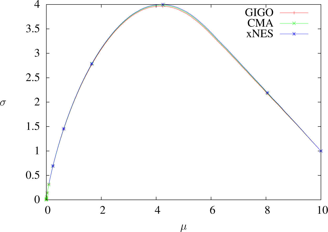
7.2. Plotting Trajectories in
We want the second series of experiments to illustrate the remarks about the trajectories of the algorithms in Section 6.3, so we decided to take a large sample size to limit randomness, and we chose a fixed starting point for the same reason. We use the weights below because of the property of quantile improvement proven in [23]: the 1/4-quantile will improve at each step. The parameters we used were the following:
- Sample size: λ = 5, 000
- Dimension one only.
- Weights: w = 41q⩽1/4 (wi = 4.1i⩽1,250)
- IGO step size and learning rates: ημ = 1, , varying δt.
- Initial position:
- Dots are placed at t = 0, 1, 2 … (except for the graph δt = 1.5, for which there is a dot for each step).
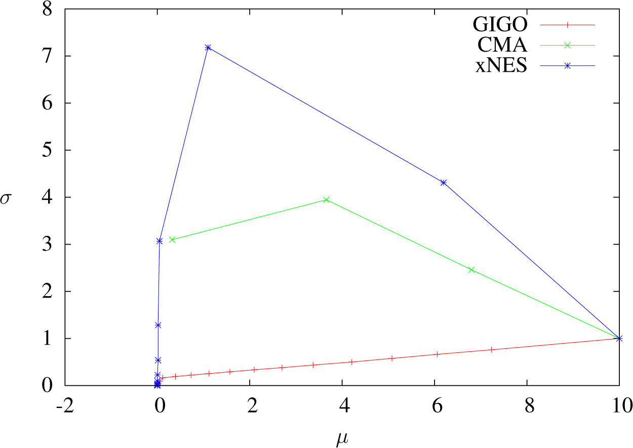
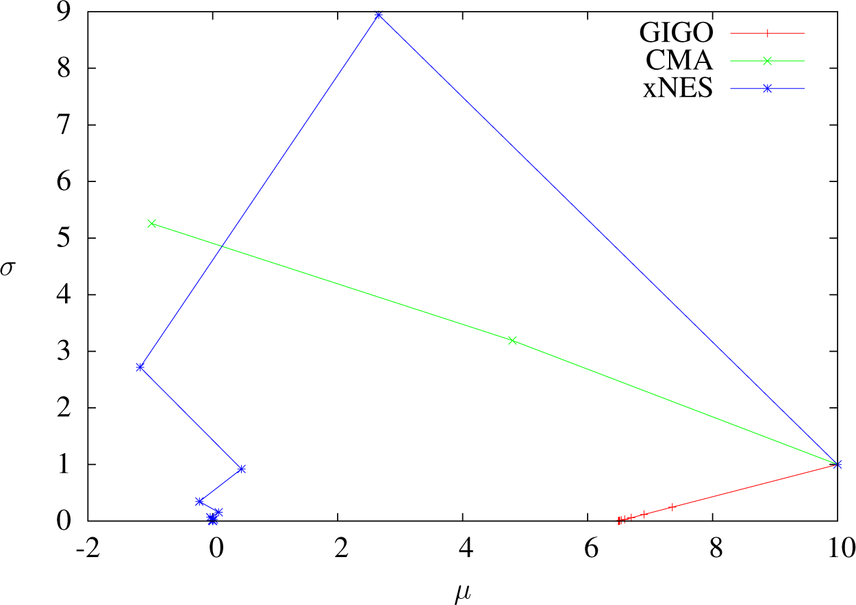
Figures 7, 8 and 11 show that when δt ≥ 1, GIGO reduces the covariance, even at the first step. More generally, when using the GIGO algorithm in
for the optimization of a linear function, there exists a critical step size δtcr (depending on the learning rates ημ, ησ and on the weights wi), above which, GIGO will converge, and we can compute its value when the weights are of the form
(for q0 ≥ 0.5, the discussion is not relevant, because in that case, even the IGO flow converges prematurely. Compare with the critical δt of the smoothed cross entropy method and IGO-ML in [1]).
Proposition 15. Let d ∈ ℕ, k, ημ,
; let and let
Let μn be the first coordinate of the mean, and let be the variance (at step n) maintained by the (ημ, ησ)-twisted geodesic IGO algorithm in associated with selection scheme w, sample size ∞ and step size δt, when optimizing g (“sample size ∞” meaning the limit of the update when the sample size tends to infinity, which is deterministic [1]).
There exists δtcr, such that:
- if δt > δtcr, (σn) converges to zero with exponential speed and (μn) converges.
- if δt = δtcr, (σn) remains constant and (μn) tends to ∞ with linear speed.
- if 0 < δt < δtcr, both (σn) and μn tend to ∞ with exponential speed.
The proof and the expression of δtcr can be found in the Appendix.
In the case corresponding to k = 4, n = 1, q0 = 1/4, ημ = 1, ησ = 1.8, we find:
8. Conclusions
We introduced the geodesic IGO algorithm, and we showed that in the case of Gaussian distributions, Noether’s theorem directly gives a first order equation satisfied by the geodesics. In terms of performance, the GIGO algorithm is similar to pure rank-μ CMA-ES, which is rather encouraging: it would be interesting to test GIGO on real problems. Moreover, GIGO is a reasonable and totally parametrization-invariant algorithm (provided we can compute the solution of the equations of the geodesics), and as such, it should be studied for other families of probability distributions, like Bernoulli distributions (although in that case, the Riemannian exponential is not defined if the step size is too large, because the length of the geodesics is finite). Noether’s theorem could be a crucial tool for this.
We also showed that xNES and GIGO are not the same algorithm, and we defined blockwise GIGO, a simple extension of the GIGO algorithm, showing that xNES has a special status, as it admits a definition that is “almost” parametrization-invariant.
Conflicts of Interest
The author declares no conflict of interest.
Proof of Proposition 15
Let us first consider the case k = 1.
When optimizing a linear function, the non-twisted IGO flow in
with the selection function
is known [1], and in particular, we have:
where, if we denote by
a random vector following a standard normal distribution and the cumulative distribution of a standard normal distribution,
and:
In particular,
and
.
With a minor modification of the proof in [1], we find that the (ημ, ησ)-twisted IGO flow is given by:
Notice that Equation (69) shows that the assertions about the convergence of (σn) immediately imply the assertions about the convergence of (μn).
Let us now consider a step of the GIGO algorithm: The twisted IGO speed is Y = (ημβσ0, ησασ0), with ασ0 > 0 (i.e., the variance should be increased: this is where we need q0 < 0.5).
Proposition 17 shows that the covariance at the end of the step is (using the same notation):
and it is easy to see that f only depends on δt (and on q0). In other words, f(δt) will be the same at each step of the algorithm. The existence of δtcr easily follows (furthermore, recall Figure 1 in Section 4.1), and δtcr is the positive solution of f(x) = 1.
After a quick computation, we find:
where:
and:
Finally, for
, Proposition 9 shows that:
A1. Generalization of the Twisted Fisher Metric
The following definition is a more general way to introduce the twisted Fisher metric.
Definition 17. Let (Θ, g) be a Riemannian manifold,
, a splitting (as defined in Section 6.4) of Θ compatible with the metric g.
We call (η1, …, ηn)-twisted metric on (Θ, g) for the splitting Θ1, …, Θn the metric g′ on Θ defined by for 1 ≤ i ≤ n, and Θi ⊥ Θj for i ≠ j.
Proposition 16. The (ημ, ηΣ)-twisted metric on with the Fisher metric for the splitting coincides with the (ημ, ηΣ)-twisted Fisher metric from Definition 11.
Proof. It is easy to see that the (ημ, ηΣ)-twisted Fisher metric satisfies the condition in Definition 17.
A2. Twisted Geodesics
The following theorem can be used to compute the twisted geodesics from the non twisted geodesics. It is a simple calculation.
Theorem 7. Let ημ, ηΣ ∈ ℝ, μ0 ∈ ℝd, A0 ∈ GLd(ℝ), and Let
We denote by ϕ (resp. ψ) the Riemannian exponential of (resp. with the (ημ, ηΣ)-twisted Fisher metric) at. We have:
Proof. Let us denote by:
the Fisher metric in the parametrization μ, Σ, and consider the 0 IΣ following parametrization of
.
The Riemannian exponential at
in this parametrization is:
However, in this parametrization, the Fisher metric reads:
which is proportional to the (ημ, ηΣ)-twisted Fisher metric up to a factor
. Consequently, the Christoffel symbols are the same as the Christoffel symbols of the (ημ, ηΣ)-twisted Fisher metric, and so are the geodesics. Therefore, we have:
which is what we wanted.
For the remainder of this section, we fix ημ and ηΣ;
is endowed with the (ημ, ηΣ)-twisted Fisher metric, and
is endowed with the induced metric. The proofs of the propositions below are a simple rewriting of their non-twisted counterparts that can be found in Sections 4 and 5.1 and can be seen as corollaries of Theorem 7.
Theorem 8. If is a twisted geodesic of, then there exists a, b, c, d ∈ ℝ, such that ad − bc = 1, and v > 0, such that, σ(t) = Im(γℂ(t)), with and:
Proposition 17. Let n ∈ ℕ, vμ ∈ ℝnr,vσ, ημ, ησ, σ0 ∈ ℝ, with σ0 > 0.
Let vr := ║vμ║
,
and.
Let and.
Let.
Then
is the twisted geodesic of satisfying γ(0) = (μ0, σ0) and. The regular geodesics of are obtained with ημ = ησ = 1.
Theorem 9. Let be a twisted geodesic of. Then, the following quantities are invariant:
Theorem 10. If μ : t ⟼ μt and Σ : t ⟼ Σt satisfy the equations:
where:
and:
then is a twisted geodesic of.
Theorem 11. If μ : t ⟼ μt and A : t ⟼ At satisfy the equations:
where:
and:
then is a twisted geodesic of.
A3. Pseudocodes
A3.1. For All Algorithms
All studied algorithms have a common part, given here:
Variables: μ, Σ (or A such that Σ = AAT).
List of parameters: f : ℝd → ℝ, step size δt, learning rates ημ, ηΣ, sample size λ, weights (wi)i∈[1,λ], N number of steps for the Euler method, r Euler step size reduction factor (for GIGO-Σ only).

 |
Notice that we always need a square root A of Σ to sample the xi, but the decomposition Σ = AAT is not unique. Two different decompositions will give two algorithms, such that one is a modification of the other as a stochastic process: same law (the xi are abstractly sampled from
, but different trajectories (for given zi, different choices for the square root will give different xi). For GIGO-Σ, since we have to invert the covariance matrix, we used the Cholesky decomposition (A lower triangular. The the other implementation directly maintains a square root of Σ). Usually, in CMA-ES, the square root of Σ (Σ = AAT, A symmetric) is used.
A3.2. Updates
When describing the different updates, μ, Σ, A, the xi and the zi are those defined in Algorithm 1. For Algorithm 2 (GIGO-Σ), when the covariance matrix after one step is not positive-definite, we compute the update again, with a step size divided by r for the Euler method (we have no reason to recommend any particular value of r, the only constraint is r > 1).
 |
 |
Algorithm 4.
Exact GIGO, one step. Not exactly our implementation; see the discussion after Corollary 1.
 |
 |
 |
 |
Acknowledgments
I would like to thank Yann Ollivier for his numerous remarks about this article and Frédéric Barbaresco for finding [5].
References
- Ollivier, Y.; Arnold, L.; Auger, A.; Hansen, N. Information-geometric optimization algorithms: A unifying picture via invariance principles 2011, arXiv, 1106.3708.
- Amari, S.-I.; Nagaoka, H. Methods of Information Geometry (Translations of Mathematical Monographs); American Mathematical Society: Providence, RI, USA, 2007. [Google Scholar]
- Malagò, L.; Pistone, G. Combinatorial optimization with information geometry: The Newton method. Entropy 2014, 16, 4260–4289. [Google Scholar]
- Eriksen, P. Geodesics Connected with the Fisher Metric on the Multivariate Normal Manifold; Technical Report 86-13; Institute of Electronic Systems, Aalborg University: Aalborg, Denmark, 1986. [Google Scholar]
- Calvo, M.; Oller, J.M. An Explicit Solution of Information Geodesic Equations for the Multivariate Normal Model. Stat. Decis. 1991, 9, 119–138. [Google Scholar]
- Imai, T.; Takaesu, A.; Wakayama, M. Remarks on geodesics for multivariate normal models. J. Math-for-Industry 2011, 3, 125–130. [Google Scholar]
- Skovgaard, L.T. A Riemannian geometry of the multivariate normal model. Scand. J. Stat. 1981, 11, 211–223. [Google Scholar]
- Porat, B.; Friedlander, B. Computation of the Exact Information Matrix of Gaussian Time Series with Stationary Random Components. IEEE Trans. Acoust. Speech Signal Process 1986, 34, 118–130. [Google Scholar]
- Baluja, S.; Caruana, R. Removing the Genetics from the Standard Genetic Algorithm; Technical Report CMU-CS-95-141; Morgan Kaufmann Publishers: Burlington, MA, USA, 1995; pp. 38–46. [Google Scholar]
- Malagò, L.; Matteucci, M.; Pistone, G. Towards the geometry of estimation of distribution algorithms based on the exponential family, Proceedings of the 11th Workshop Proceedings on Foundations of Genetic Algorithms, Schwarzenberg, Austria, 5–9 January 2011; pp. 230–242.
- Kern, S.; Müller, S.D.; Hansen, N.; Büche, D.; Ocenasek, J.; Koumoutsakos, P. Learning probability distributions in continuous evolutionary algorithms—A comparative review. Nat. Comput. 2003, 3, 77–112. [Google Scholar]
- Wierstra, D.; Schaul, T.; Glasmachers, T.; Sun, Y.; Peters, J.; Schmidhuber, J. Natural evolution strategies. J. Mach. Learn. Res. 2014, 15, 949–980. [Google Scholar]
- Huang, W. Optimization Algorithms on Riemannian Manifolds with Applications. Ph.D. Thesis, Florida State University, Tallahassee, FL, USA, 2013. [Google Scholar]
- Absil, P.A.; Mahony, R.; Sepulchre, R. Optimization Algorithms on Matrix Manifolds; Princeton University Press: Princeton, NJ, USA, 2008. [Google Scholar]
- Arnold, V.; Vogtmann, K.; Weinstein, A. Mathematical Methods of Classical Mechanics (Graduate Texts in Mathematics); Springer: New York, NY, USA, 1989. [Google Scholar]
- Bourguignon, J. Calcul variationnel; Ecole Polytechnique: Palaiseau, France, 2007; in French. [Google Scholar]
- Jost, J.; Li-Jost, X. Calculus of Variations (Cambridge Studies in Advanced Mathematics); Cambridge University Press: Cambridge, UK, 1998. [Google Scholar]
- Gallot, S.; Hulin, D.; LaFontaine, J. Riemannian Geometry (Universitext), 3rd ed; Springer: Berlin/Heidelberg, Germany, 2004. [Google Scholar]
- Glasmachers, T.; Schaul, T.; Yi, S.; Wierstra, D.; Schmidhuber, J. Exponential natural evolution strategies, Proceedings of the 12th Annual Conference on Genetic and Evolutionary Computation, Portland, OR, USA, 7–11 July 2010.
- Akimoto, Y.; Nagata, Y.; Ono, I.; Kobayashi, S. Bidirectional relation between CMA evolution strategies and natural evolution strategies. In Parallel Problem Solving from Nature, PPSN XI; Schaefer, R., Cotta, C., Kołodziej, J., Rudolph, G., Eds.; Springer: New York, NY, USA, 2010. [Google Scholar]
- Hansen, N. The CMA evolution strategy: A tutorial. Available online: https://www.lri.fr/∼hansen/cmatutorial.pdf accessed on 1 January 2015.
- Bensadon, J. Source Code. Available online: https://www.lri.fr/~bensadon/ accessed on 13 January 2015.
- Akimoto, Y.; Ollivier, Y. Objective improvement in information-geometric optimization, Proceedings of the twelfth workshop on Foundations of genetic algorithms XII, Adelaide, Australia, 16–20 January 2013.
Figure 1.
Geodesics of the Poincaré half-plane.

Figure 2.
One step of the geodesic IGO (GIGO) update.

Figure 3.
Median number of function calls to reach 10−8 fitness on 24 runs for: sphere function, cigar-tablet function and Rosenbrock function. Initial position θ0 = N (x0, I), with x0 uniformly distributed on the circle of center zero and radius 10. We recall that the “CMA-ES” algorithm here is using the so-called pure rank-μ CMA-ES update.

Figure 4.
Trajectories of GIGO, CMA and xNES optimizing x ↦ x2 in dimension one with δt = 0.01, sample size 5000, weights wi = 4.1i⩽1250 and learning rates ημ = 1, ηΣ = 1.8. One dot every 100 steps. All algorithms exhibit a similar behavior
Figure 4.
Trajectories of GIGO, CMA and xNES optimizing x ↦ x2 in dimension one with δt = 0.01, sample size 5000, weights wi = 4.1i⩽1250 and learning rates ημ = 1, ηΣ = 1.8. One dot every 100 steps. All algorithms exhibit a similar behavior

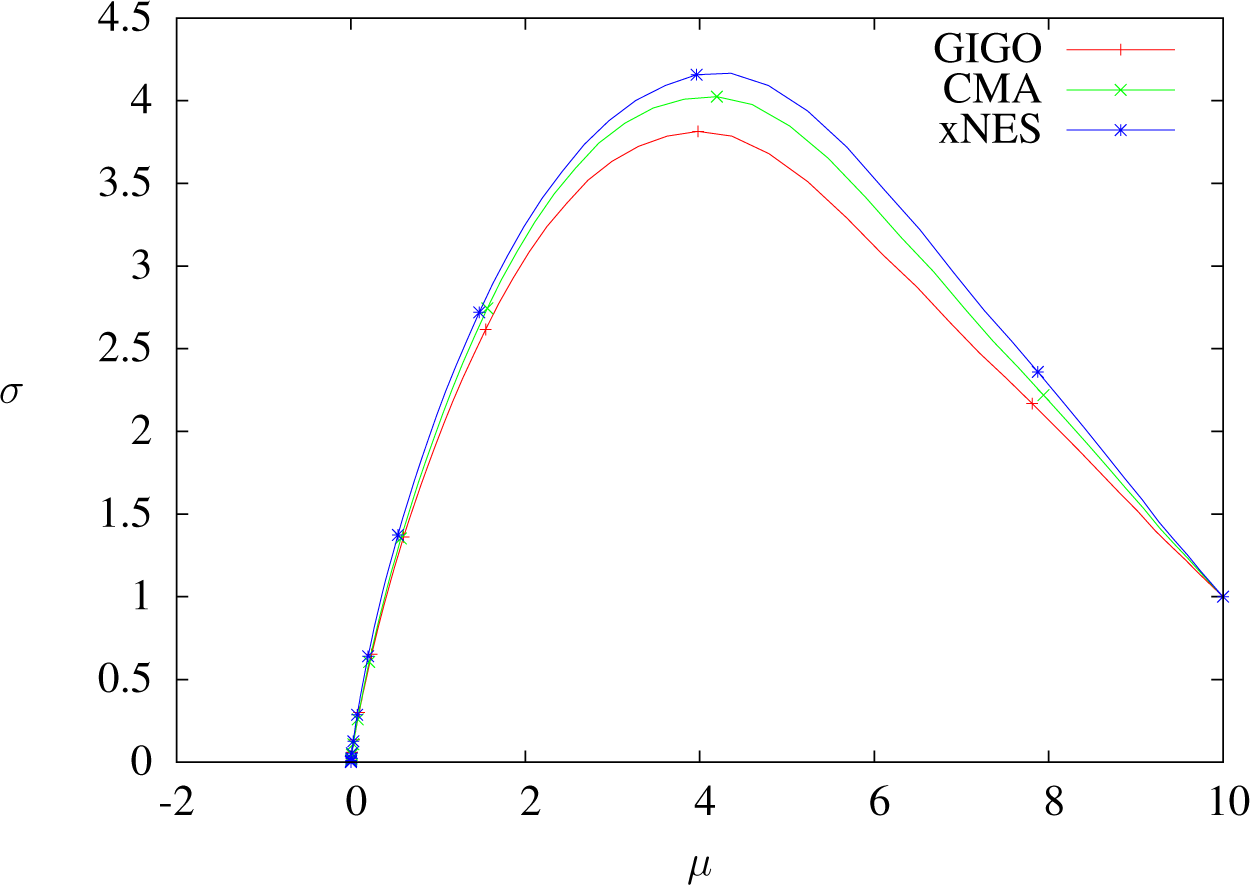
Figure 5.
Trajectories of GIGO, CMA and xNES optimizing x 7→x2 in dimension one with δt = 0.5, sample size 5000, weights wi = 4.1i⩽1250 and learning rates ημ = 1, ηΣ = 1.8. One dot every two steps. Stronger differences. Notice that after one step, the lowest mean is still GIGO (∼ 8.5, whereas xNES is around 8.75), but from the second step, GIGO has the highest mean, because of the lower variance.

Figure 6.
Trajectories of GIGO, CMA and xNES optimizing x ⟼ x2 in dimension one with δt = 0.1, sample size 5000, weights wi = 4.1i≤1250 and learning rates ημ = 1, ηΣ = 1.8. One dot every 10 steps. All algorithms exhibit a similar behavior, and differences start to appear. It cannot be seen on the graph, but the algorithm closest to zero after 400 steps is CMA (∼ 1.10−16, followed by xNES (∼ 6.10−16) and GIGO (∼ 2.10−15).

Figure 7.
Trajectories of GIGO, CMA and xNES optimizing x ⟼ x2 in dimension one with δt = 1, sample size 5000, weights wi = 4.1i≤1250 and learning rates ημ = 1, ηΣ = 1.8. One dot per step. The CMA-ES algorithm fails here, because at the fourth step, the covariance matrix is not positive definite anymore (it is easy to see that the CMA-ES update is always defined if δtηΣ < 1, but this is not the case here). Furthermore, notice (see also Proposition 15) that at the first step, GIGO decreases the variance, whereas the σ-component of the IGO speed is positive.

Figure 8.
Trajectories of GIGO, CMA and xNES optimizing x ⟼ x2 in dimension one with δt = 1.5, sample size 5000, weights wi = 4.1i≤1250 and learning rates ημ = 1, ηΣ = 1.8. One dot per step. Same as δt = 1 for CMA. GIGO converges prematurely.
Figure 8.
Trajectories of GIGO, CMA and xNES optimizing x ⟼ x2 in dimension one with δt = 1.5, sample size 5000, weights wi = 4.1i≤1250 and learning rates ημ = 1, ηΣ = 1.8. One dot per step. Same as δt = 1 for CMA. GIGO converges prematurely.

Figure 9.
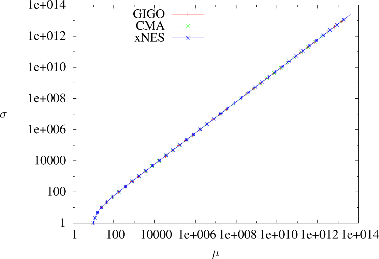
Trajectories of GIGO, CMA and xNES optimizing x ⟼ −x in dimension one with δt = 0.01, sample size 5000, weights wi = 4.1i≤1250 and learning rates ημ = 1, ηΣ = 1.8. One dot every 100 steps. Almost the same for all algorithms.
Figure 9.
Trajectories of GIGO, CMA and xNES optimizing x ⟼ −x in dimension one with δt = 0.01, sample size 5000, weights wi = 4.1i≤1250 and learning rates ημ = 1, ηΣ = 1.8. One dot every 100 steps. Almost the same for all algorithms.

Figure 10.
Trajectories of GIGO, CMA and xNES optimizing x ⟼ −x in dimension one with δt = 0.1, sample size 5000, weights wi = 4.1i≤1250 and learning rates ημ = 1, ηΣ = 1.8. One dot every 10 steps. It is not obvious on the graph, but xNES is faster than CMA, which is faster than GIGO.
Figure 10.
Trajectories of GIGO, CMA and xNES optimizing x ⟼ −x in dimension one with δt = 0.1, sample size 5000, weights wi = 4.1i≤1250 and learning rates ημ = 1, ηΣ = 1.8. One dot every 10 steps. It is not obvious on the graph, but xNES is faster than CMA, which is faster than GIGO.

Figure 11.
Trajectories of GIGO, CMA and xNES optimizing x ⟼ −x in dimension one with δt = 1, sample size 5, 000, weights wi = 4.1i≤1,250 and learning rates ημ = 1, ηΣ = 1.8. One dot per step. GIGO converges, for the reasons discussed earlier.
Figure 11.
Trajectories of GIGO, CMA and xNES optimizing x ⟼ −x in dimension one with δt = 1, sample size 5, 000, weights wi = 4.1i≤1,250 and learning rates ημ = 1, ηΣ = 1.8. One dot per step. GIGO converges, for the reasons discussed earlier.

© 2015 by the authors; licensee MDPI, Basel, Switzerland This article is an open access article distributed under the terms and conditions of the Creative Commons Attribution license (http://creativecommons.org/licenses/by/4.0/).
Share and Cite
MDPI and ACS Style
Bensadon, J. Black-Box Optimization Using Geodesics in Statistical Manifolds. Entropy 2015, 17, 304-345. https://0-doi-org.brum.beds.ac.uk/10.3390/e17010304
AMA Style
Bensadon J. Black-Box Optimization Using Geodesics in Statistical Manifolds. Entropy. 2015; 17(1):304-345. https://0-doi-org.brum.beds.ac.uk/10.3390/e17010304
Chicago/Turabian StyleBensadon, Jérémy. 2015. "Black-Box Optimization Using Geodesics in Statistical Manifolds" Entropy 17, no. 1: 304-345. https://0-doi-org.brum.beds.ac.uk/10.3390/e17010304