Entropy-Based Characterization of Internet Background Radiation

Abstract

Network security requires real-time monitoring of network traffic in order to detect new and unexpected attacks. Attack detection methods based on deep packet inspection are time consuming and costly, due to their high computational demands. This paper proposes a fast, lightweight method to distinguish different attack types observed in an IP darkspace monitor. The method is based on entropy measures of traffic-flow features and machine learning techniques. The explored data belongs to a portion of the Internet background radiation from a large IP darkspace, i.e., real traffic captures that exclusively contain unsolicited traffic, ongoing attacks, attack preparation activities and attack aftermaths. Results from an in-depth traffic analysis based on packet headers and content are used as a reference to label data and to evaluate the quality of the entropy-based classification. Full IP darkspace traffic captures from a three-week observation period in April, 2012, are used to compare the entropy-based classification with the in-depth traffic analysis. Results show that several traffic types present a high correlation to the respective traffic-flow entropy signals and can even fit polynomial regression models. Therefore, sudden changes in traffic types caused by new attacks or attack preparation activities can be identified based on entropy variations.

1. Introduction

The difficulties in classifying, modeling and simulating network traffic from global perspectives have been frequently documented in the scientific literature. Some of the main reasons behind the challenges are the high heterogeneity of communication networks, their continuously evolving nature and the proliferation of techniques to avoid traffic being identified [1,2]. To say that we do not have suitable models to represent big-scale Internet traffic means to accept a disturbing lack of background understanding in a field whose relevance is out of the question. This lack has an obvious impact on the performance and efficiency at every level of the design of wide area communication networks and especially for network security and the detection of attacks.

There are many tools that are able to identify traffic types by means of a deep exploration of captured packets, e.g., Bro [3], PACE (protocol and application classification with metadata extraction) [4] and NBAR (network-based application recognition) [5]. Such tools provide useful and reliable traffic classifications, but they require costly packet inspections that hamper their usage for real-time large-scale monitoring purposes. This is a problem in situations where network observation and analysis need to promptly detect and react against extended failures or spreading threats. Moreover, inspecting payload data must deal with increasingly restrictive privacy policies, as well as encryption, tunneling and protocol obfuscation. The proposed entropy-based method does not require payload inspection and, thus, is also applicable in scenarios where payload is not available.

From the information theory perspective, it is possible to find dependencies between network traffic types and the distributions of traffic features (such as addresses, port numbers, etc.), especially for traffic generated by attackers or victims of attacks. The reason for this is that attackers often use either random values or one very specific value when launching an attack. One example is the use of randomly spoofed source addresses by attackers to conceal their own identity or to pretend that requests originate from multiple machines, so that the victim starts sending a lot of responses to different destinations. Another example for random values in attacks is scanning activities, which randomly scan IP addresses or port numbers. While random sources or destinations lead to a dispersion of traffic features, targeted attacks to specific addresses or ports lead to a concentration in the distribution of a feature. The dispersion and concentration of features are clearly visible in the feature distributions and, therefore, influence the entropy. Thus, the detection of events involving random or specific values is possible based on entropy without inspecting packet content.

Shannon entropy provides a lightweight compact representation of traffic feature distributions in order to characterize network events (e.g., [6,7]). Darkspace data are well suited for entropy-based analysis, since they only consist of unsolicited traffic, which predominantly contains random or specific traffic features [8]. In Section 2, we summarize related work in which network anomalies and attacks are identified by measuring the distribution properties of flow features.

In this paper, we examine a dataset corresponding to Internet background radiation (IBR) measured at a large IP darkspace. A darkspace is formed by an IP address range that does not contain real hosts, i.e., empty addresses that neither request communication nor answer incoming communication attempts. In theory, no traffic should arrive at the darkspace, yet it actually does. All of these arriving packets are therefore undesired and originate mainly from misconfiguration, attacks, attack preparations and their aftermaths. Furthermore, communication to a darkspace is always unidirectional, because there are no hosts that can originate or answer requests; as a consequence, it is also not possible to establish a TCP connection to a darkspace address. TCP packets in the darkspace correspond only to connection attempts and responses to connection attempts outside the darkspace that were sent with spoofed source addresses (e.g., SYN or RST packets from victims responding to SYNs with spoofed source addresses).

In spite of not being a radiation strictly speaking, the term “Internet background radiation” (IBR) has been coined due to the fact that the data observed in darkspaces contain persistent traffic that originates from many sources distributed all over the world [9]. Due to the global distribution of sources sending to the darkspace, IBR provides a valuable source for Internet situational awareness from a global perspective. Darkspace traffic has been used extensively to study global spreading of malware (e.g., [10–13]), analyzing large-scale coordinated attacks [14] and effects from globally-synchronized patching efforts [15]. It also provides valuable input to study events with global impact on Internet connectivity, such as country-wide or regional network outages due to natural disasters, technical problems or censorship [16]. Several application fields for the use of darkspace data are reported in [17].

This paper aims at the improvement of the state of the art in four ways:

• Proposing entropy-based models for the IBR traffic analysis as a basis for a fast and lightweight recognition of new malicious events in wide area networks.
• Discovering correlations between anomalous traffic types detected with deep inspection techniques and traffic feature entropy variations.
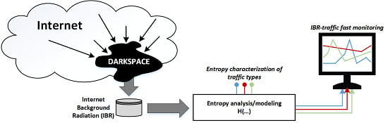
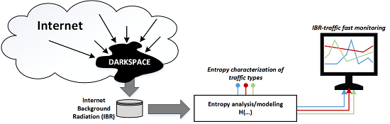
• Providing a traffic-type dissection (in-depth and entropy based) of a representative portion of the IBR for three weeks of April, 2012, with a 10-minute time scope.
• Providing an entropy-based detection method to discover anomalies in the IBR for early warning purposes.

To do that, we analyze three-week data from a/8 darkspace monitor, which corresponds to 1/256 of the entire IPv4 address space, and study the time series corresponding to traffic types obtained by means of deep packet inspection and the entropy signals of traffic-flow features. The darkspace data are provided by the Center for Applied Internet Data Analysis (CAIDA) at the University of California, San Diego (UCSD), CA, USA [18]. For the deep analysis, we deploy the most recent release of the corsaro software suite [19] with the smee plug-in, which categorizes traffic into 17 classes. Corsaro has been specifically devised for the analysis of darkspace traffic and allows aggregation with regard to different traffic features. Traffic types are explained in Section 3. Entropy analysis of traffic-flow features is detailed in Section 4. We explore dependencies and the correlation between both sets of signals by means of different machine learning and mathematical approaches. The experiments and modeling processes are introduced in Section 5. Results are shown in Section 6. The main findings are discussed in detail in Section 7. Conclusions are provided in Section 8.

It is important to remark that it is not possible to decouple the effect of isolated traffic types from the global entropy measures. As for the fast-monitoring schemes, this means that periodical tuning of fast detectors with feedback from a deep, parallel analysis of selected parts of the traffic is required to correctly adapt to the changing nature of network traffic. With regard to the models, it entails that they are accurate as long as traffic type signals keep a certain stationarity. If the average proportions of traffic types evolve over time, models must be re-calculated, even though the discovered dependency relationships continue being valid in a broad sense. For example, results show that TCP scanning to port 445 has an obvious impact on the overall entropy of the globally-used destination ports. This is detectable because TCP scanning to port 445 is a widespread phenomenon that occurs very often and covers a considerable portion of the global traffic. If for any reason TCP scanning to port 445 becomes an obsolete practice, its average rate will decrease, affecting the whole picture of traffic types. Hence, predictive models must be tuned to fit the new network reality and its impact on the overall entropy signals.

2. Related Work

Payload encryption, privacy concerns and the necessity of lightweight, fast analysis methods suggest that the future of network traffic classification leans toward the usage of flow-traffic data rather than toward payload inspection. Unsupervised classification methodologies processing vectors based on flow-traffic features have actually shown a similar detection power as classic deep packet inspection approaches [2].

Using flow-traffic features is lighter, but it does not necessarily involve a light detection system. It depends on the specific methodology, i.e., methods that collect and process flow data for every specific source or destination during a fixed time interval can still be quite demanding in computational terms. For instance, an exhaustive exploration is conducted in [20], where traffic is classified by a two-step procedure: first, establishing TCP, UDP and ICMP session models and, later, detecting activity profiles that match predefined patterns based on the flow-traffic information observed during a time interval. After analyzing almost 10 million incoming sessions, the authors find out that 98.6% of the traffic matches the proposed activity patterns. Furthermore, in [21], DoS/DDoS attacks are detected based on expected forms of flow headers and characteristic behaviors in other traffic-flow parameters that are aggregated and examined after a predetermined rate.

As for entropy measures, in the related literature we find that they are applied to traffic analysis in different ways. In [6], the authors calculate four entropy time series for every existing OD (origin-destination) flow pair between PoP (points-of-presence) in the Abilene and Gèant backbone network. The flow features are: source IP, destination IP, source port and destination port. The input space is transformed and expressed in vectors, which are processed by unsupervised classifiers and, therefore, clustered. Similarly and using the same datasets, in [22], the authors propose nonextensive entropy, a one-parameter generalization of Shannon entropy, and show that this method outperforms classic entropy-based methods. The computational costs, scalability and suitability of such entropy-based methods are strongly tied to the number of PoPs considered. Entropy measures are applied differently in [23], where anomalies are detected by comparing ongoing traffic with a baseline distribution. Traffic is filtered and classified according to 2348 packet classes that are established based on flow headers. Detection algorithms are based on maximum entropy and relative entropy estimations of the given classes. The authors affirm that entropy-based measures require a computation time proportional to the traffic rate and are also useful to provide images of the current network traffic. Finally, a generalized form of entropy is calculated for six flow features corresponding to the whole network in [7]. Here, the authors introduce the traffic entropy spectrum (TES) for the sensitive, fast processing of a high amount of data points. Since in our work we do not aim at the identification of attacks at a specific packet or OD level, but at the characterization of aggregated network flows, our approach is closer to this last referred work. We sacrifice granularity in the detection to gain simplicity and swiftness. Our approach does not classify the specific anomalous piece of traffic, but guides deeper, subsequent detection by first filtering and reading of the traffic context.

We specifically focus on the darkspace in order to obtain a better understanding of anomalies and their imprints or profiles. The characteristics of the IBR have been explored in [24] by checking the traffic of four large IP darkspace monitors. Given the huge amount of incoming traffic, the authors devise a filtering scheme that keeps traffic variety and builds an application-level responder framework that helps to characterize processed packets. They discover a general preponderance of TCP SYN-ACK/RST packets in backscatter traffic, but no other clear trend in the analyzed subnets, emphasizing the extreme dynamism of background radiation. Six years later, the IBR is revisited in [9] by analyzing an unused/8 network and three/8 recently allocated subnets. Results show that background traffic continues to be highly dynamic and varied; however, they detect new trends in the exploitation of specific ports, increasing of SYN and decreasing of SYN-ACK traffic. In addition, they suggest that there is a dominant growth of traffic pollution due to misconfiguration and environmental factors, rather than algorithmic sources. In [13], the authors present a taxonomy for one-way traffic sources using two classification perspectives: 14 source types based on Treurinet schemes [20] and 10 groups based on measures on inter-arrival time distributions. In [25], the authors detect malicious traffic behaviors in the darkspace by means of non-parametric sliding window techniques, which do not require any knowledge about the probability distribution of the underlying processes. Finally, in [8], entropy-based metrics prove to be useful to discover relevant events for IP darkspace: multi-source scans, backscatter and large probing.

We foresee that complete, flexible network detection schemes must face the problem in a heterogeneous way, i.e., by different perspectives and approaching different phases and steps. In this regard, in [24], the authors faced a huge amount of incoming traffic to process and analyze, so they opted to filter part of the traffic, which was directly dropped. Even though the filter was optimized to minimize the significance lost, some traffic remained unprocessed. Instead, a first, quick monitoring of the network can guide, select and tune subsequent detection phases. Note that a large amount of the IBR belongs to well-known, less relevant traffic, which must be identified and classified, but where deep analysis becomes a costly drain of computational resources. For instance, in a recent work [26], by using clustering techniques on flow-traffic features, we discovered a set of very stable dominant patterns that accounts for 75% of the darkspace traffic sources; therefore, it is possible to quickly label 75% of the sources as known traffic and concentrate the deeper analysis on the remaining 25%.

3. Deep Packet Inspection

This chapter describes the in-depth packet inspection performed to establish a baseline labeling of the data.

3.1. Dataset

The experiments conducted throughout the current paper deploy a portion of traffic from a large/8 darkspace monitor operated at the University of California, San Diego (UCSD) [18]. The considered time period covers April 8, 2012, 12:00 UTC, to May 1, 2012, 00:00 UTC. Complete traffic traces have been captured and stored in pcap files. Due to some gaps in the captured files, we did not include the first week of April, 2012, in our analysis.

3.2. Obtaining Traffic Types

In order to obtain traffic type signals, the corsaro tool is used with the smee plug-in, which is able to perform a deep packet inspection analysis using the libraries and algorithms of the IATmon tool [13]. In the following, we refer to traffic types or smee types to denote the labels that are applied to the data by performing the in-depth analysis with the smee plug-in (smee analysis).

The measurement interval for the analysis is 10 min. Packets observed in each 10-minute observation period are first sorted according to the source IP address used in the packet. Then, all packets that originate from the same source IP address (within the 10-minute period) are analyzed. Based on this analysis, the traffic type (sent by the source) is determined. For instance, a source sending only ICMP packets within the 10-minute interval is labeled as an icmpOnly source. The classification of packets is based on the source classification and not only on the packet characteristics. Each packet is assigned to exactly one traffic type. All packets sent by sources of type icmpOnly are classified as packets of type icmpOnly. As a consequence, a UDP packet can belong to one of several different traffic type (e.g., udpHscan or udpVscan), depending on the behavior of the source from which the packet originated. Additionally, note the term “unique” for the sources in Figure 1, indicating that every different source IP is only counted once regardless of the number of packets it sends during the 10-minute interval.

The output of the smee analysis is summary files, where packets and sources from the input pcap file are classified and aggregated according to predefined smee traffic types. By parsing the report files with Perl scripts, smee types are finally arranged in tables and subsequently in time series. Every table sample (row) follows the format shown in Listing 1 (“pkts” and “srcs” stand for “packets” and “sources”, respectively, n = 17 smee traffic types). time_bin_ID identifies every analyzed 10-minute time interval and pkts_type_i shows how many packets of a specific traffic type i were observed in this interval. Analogously, src_type_i shows how many sources are originating traffic of traffic type i in the 10-minute interval.

A schema of the conducted process is shown in Figure 2; obtained time series are displayed in Figure 1.

Listing 1:. Smee result format.

Listing 1:. Smee result format.

3.3. Smee Types

Smee types are described below. In the remainder of the paper, we refer to them by the abbreviated form introduced here. Definitions are valid to classify both: the sources that send the given type of traffic and the packets that match the respective definition. The number of sources defines the unique number of source IP addresses that originate the specific traffic class. The packet count for a specific class is the total number of packets from all sources (in the time interval) that send this kind of traffic. For example, if three unique sources send two packets each, the source count for the class 1or2pkts is three sources and the packet count for the class 1or2pkts is six packets. The traffic classes are mutually exclusive. That means a source is assigned to the most detailed description.

• One or two packets (1or2pkts): a source that only sends one or two packets during the selected time interval (10 min), regardless of the protocol, destination IP or destination port. That means sources of all other classes send at least three packets.
• Unclassified traffic (unclass): packets and sources that do not match any of the following classes.
• TCP probe (tcpProb): a source that sends TCP packets to one destination IP and one destination port.
• TCP vertical scan (tcpVscan): a source that sends TCP packets to multiple destination ports of the same destination IP.
• TCP horizontal scan (tcpHscan): a source that sends TCP packets to the same port of multiple destination IPs (except to port 445).
• TCP unknown (tcpUnk): a source that sends TCP packets to multiple ports of multiple destination IPs.
• UDP probe (udpProb): a source that sends UDP packets to one destination IP and one destination port.
• UDP vertical scan (udpVscan): a source that sends UDP packets to multiple destination ports of the same destination IP.
• UDP horizontal scan (udpHscan): a source that sends UDP packets to the same port of multiple destination IPs.
• UDP unknown (udpUnk): a source that sends UDP packets to multiple ports of multiple destination IPs.
• ICMP only (icmpOnly): a source that only sends ICMP messages.
• TCP and UDP (tcp&udp): a source that sends both TCP and UDP packets during the checked time interval.
• μTorrent (uTorrent): a source that sends packets that fit the μTorrent packet profile. The μTorrent packets are identified in smee by analyzing the UDP packet payload.
• Conficker.C (confickC): a source that sends packets that fit a specific P2P packet format, which is used by the Conficker.C worm for spreading to other victims. For identifying Conficker.C P2P packets, smee uses the algorithm presented in [27].
• TCP backscatter (tcpBacks): a source that sends TCP packets with ACK or RST flags.
• DNS backscatter (dnsBacks): a source that sends TCP or UDP packets from the source port 53.
• TCP horizontal scan to port 445 (tcp445scan): a source that sends TCP packets to port 445 of multiple destination IPs.

3.4. Analysis of Smee Time Series

Some statistics are provided in

Table 1. Characteristics of smee type time series.

Number of PACKETS	mean*	SD*	hourly per.	half-day per.	daily per.	weekly per.	Significant peaks**
unclass	1.3 M	1.2 M	—	—	—	—	750, some
tcpProb	0.6 M	0.2 M	x	—	x	—	1702
tcpVscan	0.1 M	0.1 M	x	—	x	—	1295, 2021, 1294, some
tcpHscanP	34.6 M	38.2 M	—	x	—	—	509, 269, several
tcpUnk	14.4 M	10.8 M	—	—	x	—	1634
udpProb	6.3 M	1.3 M	—	—	—	x	3100
udpVscanP	11.4 M	5.1 M	—	—	—	x	2654
udpHscan	4.8 M	2.9 M	—	—	x	—	774
udpUnk	7.5 M	2.9 M	—	—	—	x	—
icmpOnlyP	7.5 M	2.5 M	—	x	—	x	542, 355
tcp&udp	3.8 M	3.1 M	x	x	x	—	1169
uTorrentP	2.4 M	0.7 M	—	—	x	—	—
confickC	0.6 M	1.4 M	—	—	x	—	2698
1or2pktsP	0.5 M	0.3 M	—	x	x	—	364
tcpBacksP	61.9 M	28.4 M	—	—	—	x	several
dnsBacks	0.9 M	0.7 M	—	—	—	—	717
tcp445scanP	86.0 M	17.9 M	—	—	x	—	—
# unique SOURCES	mean*	SD*	hourly per.	half-day per.	daily per.	weekly per.	significant peaks**
unclass	1.0 K	0.8 K	x	—	—	—	unequal periods
tcpProb	17.0 K	4.2 K	x	—	x	—	2526, 1758
tcpVscan	1.0 K	0.5 K	x	—	x	—	—
tcpHscan	30.3 K	8.4 K	x	—	x	—	unequal last period
tcpUnk	7.6 K	2.7 K	x	—	x	—	—
udpProbS	37.3 K	22.2 K	x	x	x	—	—
udpVscanS	1.2 K	0.8 K	x	x	x	—	—
udpHscanS	2.9 K	1.9 K	x	x	x	—	—
udpUnkS	61.1 K	54.4 K	x	x	x	—	366
icmpOnly	5.3 K	2.1 K	—	—	x	x	1590, unequal periods
tcp&udpS	12.9 K	4.0 K	x	—	x	—	—
uTorrentS	19.5 K	6.8 K	x	—	x	—	444
confickC	12.8 K	2.3 K	x	—	x	—	—
1or2pktsS	69.9 K	48.1K	x	x	x	—	366
tcpBacks	0.3 K	0.2 K	x	—	x	—	1344, 786
dnsBacks	31.2	9.7	x	—	—	—	—
tcp445scanS	86.0 K	21.3 K	x	—	x	—	—

^*per 10 min;

^**values correspond to sample IDs (timely ordered). Every sample covers 10 min of analyzed traffic;

^P,S: liable to be modeled by entropy measures of traffic-flow data (P-packets, S-sources), Section 6; SD: standard deviation; per.: periodicity; x: outstanding; —: nonexistent or negligible; M: Mega; K: Kilo.

and

Table 2. Percentage and packets/source of smee classes in the analyzed dataset. pkts, packets; src, source.

Smee class	packets (total)	packets (per 10 min)	sources (per 10 min)	pkts/src
unclass	0.5%	0.5% ± 0.46%	0.3% ± 0.24%	0.8 K±0.8 K
tcpProb	0.2%	0.2% ± 0.08%	5.0% ± 1.60%	3.7±1.9
tcpVscan	0.0%	0.0% ± 0.02%	0.3% ± 0.16%	13.9 ± 13.6
tcpHscanP	14.2%	12.1% ± 10.07%	8.8% ± 2.06%	29.4 ± 21.0
tcpUnk	5.9%	4.9% ± 3.84%	2.1% ± 0.56%	272.3 ± 237.4
udpProbS	2.6%	2.5% ± 0.61%	9.6% ± 2.58%	29.4 ± 21.0
udpVscanPS	4.7%	4.4% ± 1.56%	0.3% ± 0.12%	2.2 K ± 1.9 K
udpHscanS	2.0%	1.9% ± 1.03%	0.7% ± 0.24%	425.2 ± 386.1
udpUnkS	3.1%	3.7% ± 1.39%	14.8% ± 7.14%	79.1 ± 75.2
icmpOnlyP	3.1%	3.6% ± 1.35%	2.0% ± 0.85%	190.3 ± 121.9
tcp&udpS	1.5%	1.5% ± 1.12%	3.7% ± 0.85%	40.7 ± 36.5
uTorrentPS	1.0%	0.9% ± 0.26%	5.6% ± 1.87%	15.4 ± 8.8
confickC	0.2%	0.2% ± 0.19%	3.9% ± 1.01%	6.6 ± 11.9
1or2pktsPS	0.2%	0.2% ± 0.11%	16.6% ± 5.50%	1.8 ± 1.6
tcpBacksP	25.3%	28.6% ± 8.44%	0.1% ± 0.08%	62.9 K ± 55.7 K
dnsBacks	0.4%	0.3% ± 0.25%	0.0% ± 0.00%	3.9 K ± 3.4 K
tcp445scanPS	35.2%	34.4% ± 7.39%	26.1% ± 7.46%	112.0 ± 48.5

^P,S: liable to be modeled by entropy measures of traffic-flow data (P-packets, S-sources), Section 6.

. Diverse insights can be inferred by looking at Figure 1,Tables 1 and 2:

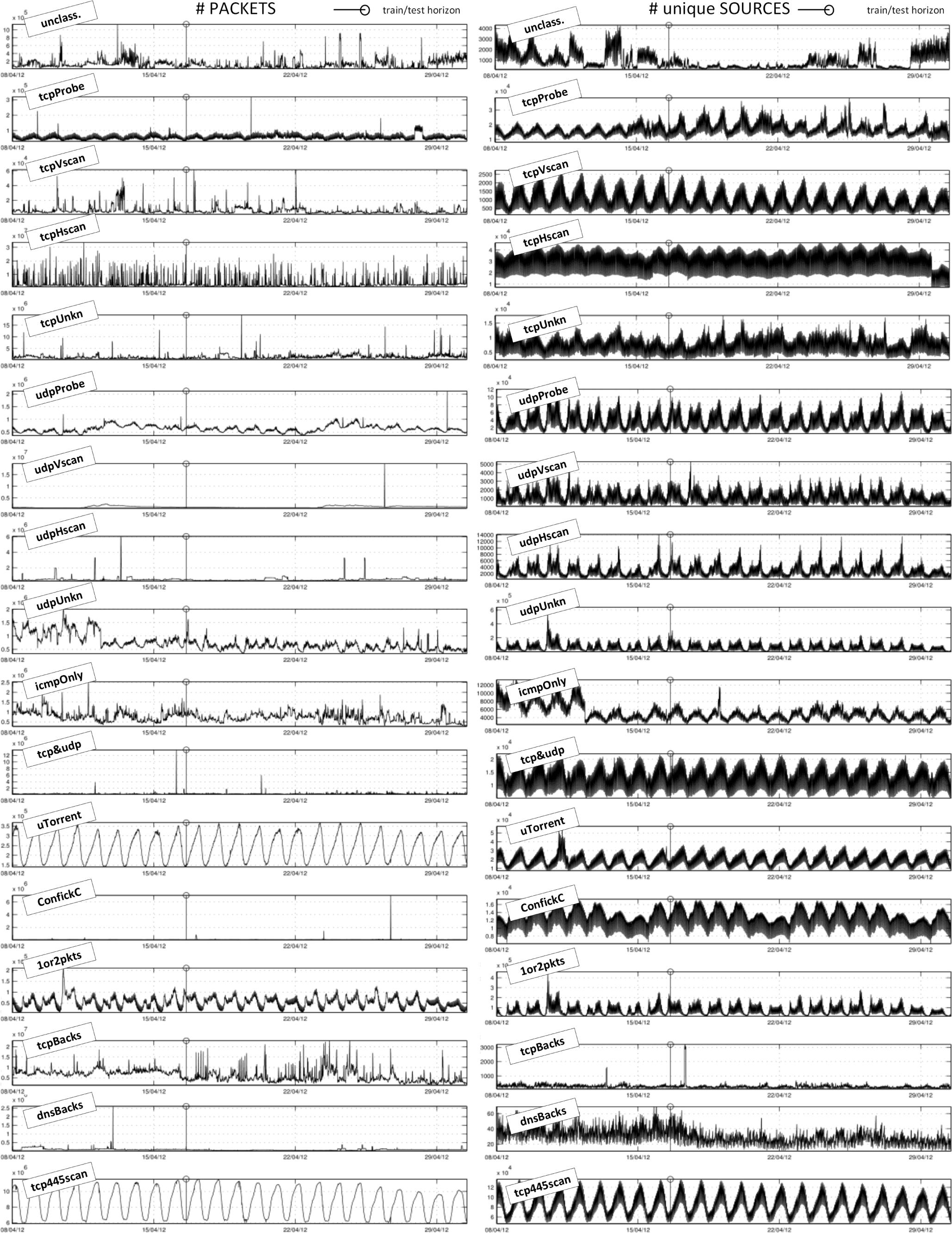
• Strong periodicity in sources: As a general rule, the amount of sources exhibits strong oscillations with an hourly rate. Furthermore, daily patterns are clearly visible in almost all cases, but for the dnsBacks, tcpBacks and unclass traffic sources.
• Dominant traffic in the IBR: Most of the packets observed in the darkspace belong to TCP horizontal scan activities; 35.2% are scans to port 445 (tcp445scan) and 14.2% are other TCP scan packets (tcpHscan). The huge amount of scan packets to port 445 is in line with observations made by others in different darkspaces (e.g., [9,28]). The scans correspond to vulnerabilities exploited by different worms and dramatically increased with the outbreak of the conficker worm in November, 2008 [12]. 28.6% of the traffic in the darkspace originates from responses to TCP scans with spoofed addresses (tcpBacks). As for the source types, sources scanning port 445 (tcp445scan), sources sending only one or two packets (1or2pkts) and sources sending UDP unknown traffic (udpUnk) stand for 57.5% of the active sources (within a 10-minute time scope).
• Rare correlation between packets and sources: With a few exceptions (see the next paragraph), the shapes of unique sources’ time series do not correlate with their respective packets time series, which show a much more irregular behavior. From a global perspective, we are observing an underlying periodic traffic that belongs to the majority of the active sources. Peaks in packets do not usually affect the shape of unique sources because such irregularities are caused by a few very active sources, i.e., strong packet peaks are caused by a few sources. Table 2, row “pkts/src”, shows the values of standard deviations very similar to or even higher than the mean values. Therefore, considering one traffic type, it denotes either frequent strong peaks in the packet time series or very different levels of activity in the sources over time.
  The few traffic types that show a correlation between packets and sources are 1or2pkts, uTorrent, and tcp445scan. For the 1or2pkts traffic class, the relationship between packets and sources is established by definition, because one source in this class sends either one or two packets. For the tcp445scan, it can be assumed that scan tools also send a more or less fixed number of packets per time interval. For the uTorrent traffic, the origin of the relation remains unclear. The traffic may originate from misconfiguration at a few senders, which probably send a fixed number of packets.
• The Patch Tuesday effect: The early peak in 1or2pkts packets and sources (April 11, 2012, 01:00 UCT) corresponds to Microsoft’s Patch Tuesday release. The Patch Tuesday effect in darkspace data has been described in [15]. The increment of suspicious activity for this date is also clearly noticeable in the amount of udpUnkn sources. It also generates noticeable peaks in tcpVscan, tcpUnk, udpUnkn, udpProbe, icmpOnly and unclass packets.
• Independence among packets, correlation among sources: The generalized strong hourly and daily cyclic behavior for the sources makes source types show a high correlation among each other, but for the dnsBacks, tcpBacks and unclass cases. As for the packet types, only uTorrent and tcp445scan (and tcpProbe to a minor degree) show correlated signals. Correlations among the remaining packet time series hardly overcome random relationships.
• Independent peaks: Peaks among packet types are usually not coincident, except for the Patch Tuesday case. The same is valid for source types if we consider peaks that are not expected as part of the daily cycles.

4. Entropy Analysis of Network Traffic

4.1. Obtaining Entropy Signals

In order to model the darkspace traffic, entropy metrics were applied to eight flow features obtained from the same pcap files that were deeply inspected in Section 3. The selected traffic-flow features are: IP source (srcIP), IP destination (dstIP), source port (srcPort), destination ports (dstPort), protocol (prot), flags (flag), time-to-live (TTL) and packet length (len). It is important to notice that entropy signals are calculated just based on the analysis of the feature distributions of the whole traffic. No pre-processing or classification of sources or packets into different traffic classes or origin-destination flows is necessary.

We use entropy as a compact metric to measure dispersion or concentration in a feature distribution. Since we work with real feature distributions and frequencies instead of probabilities, we use an entropy estimation, called sample entropy in [6], which is calculated as follows:

$$H(X)=-{\displaystyle \sum \left(\frac{n_i}{S}\right){\log }_2\left(\frac{n_i}{S}\right)}$$

(1)

H(X) stands for the entropy of the empirical histogram X. X represents a phenomenon (in our case, a traffic-flow feature) that can show N different states: 1…i…N, so n_i denotes the number of occurrences of the state i during the considered time interval for the sample. S = ∑ n_i.

The measure can be clearly understood with an example. The entropy of a histogram of active IP sources sending packets during a time interval of 10 min can be written as: H(srcIP)|_10′. In the case that only one source is active, we get only one peak in the histogram and get the minimum entropy: H(srcIP)|_10′ = 0. On the other hand, if all N sources send the same amount of packets during the interval, the histogram is fully dispersed, and we get the maximum entropy: H(srcIP)|₁₀ = log₂ N.

Entropy time series are obtained following the process scheme outlined in Figure 3. A MATLAB script is used to calculate entropy measures. Previously, data are pre-processed by corsaro: transformed from pcap to FlowTuple vectors and later aggregated to measure the occurrences every 10 min (the data aggregation is carried out with the cors_ft_aggregate tool, also from the corsaro suite). The FlowTuple format is displayed in Listing 2. Figure 4 displays the entropy time series for the analyzed traffic from April 8, 2012, 12:00 UTC, to May 1, 2012, 00:00 UTC.

Listing 2:. Corsaro FlowTuple Format

Listing 2:. Corsaro FlowTuple Format

<value> shows the number of packets in the pcap file whose header matches the given FlowTuple key. The FlowTuple key consists of source and destination IP addresses, source and destination port numbers, protocol type (usually TCP, UDP or ICMP), time-to-live (TTL) of the packet in the network, TCP flags (e.g., SYN, ACK, RST, used in TCP packets) and the length of the packet as specified in the packet header (details on FlowTuple format are at http://www.caida.org/tools/measurement/corsaro/docs/formats.html).

4.2. Univariate Analysis of Entropy Signals

The entropy signals from the different traffic features are shown in Figure 4. Entropy signals are studied in order to have a better understanding of the evolution of network flow feature distributions over time. Statistical information about the entropy time series is collected in

Table 3. Statistical data of entropy signals.

	H(srcIP)	H(dstIP)	H(srcPort)	H(dstPort)	H(prot)	H(flag)	H(TTL)	H(len)
Mean	11.82	21.14	10.26	7.28	0.83	5.03	1.54	2.94
SD	1.37	0.67	1.25	1.26	0.11	0.25	0.16	0.24
daily per.	first	second	second	second	first	—	second	first
weekly per.	—	first	first	first	—	—	first	—
Distribution
	negatively skewed	close to normal, strong neg. outliers	Close to normal, positively skewed	close to normal, short tails, slightly neg. skewed	Close to normal, positively skewed	positively skewed	strong pos. outliers	strong pos. outliers
Peaks*	weak	strong	weak	weak	weak	weak	strong	strong
main	2658 (−)	2654 (−)	509 (−)	2231 (+)	1344 (−)	1218 (−)	2698 (+)	2654 (+)
Second	2956 (−)	2655 (−)	2658 (−)	2654 (+)	509 (−)	1634 (−)	2697 (+)	2655 (+)
Third	509 (−)	—	2219 (−)	2261 (+)	542 (+)	2956 (−)	2221 (+)	1837 (+)

per.: periodicity; pos.: positive; neg.: negative; (−): local/global minimum; (+): local/global maximum;

^*values correspond to sample IDs (timely ordered). Every sample covers 10 min of analyzed traffic.

. The correlation matrix for the entropy signals from different features is provided in

Table 4. Correlation matrix of entropy signals.

	H(srcIP)	H(dstIP)	H(srcPort)	H(dstPort)	H(prot)	H(flag)	H(TTL)	H(len)
H(srcIP)	1	−0.61	0.91	−0.21	0.57	0.64	0.20	0.38
H(dstIP)	−0.61	1	−0.66	0.05	−0.71	−0.64	−0.38	−0.65
H(srcPort)	0.91	−0.66	1	−0.35	0.56	0.67	0.10	0.39
H(dstPort)	−0.21	0.05	−0.35	1	0.09	0.07	0.67	0.26
H(prot)	0.57	−0.71	0.56	0.09	1	0.61	0.44	0.73
H(flag)	0.64	−0.64	0.67	0.07	0.61	1	0.40	0.57
H(TTL)	0.20	−0.38	0.10	0.67	0.44	0.40	1	0.49
H(len)	0.38	−0.65	0.39	0.26	0.73	0.57	0.49	1

. A close look at Figure 4 and Tables 3 and 4 reveals some interesting aspects to underline:

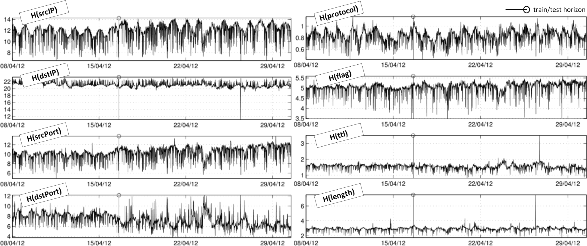
• Daily and weekly trends in traffic: Variations in the distribution of the studied signals follow daily and weekly trends for all features, except for the flag feature. In other words, there are network phenomena submitted to daily and weekly recurrence patterns whose activity does not involve a characteristic effect on the flag values of their packets, but actually affects the rest of analyzed features. The distribution of IP sources, protocols and packet lengths exhibit a daily pattern. IP destination, source port and destination port distributions additionally show weekly repetitions.
• Nature of entropy distributions, skewed or disrupted by strong peaks: We also looked at the distribution of the entropy values (each value calculated from a 10-minute time interval) for the different features in order to see how the entropy values taken at different time intervals vary. Distributions of H(srcIP), H(TTL) and H(len) are far from being normal and skewed to more concentrated performances (source IPs) or dispersed states (TTLs and lengths). The intrinsic characteristics of every feature must be taken into account, i.e., IP sources are categorical values and their variability is much higher than possible values taken by TTLs and packet lengths. Furthermore, a few strong sources that suddenly become active can lead to a concentration of the srcIP feature distribution and can cause a sudden decrease in the entropy. In contrast, the entropy of destIP is always quite high, because sources target many different destinations if they scan the address space or answer to spoofed addresses. Protocols, source and destination port entropy distributions are closer to normal, but also skewed. The distribution of destination IP entropy is quite close to normal, but it is seriously disrupted by an isolated negative peak (outlier) that happens on April 26 at 22:30 UTC (corresponding to a udpVscan peak). The peak is clearly visible in Figure 4, H(dstIP) plot.
• Strong common peaks: Destination IP, TTL and packet length entropies exhibit strong peaks compared to their normal values. The most significant peak on April 26, 2012, at 22:30 UTC is noticeable in all entropy signals within a 30-minute scope, but for the TTL case (the closest strong peak of H(TTL) happens five hours later, and it is related to a different event: ConfickC peak). This peak around April 26 is especially significant in the following entropy signals: IP sources, IP destinations, source ports, destination ports and packet lengths. The coincidences of peaks among entropy signals happen frequently.
• Entropies are directly correlated, but for the IP destination entropy, which shows an inverse correlation: All signals under test show some positive correlations among them, but for the case of the IP destination entropy, which presents an inverse correlation to the other time series (except of the destination port entropy). Especially high are the positive correlations between IP source and source port entropies, also between flags and protocols, as well as the inverse correlation between IP destinations and protocols (some of theses correlation have been previously documented in [8]). The strong correlation between IP source and the source port is probably caused by the fact that sources select a random source port when sending an unsolicited packet. Therefore, if new sources become active, also new source ports are used. On the other hand, the negative correlation between the IP destination entropy and other feature entropies manifests that the increase of different target destinations mainly corresponds to automated algorithms sending clonal packets (e.g., scans); hence, the variability of other features decreases, since only the IP destination (sometimes also the destination port) are different. Finally, the destination port entropy shows quite random relationships with most of the other distributions, but for the TTL case.

5. Entropy-Based Modeling of the IP Darkspace

In this section, we describe how traffic types obtained by deep analysis inspection were modeled by using entropy signals. We use entropy signals from all features as input and try to derive a model for a specific smee class. We repeat this for all smee traffic classes. The goal is to be able to deduce changes in a specific smee traffic class simply by looking at the entropy signals without any deep packet inspection. We also provide information about the used methodologies and parameterization.

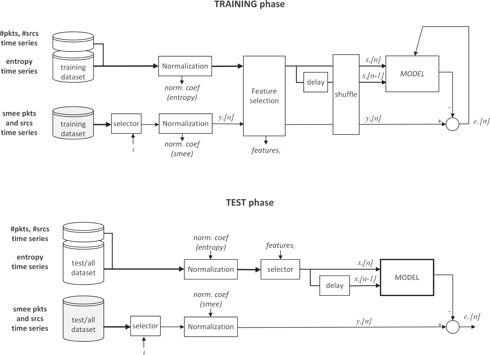
5.1. Modeling Scheme

Experiments covered two different phases: training, where models were tuned by means of supervised learning algorithms; and test, where models were checked with data not used during the training phase. There was actually a second test phase, where test experiments were repeated using together the test and training datasets. In Figure 5, both processes are carefully depicted. The description of blocks and signals in the figure is provided as follows:

• Datasets.

  • Entropy time series, i.e., signals corresponding to distribution measures of flow-traffic features. We introduced them in Section 4, and they are displayed in Figure 4.
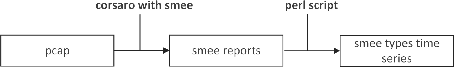
  • Smee time series of sources and packets, introduced in Section 3 and shown in Figure 1.
  • Total amount of packets (#pkts) and total amount of sources (#srcs), considering the whole darkspace and collected every 10 min. These two signals are easy to obtain and do not require any in-depth analysis.
  The introduced datasets were split according to the deployment for the training and test phases. Training: 2000 samples, from April 8, 2012, 12:00 UTS, to April 17, 2012, 2:40 UTC); test: 1240 samples, from April 17, 2012, 2:50 UTC, to May 1, 2012, 00:00 UTC.
• Selectors, applied in two different contexts:

  • To filter the specific smee type time series to the model. i ∈ [1, …, 34] identifies every one of the time series displayed in Figure 1.
  • To filter the set of entropy features required to feed the model. The specific group of features for every modeled smee (i.e., features_i) depends on the feature selection process carried out during the training phase.
• Normalization was performed for all signals by using z-score transformations (statistical normalization); therefore, every time series got $\overline{x}=0$ and σ² = 1. Since, in a real case, test data would be captured on-line and therefore unknown during the model tuning phase, normalization coefficients found during the training phase were also utilized later to normalize test data.
  We additionally performed an ad hoc normalization (s-normalization) for displaying some results and figures in Section 6. This s-normalization is a linear manipulation of the x̄ and σ² in order to fit more friendly rates for the implementation of a monitoring system prototype. Here, values “5” and “15” respectively stand for the signal under the test minimum and maximum during training data.
• Feature selection was carried out during the training phase by using least angle regression (LARS) with the least absolute selection and shrinkage operator (LASSO). This method is described in the next subsection, Section 5.2.
• The shuffle block jumbled input samples before presenting the vectors to the models during the training phase in order to avoid overfitting. The new set of samples is reordered by a pseudorandom number generator given a prefixed random seed.
• A delay step was applied to the inputs, doubling the number of predictors. Hence, models were also optionally provided with memory capabilities (entropy derivatives) to fit traffic types, i.e., the model additionally deployed x[n − 1] and not only x[n] as part of the input vector.
• Model. This block contains the regression algorithm deployed for modeling smee type time series. The different modeling methodologies tested in this work are described in the next subsection, Section 5.2. During the training phase, model outputs were compared to real values of the signal to abstract in order to tune the model with the obtained error. In the test phase, the error is stored to evaluate model performances.

5.2. Regression Techniques

We opted to use various regression techniques and to evaluate their capabilities and limitations to model traffic types. We aimed to shed light on two main questions:

• Is there any direct dependence between traffic types and flow-traffic feature entropies? If so, can we describe the relationships between them for specific traffic types?
• Is it possible to create entropy-based models for the indirect prediction of the traffic types amount?

The utilized regression models are as follows:

• Least angle regression with LASSO:
  The LAR/LASSO solution performs linear regression, as well as evaluates the contribution of every input feature by providing a coefficient vector β, which expresses feature relevancy. In this work, we mainly used this method for feature selection, yet its linear regression performances were also considered in comparison with the rest of the models. The undertaken implementation is based on the algorithm proposed by Efron et al. in [29].
  For every studied smee type, the LASSO threshold was fixed after a combination of linear and logarithmic parameter optimization. All of the subsequent models were run twice: fed with all features and only with the feature set recommended by the LASSO.
• Artificial neural network (ANN):
  ANNs have been widely applied to solve classification and regression problems submitted to strong non-linearities and chaotic behaviors. An ANN emulates biological neural networks by presenting a highly parallel architecture to process input vectors. Here, we developed a classic feed-forward multi-layer perceptron, which was trained with a back propagation algorithm [30]. The network hidden layer size was (#features + #classes)/2 + 1; the training cycles were 1000, the learning rate 0.25 and the momentum 0.05, and the optimization was stopped when the error rate dropped below 1.0 × 10⁻⁵.
• k-nearest neighbor classifier (kNN)
  A kNN regression model consists of a simple nonparametric algorithm, which elaborates a problem map with the training samples and predicts the numerical target of a test sample by weighting the responses of the most similar training cases (neighbors) [31]. For the experiments, the distance metric was Euclidean-based, k was set to five neighbors and the contribution of every neighbor was proportionally weighted according to the distance to the test sample.
• Gaussian process (GP):
  A Gaussian process is quite a generally valid non-parametric technique for regression and prediction. In Gaussian processes, it is assumed that input data can be represented as a sample from a multivariate Gaussian distribution. Gaussian processes are more subtle than other fitting techniques, as they parameterize the data covariance structure instead of any regression function [32]. For the experiments, the used kernel type was a radial basis function (rbf), the kernel length-scale was set to 3.0, the maximum number of basis vectors to be used was 100 and the epsilon and geometrical tolerances were both set to 1.0 × 10⁻⁷.
• Polynomial regression:
  In a polynomial regression, data are forced to fit an n order polynomial function. Given a signal to model (y_r), for the case with one independent variable (x) and one dependent variable or predicted outcome (y_p), y_p can be expressed as follows:

  $$y_p=a_0+a_1\times x+a_2\times x^2+\dots +a_n\times x^n$$

  (2)

  where a₀, …, a_n are the coefficients of the polynomial. Function coefficients are adjusted by using the least squares method: e = y_r − y_p(x); e stands for error.
  Polynomial regression is one of the simplest linear regression models; we utilized it to find linear correlations whenever possible, as they are the simplest and most understandable expressions of causal relationships. For the experiments, the maximum number of iterations was set to 5000, and the maximum degree of the polynomial was five.

6. Results

Considering together the blocks and models introduced in Sections 5.1 and 5.2, some figures about the total number of compared evaluations can be calculated. Every smee type (17 types) has been analyzed, dealing separately with sources and packets (two variables). All available entropy features, as well as only the subset obtained after feature selection were tested (two subsets). Predictors took values for the same time period, but additionally, the previous 10-minute slot was considered (two time configurations). Diverse regression models were utilized in every test (five models). Finally, every single experiment underwent a training phase, and two test phases (only test data and test + training data together). Therefore, without taking into account the parameter optimization carried out for the feature selection and the model tuning, for every of the 34 analyzed signals (17 types × 2 variables = 34), 20 training and 40 test performance values were obtained and compared.

Table 5. Smee signals than can be predicted by means of entropy measures.

Smee case	pkts/srcs	entropy - H(…)	other	best model	yt = …	RMSE*
1or2pkts	pkts	prot	#srcs	ANN	f(xt, xt−1)	0.26 (test) 0.20 (all)
tcp445scan	pkts	srcIP, dstPort, prot	#pkts,	ANN	f(xt, xt−1)	0.44 (test) 0.36 (all)
tcpBacks	pkts	dstIP, srcPort, dstPort, prot, flags,	#pkts,	ANN	f(xt)	0.77 (test) 0.63 (all)
tcpHscan	pkts	srcIP, dstIP, dstPort, TTL	#pkts	GP	f(xt)	0.35 (test) 0.30 (all)
udpVscan	pkts	srcIP, dstIP len	#pkts #srcs	LARS/LASSO	f(xt)	0.92 (test) 0.79 (all)
uTorrent	pkts	srcIP, dstIP, dstPort, prot, flag	#pkts #srcs	ANN	f(xt)	0.45 (test) 0.40 (all)
1or2pkts	srcs	srcIP, dstIP, prot, TTL	#pkts #srcs	ANN	f(xt, xt−1)	0.21 (test) 0.19 (all)
tcp445scan	srcs	srcIP, dstPort, prot	#pkts, #srcs	ANN	f(xt, xt−1)	0.43 (test) 0.37 (all)
udpHscan	srcs	prot, TTL	#srcs	LARS/LASSO	f(xt)	0.48 (test) 0.48 (all)
udpVscan	srcs	srcIP, prot	#pkts #srcs	LARS/LASSO	f(xt)	0.31 (test) 0.32 (all)
udpProbe	srcs	srcIP, dstIP, dstPort, prot, TTL	#srcs	ANN	f(xt)	0.26 (test) 0.25 (all)
udpUnk	srcs	srcIP, srcPort, dstPort, prot,	#pkts #srcs	ANN	f(xt, xt−1)	0.17 (test) 0.15 (all)
tcp&udp	srcs	srcIP, srcPort, dstPort, prot, TTL	#pkts #srcs	ANN	f(xt, xt−1)	0.34 (test) 0.23 (all)
uTorrent	srcs	srcIP, dstIP, dstPort, prot	#pkts #srcs	ANN	f(xt, xt−1)	0.43 (test) 0.44 (all)

^*calculated from s-normalized signals.

displays information about the signals that can be predicted by using entropy values. Given a traffic type, the entropy row shows the features whose entropy had a meaningful contribution for the best performance in the respective set of experiments. Similarly, the other row refers to non-entropy inputs, which contributed to the best prediction. The best model row shows the model that obtained the lowest error rate (i.e., the lower root-mean-square deviation or RMSE). Supplied RMSE values correspond to s-normalized signals. On the other hand, the y = … row informs us if the model required delayed or not delayed values of the entropy signals to achieve a better performance.

To summarize the results, qualitative assessments are provided in

Table 6. Smee signals liable to be predicted by entropy-based models.

	unclass.	tcpProb	tcpVscan	tcpHscan	tcpUnk	udpProb	udpVscan	udpHscan	udpUnk
PACKETS	—	—	—	good	—	—	good	—	—
SOURCES	—	—	—	—	—	good	poor	acceptable	excellent
	icmpOnly	tcp&udp	uTorrent	concfickC	1 or 2	tcpBacks	dnsBacks	tcp445scan
PACKETS	poor	—	acceptable	—	excellent	good	—	good	—
SOURCES	—	good	acceptable	—	excellent	—	—	good	—

, which was elaborated after comparing error indices, as well as inspecting how the original time series matched the predicted ones. Figures 6, 7 and 8 display the subset of predictable time series, comparing the original and the predicted signals, as well as showing the corresponding obtained error for each case (values of the y-axes are s-normalized). Finally,

Table 7. Smee types predictable by polynomial regression.

Smee case	linear terms	quadratic terms	cubic terms
tcpHoritz (pkts)	−a1H(srcIP), +b1H(dstIP), −d1H(dstPort), −f1H(TTL), +m1#pkts
udpVscan (pkts)	−a1H(srcIP), +b1H(dstIP), −h1H(len), +m1#pkts, −n1#srcs
tcpBacks (pkts)	−b1H(dstIP), +c1H(srcPort), +d1H(dstPort), −e1H(prot), −g1H(flags), +m1#pkts
udpProbe (srcs)	−a1H(srcIP), −b1H(dstIP), +d1H(dstPort) −f1H(TTL), +n1#srcs		+e3H(prot)3
*udpVscan (srcs)	−a1H(srcIP), −g1H(flags), −m1#pkts, +n1#srcs	+e2H(prot)2
*udpHscan (srcs)	+e1H(prot), +n1#srcs	+f2H(TTL)2
udpUnk (srcs)	−a1H(srcIP), −c1H(srcPort), +d1H(dstPort), +e1H(prot), −m1#pkts, +n1#srcs
1or2pkts (srcs)	−a1H(srcIP), +e1H(prot), −f1H(TTL), −m1#pkts, +n1#srcs	+b2H(dstIP)2
tcp445Hscan (srcs)	a1H(srcIP), −d1H(dstPort), −e1H(prot), +m1#pkts, +n1#srcs

^*Problems to match strong peaks.

displays the traffic type signals that can be satisfactorily modeled using polynomial regression techniques.

7. Discussion

Experiment results show that some network anomalies can be traced by looking at the imprint they leave on the distribution of flow-traffic features. Assuming a certain normality in the proportion of traffic types (in a wide sense), they can even be accurately predicted by regression models. Periodic feedback with the results of deep inspection techniques allows the adjustment of models to fit new network traffic normality. Furthermore, results reveal the following findings:

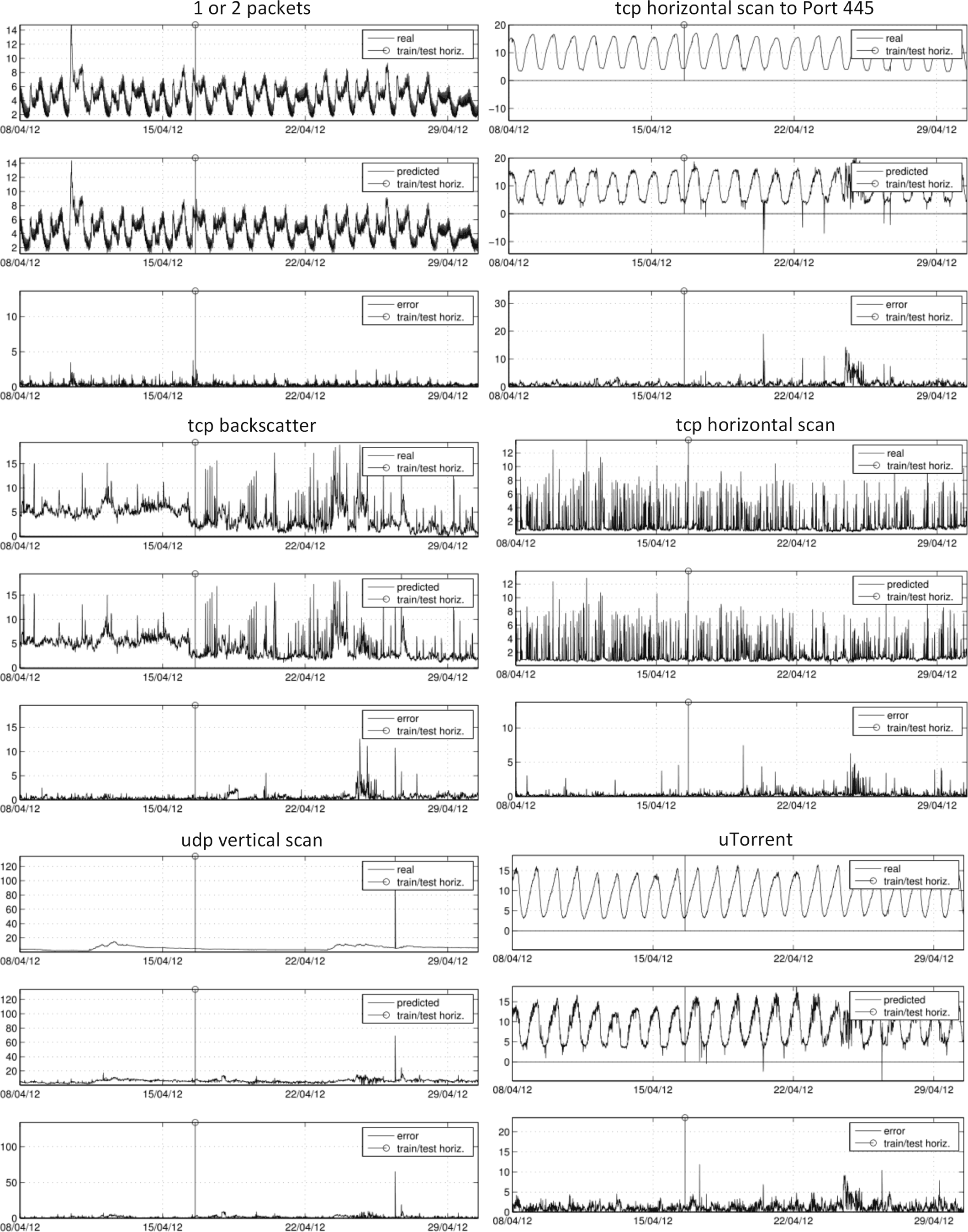
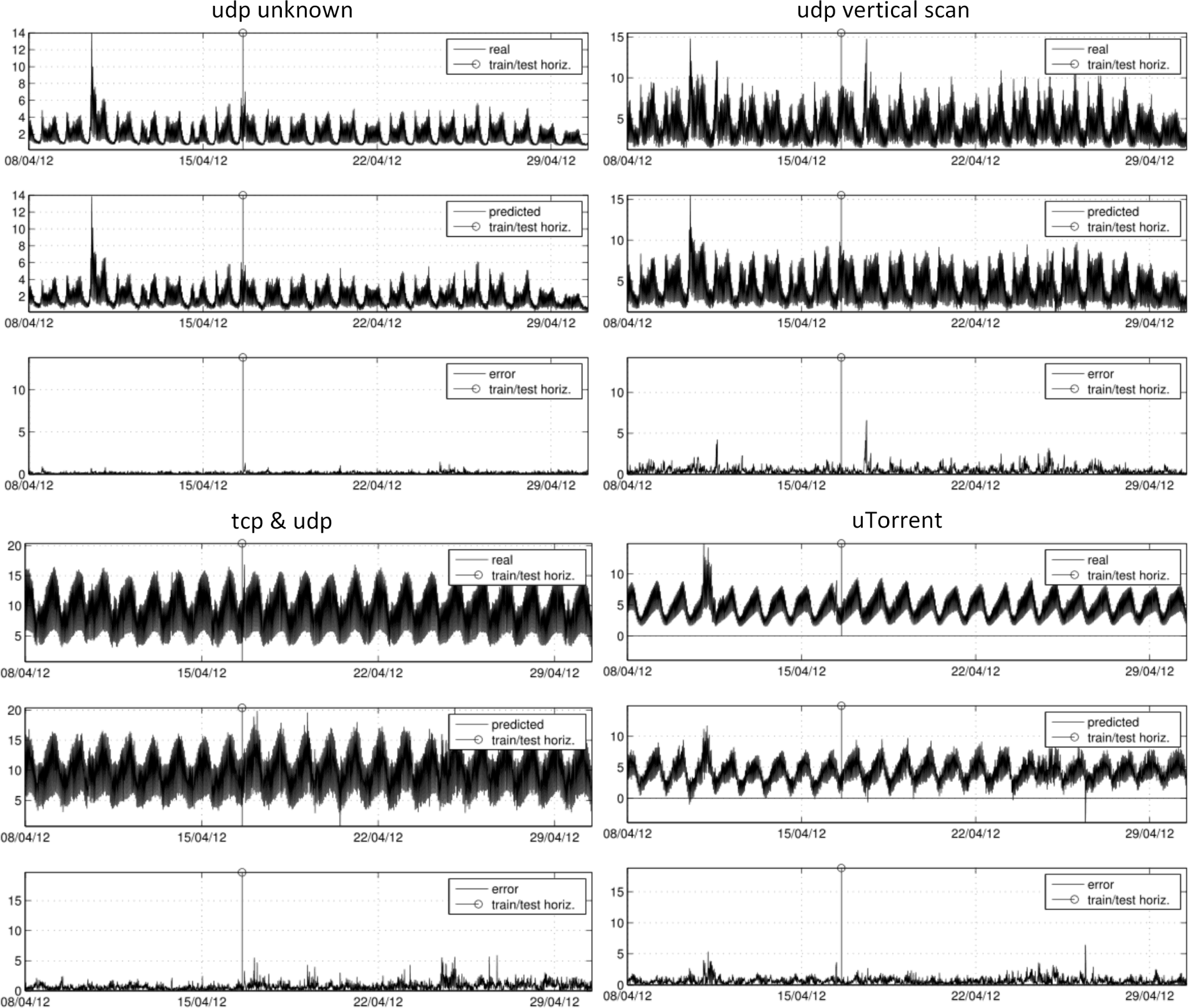
• Predictable packet types: Six out of 17 packet types can be satisfactorily modeled with an acceptable error rate. Predictable types coincide with the types that cover the highest percentage of the total traffic, e.g., tcpBacks (25.3%), tcp445scan (35.2%) tcpHscan (14.2%) and udpVscan (4.7%), which shares the fourth rank with a more irregular and unpredictable tcpUnk traffic. Such results are expected, as they significantly contribute to shape entropy signals. The contribution of other types with a lower presence can hardly be detected, partially because they are masked by noisy traffic and the more dominate traffic types or because they do not leave a significant imprint in the distribution of traffic-flow features. Exceptions are 1or2 (0.2%) and uTorrent (%1.0), whose particular and stable profiles make them traceable, even in spite of their low presence.
• Peak of udpVscan (packets): The peak on April 26 at 22:30 UTC, which relates to a sudden vertical scan on a specific machine, can be directly tracked in most of the entropy signals, most significantly for H(dstIP), H(dstPort) and H(length).
• Peak of ConfickC (packets): The peak on April 27 at 05:40 UTC, which relates to an increase of Conficker.C traffic, can be directly tracked in H(TTL). Regression models were not able to capture this evident correlation, because there was not any ConfickC peak in the training data.
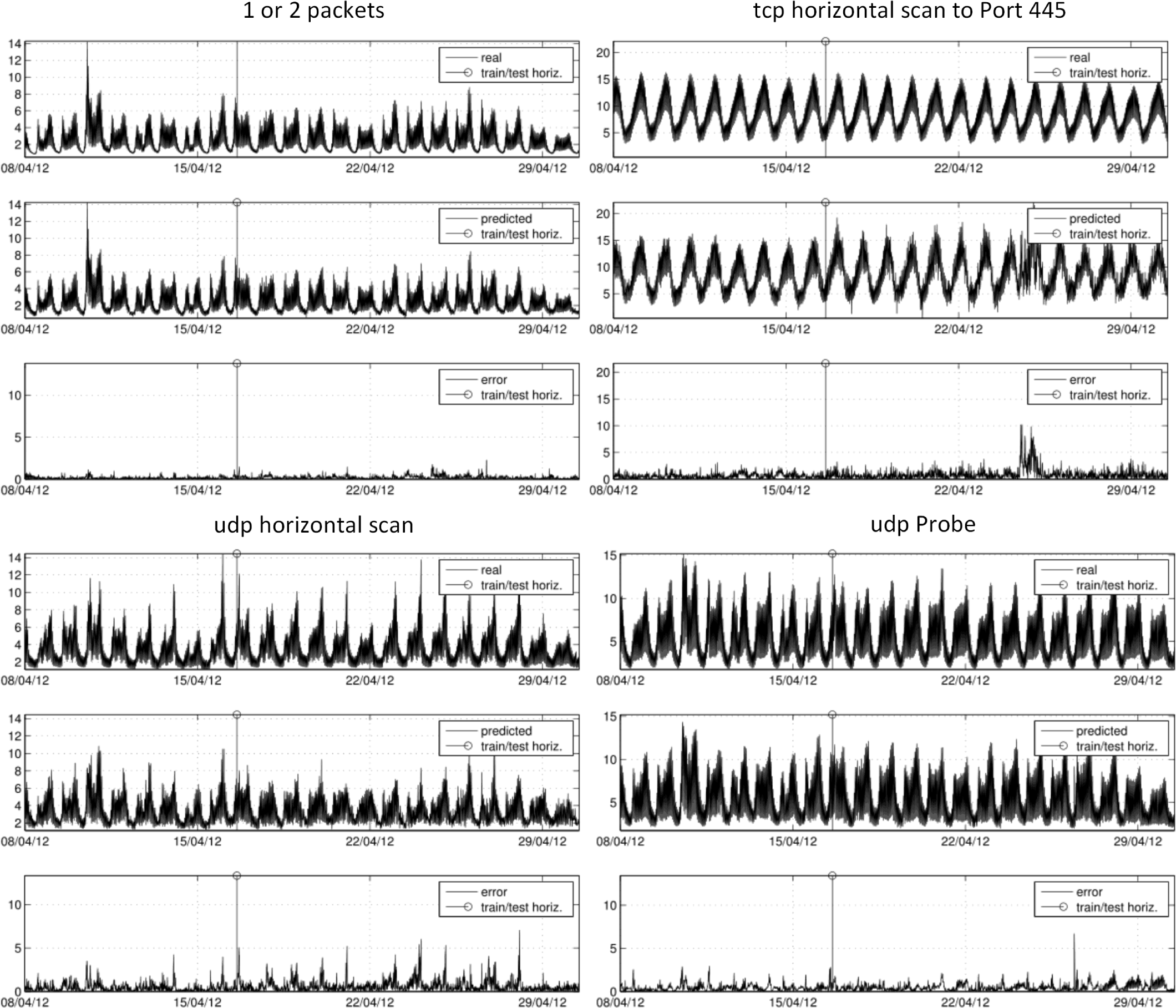
• Predictable source types: To expect that the most common source types also contribute the most to the entropy signals could be misleading, as entropy signals are calculated from traffic packets as samples and not source types. In any case, there is an obvious correlation, and the four most common sources are traceable in our experiments (percentage values correspond to means obtained with a 10-minute time scope): tcp445scan (26.1%), 1or2 (16.6%), udpUnk (14.8%) and udpProb (9.6%). Although they have a lesser contribution, udpVscan, udpHscan, tcp&udp and uTorrent can be also satisfactorily modeled. The strong periodical (hourly, half-day and daily) behavior of source types is an advantage for regression methods in order to fit the general tendencies, but at the same time, it is a drawback that leads to overfitting and makes models unable to adequately match spontaneous peaks or events that break normal trends. This is noticeable in the difficulties in achieving some peaks in some cases, e.g., udpHscan or udpVscan.
• Unstable period of predictions: There is a disruption in some of the predicted signals from Samples 2370 to 2520 (approximately, from Tuesday, April 24, 2012, 23:00:00, to Thursday April 26, 2012, 00:00:00; 25 h). There is nothing significant, neither in entropy signals nor in smee types, that justifies this disrupted span. Means and standard deviations of packets and sources during this time period do not significantly differ from the statistics for the whole time series. Therefore, some phenomena may remain undetected, even with deep packet inspection analysis.
• Interpretation of dependencies and correlations: Bringing together all of the conducted analyses, we can roughly conclude that we found a correlation among entropy signals, a correlation among types of traffic sources and a lack of correlation among types of traffic packets. In a similar way, we found coincident peaks in entropies and sources, and non-coincident peaks in packets. Such behaviors indicate a stable, easily predictable traffic mass with strong hourly and daily periodicities that accounts for the majority of sources and a considerable rate of packets. Anomalies of this normality in the darkspace are not due to the massive arrangement of sources, but to a few sources with a sudden high activity. As we have seen in the predicted signals, this sudden high activity (peaks in packet types) can be detected by indirect measures of entropy over traffic flow features, at least in those traffic types that define a significant part of the traffic when considering the whole time scope.

8. Conclusions

In this work, the deep analysis of traffic from a large/8 IP darkspace captured during three weeks of April, 2012, is compared to a more lightweight traffic characterization method that is solely based on the entropy signals of different traffic features. The deep analysis disclosed a recent picture of the IBR, reflecting trends of network attacks and anomalies on a large scale with dominant traffic characterized by TCP scanning activities (mostly to port 445) and TCP backscatter. Furthermore, whereas rates of distinct traffic-type sources show a strong, stable periodical behavior (with clear hourly, half-day and daily trends), from the global perspective, the traffic itself (packets) is actually chaotic, hardly periodical and unexpected. This means that the IBR is formed by an underlying, stable traffic wave, where anomalies (strong peaks and disruptions) are concentrated on the activity of few sources.

Our analysis shows that anomalies that belong to variations of representative (non-rare) traffic types can be predicted by entropy-based models very well. Indeed, the most common traffic types (for both packets and sources) can be traced, modeled and predicted by using entropy measures of traffic flow features. This fact introduces future improvements for network monitors in charge of wide network areas, whose context awareness capabilities are accelerated and upgraded by adding lightweight entropy-based analysis. Such enhancements still require a periodical support provided by occasional deep inspection analysis in order to fit the continuously evolving network normality, yet they do not have to run in the forefront of the detection and can operate over reduced portions of traffic and with lower time restrictions. With this, entropy-based methods can be a valuable building block for early warning systems and the detection of new attacks and attack preparation activities.

References

- Floyd, S.; Paxson, V. Difficulties in Simulating the Internet. IEEE/ACM Trans. Netw. 2001, 9, 392–403. [Google Scholar]
- Dainotti, A.; Pescape, A.; Claffy, K. Issues and future directions in traffic classification. IEEE Netw. 2012, 26, 35–40. [Google Scholar]
- Paxson, V. Bro intrusion detection system 2009. Available online: http://www.bro-ids.org accessed on 15 December 2014.
- PACE 2.0, Protocol and Application Classification with Metadata Extraction 2014. Available online: http://www.ipoque.com/en/products/pace accessed on 15 December 2014.
- CISCO. Network-Based Application Recognition, 2007, Classifying Network Traffic Using NBAR. Available online: http://www.cisco.com/c/en/us/td/docs/ios/12_4t/qos/configuration/guide/qsnbar1.html accessed on 15 December 2014.
- Lakhina, A.; Crovella, M.; Diot, C. Mining anomalies using traffic feature distributions. SIGCOMM Comput. Commun. Rev. 2005, 35, 217–228. [Google Scholar]
- Tellenbach, B.; Burkhart, M.; Sornette, D.; Maillart, T. Beyond Shannon: Characterizing Internet Traffic with Generalized Entropy Metrics. In Passive and Active Network Measurement, Proceedings of the 10th International Conference, PAM 2009, Seoul, Korea, 1–3 April 2009; Moon, S.B., Teixeira, R., Uhlig, S., Eds.; Springer: Berlin/Heidelberg, Germany, 2009; pp. 239–248. [Google Scholar]
- Zseby, T.; Brownlee, N.; King, A.; Claffy, K. Nightlights: Entropy-based Metrics for Classifying Darkspace Traffic Patterns. In Passive and Active Measurement, Proceedings of the 15th International Conference, PAM 2014, Los Angeles, CA, USA, 10–11 March 2014; Faloutsos, M., Kuzmanovic, A., Eds.; Springer: Berlin/Heidelberg, Germany, 2014; pp. 275–277. [Google Scholar]
- Wustrow, E.; Karir, M.; Bailey, M.; Jahanian, F.; Huston, G. Internet Background Radiation revisited, Proceedings of The 2010 ACM Internet Measurement Conference, Melbourne, Australia, 1–30 November 2010; pp. 62–74.
- Moore, D.; Paxson, V.; Savage, S.; Shannon, C.; Staniford, S.; Weaver, N. Inside the Slammer Worm. IEEE Secur. Priv. 2003, 1, 33–39. [Google Scholar]
- Moore, D.; Shannon, C.; Brown, D.; Voelker, G.; Savage, S. Inferring Internet Denial-of-Service Activity. ACM Trans. Comput. Syst. 2006, 24, 115–139. [Google Scholar]
- Aben, E. Conficker/Conflicker/Downadup as seen from the UCSD Network Telescope. Available online: http://www.caida.org/research/security/ms08-067/conficker.xml accessed on 15 December 2014.
- Brownlee, N. One-way Traffic Monitoring with Iatmon. In Passive and Active Measurement, Proceedings of The 13th International Conference on Passive and Active Measurement (PAM 2012), Vienna, Austria, 12–14 March 2012; Taft, N., Ricciato, F., Eds.; Springer: Berlin/Heidelberg, Germany, 2012; pp. 179–188. [Google Scholar]
- Dainotti, A.; King, A.; Claffy, K.; Papale, F.; Pescape, A. Analysis of a “/0” Stealth Scan from a Botnet, Proceedings of the 2012 ACM Conference on Internet Measurement Conference, Boston, MA, USA, 14–16 November 2012; pp. 1–14.
- Zseby, T.; King, A.; Brownlee, N.; Claffy, K. The Day After Patch Tuesday: Effects Observable in IP Darkspace Traffic, Proceedings of Passive and Active Network Measurement Workshop (PAM’13), Hong Kong, China, 18–19 March 2013; pp. 273–275.
- Dainotti, A.; Squarcella, C.; Aben, E.; Claffy, K.C.; Chiesa, M.; Russo, M.; Pescapé, A. Analysis of Country-wide Internet Outages Caused by Censorship, Proceedings of The 2011 ACM Internet Measurement Conference, Berlin, Germany, 2–4 November 2011; pp. 1–18.
- Zseby, T.; Claffy, K. Workshop Report: Darkspace and Unsolicited Traffic Analysis (DUST). SIGCOMM Comput. Commun. Rev. 2012, 42, 49–53. [Google Scholar]
- CAIDA. The CAIDA UCSD Network Telescope “Patch Tuesday” Dataset. Available online: http://www.caida.org/data/passive/telescope-patch-tuesday_dataset.xml accessed on 22 December 2014.
- Corsaro, version 2.1.0; software suite for performing large-scale analysis of trace data; CAIDA: La Jolla, CA, USA, 2014.
- Treurniet, J. A Network Activity Classification Schema and Its Application to Scan Detection. IEEE/ACM Trans. Netw. 2011, 19, 1396–1404. [Google Scholar]
- Kim, M.S.; Kong, H.J.; Hong, S.C.; Chung, S.H.; Hong, J. A flow-based method for abnormal network traffic detection, Proceedings of The 10th IEEE/IFIP Network Operations and Management Symposium (NOMS 2004), Seoul, Korea, 19–23 April 2004; 1, pp. 599–612.
- Ziviani, A.; Gomes, A.T.A.; Monsores, M.; Rodrigues, P. Network anomaly detection using nonextensive entropy. IEEE Commun. Lett. 2007, 11, 1034–1036. [Google Scholar]
- Gu, Y.; McCallum, A.; Towsley, D. Detecting Anomalies in Network Traffic Using Maximum Entropy Estimation, Proceedings of The 2005 ACM Internet Measurement Conference, New Orleans, LA, USA, 19–21 October 2005; pp. 32–32.
- Pang, R.; Yegneswaran, V.; Barford, P.; Paxson, V.; Peterson, L. Characteristics of Internet Background Radiation, Proceedings of The 2004 ACM Internet Measurement Conference, Taormina, Italy, 25–27 October 2004; pp. 27–40.
- Ahmed, E.; Clark, A.; Mohay, G. Effective Change Detection in Large Repositories of Unsolicited Traffic, Proceedings of The Fourth International Conference on Internet Monitoring and Protection (ICIMP’09), Venice, Italy, 24–28 May 2009; pp. 1–6.
- Iglesias, F.; Zseby, T. Modelling IP darkspace traffic by means of clustering techniques, Proceedings of 2014 IEEE Conference on Communications and Network Security (CNS), San Francisco, CA, USA, 29–31 October 2014; pp. 166–174.
- Porras, P.; Saidi, H.; Yegneswaran, V. Conficker C P2P Protocol and Implementation. Available online: http://mtc.sri.com/Conficker/P2P/ accessed on 22 December 2014.
- Bailey, M.; Cooke, E.; Jahanian, F.; Nazario, J.; Watson, D. The Internet Motion Sensor: A Distributed Blackhole Monitoring System, Proceedings of The 2005 Network and Distributed System Security Symposium (NDSS’05), San Diego, CA, USA, 2–4 February 2005; pp. 167–179.
- Efron, B.; Hastie, T.; Johnstone, I.; Tibshirani, R. Least angle regression. Ann. Stat. 2004, 32, 407–499. [Google Scholar]
- Riedmiller, M. Advanced supervised learning in multi-layer perceptrons: From backpropagation to adaptive learning algorithms. Comput. Stand. Interfaces 1994, 16, 265–278. [Google Scholar]
- Samworth, R.J. Optimal weighted nearest neighbour classifiers. Ann. Stat. 2012, 40, 2733–2763. [Google Scholar]
- Rasmussen, C.E.; Williams, C.K.I. Gaussian Processes for Machine Learning; Adaptive Computation and Machine Learning Series; The MIT Press: Cambridge, MA, USA, 2005. [Google Scholar]