
Modified Legendre Wavelets Technique for Fractional Oscillation Equations

Abstract
:1. Introduction
- (1)
- single-well
- (2)
- double-well
- (3)
- double-hump
2. Legendre Wavelets and Picard’s Iteration
2.1. Legendre Wavelets
Convergence
2.2. Picard’s Iteration
3. Applications

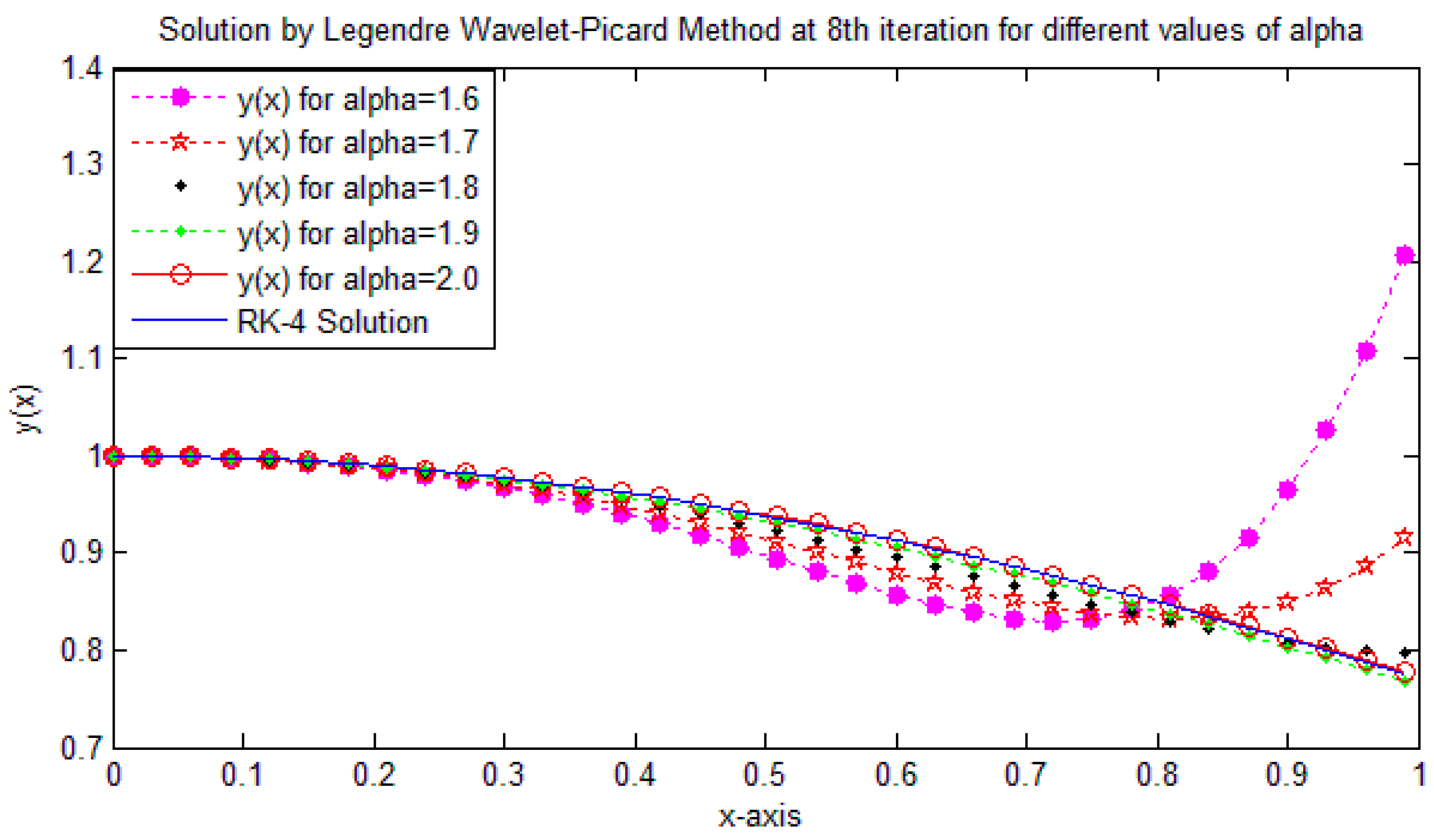
| t | VIM Solution | UWCM [24] Solution at M = 6 | LWPM Solution at M = 6 | RK-4 Solution | Error in UWCM [24] | Error in LWPM |
|---|---|---|---|---|---|---|
| 0.0 | 1.00000000 | 1.00000000 | 1.00000000 | 1.00000000 | 1.0 × 10⁻⁹ | 1.2 × 10⁻¹⁰ |
| 0.1 | 0.99750286 | 0.99750276 | 0.99750274 | 0.99750272 | 4.0 × 10⁻⁸ | 2.1 × 10⁻⁸ |
| 0.2 | 0.99004534 | 0.99004513 | 0.99004508 | 0.99004504 | 9.0 × 10⁻⁸ | 4.3 × 10⁻⁸ |
| 0.3 | 0.97772778 | 0.97772579 | 0.97772572 | 0.97772567 | 1.2 × 10⁻⁷ | 5.2 × 10⁻⁸ |
| 0.4 | 0.96071284 | 0.96070262 | 0.96070255 | 0.96070236 | 2.6 × 10⁻⁷ | 1.9 × 10⁻⁷ |
| 0.5 | 0.93922114 | 0.93918360 | 0.93918327 | 0.93918299 | 6.1 × 10⁻⁷ | 2.8 × 10⁻⁷ |
| 0.6 | 0.91352389 | 0.91341578 | 0.91341532 | 0.91341497 | 8.1 × 10⁻⁷ | 3.5 × 10⁻⁷ |
| 0.7 | 0.88393496 | 0.88367502 | 0.88367483 | 0.88367344 | 1.6 × 10⁻⁶ | 1.4 × 10⁻⁶ |
| 0.8 | 0.85080112 | 0.85025195 | 0.85025145 | 0.85024907 | 2.8 × 10⁻⁶ | 2.1 × 10⁻⁶ |
| 0.9 | 0.81449135 | 0.81343957 | 0.81343786 | 0.81343631 | 3.3 × 10⁻⁶ | 2.5 × 10⁻⁶ |
| 1.0 | 0.77538351 | 0.77352648 | 0.77352488 | 0.77352238 | 4.1 × 10⁻⁶ | 3.2 × 10⁻⁶ |

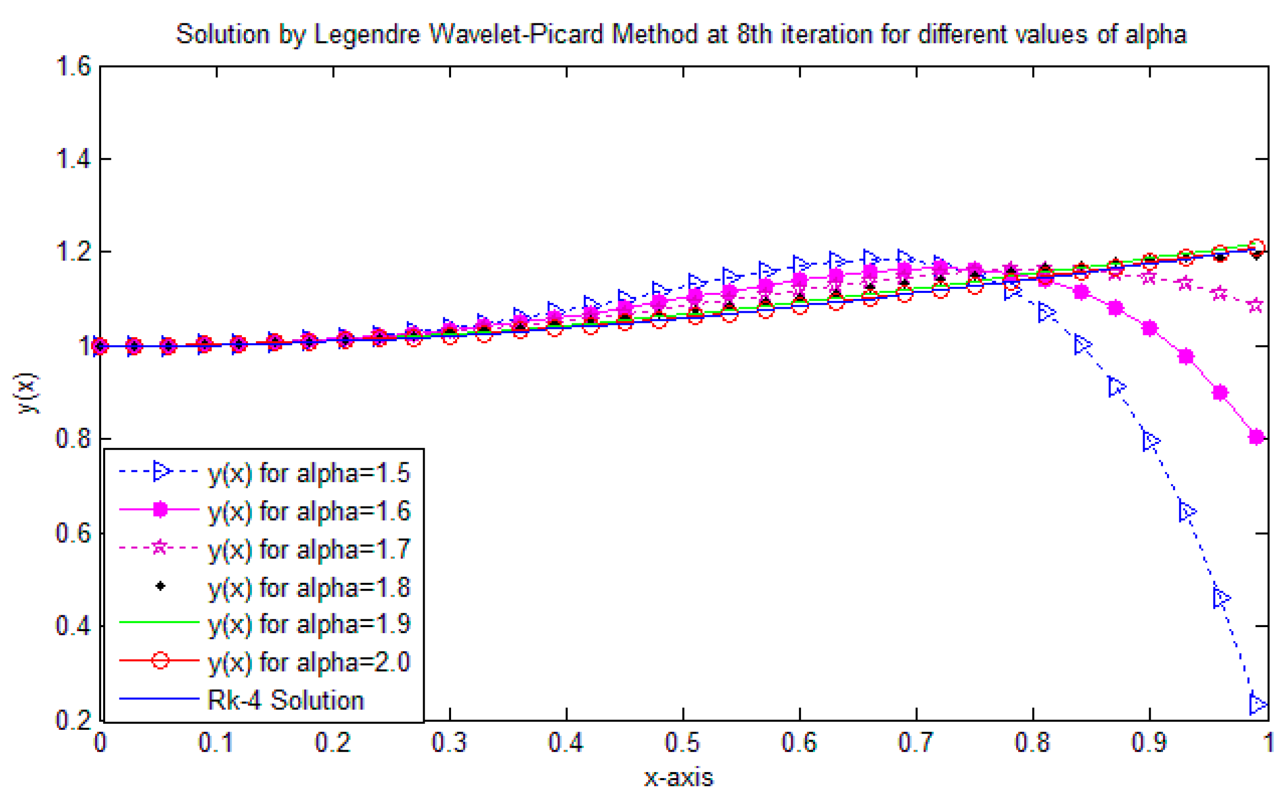
| VIM Solution | UWCM [24] Solution at M = 6 | LWPM Solution at M = 6 | RK-4 Solution | Error in UWCM [24] | Error in LWPM | |
|---|---|---|---|---|---|---|
| 0.0 | 1.00000000 | 1.00000000 | 1.00000000 | 1.00000000 | 1.0 × 10⁻¹⁰ | 1.2 × 10⁻¹³ |
| 0.1 | 1.00249660 | 1.00249669 | 1.00249669 | 1.00249670 | 1.1 × 10⁻⁸ | 1.0 × 10⁻⁸ |
| 0.2 | 1.00994530 | 1.00994541 | 1.00994542 | 1.00994545 | 4.0 × 10⁻⁸ | 3.1 × 10⁻⁸ |
| 0.3 | 1.02222113 | 1.02222170 | 1.02222174 | 1.02222179 | 9.0 × 10⁻⁸ | 5.9 × 10⁻⁸ |
| 0.4 | 1.03911114 | 1.03911438 | 1.03911446 | 1.03911459 | 2.1 × 10⁻⁷ | 1.3 × 10⁻⁷ |
| 0.5 | 1.06030866 | 1.06032195 | 1.06032214 | 1.06032231 | 3.6 × 10⁻⁷ | 1.7 × 10⁻⁷ |
| 0.6 | 1.08540584 | 1.08544861 | 1.08544887 | 1.08544906 | 4.5 × 10⁻⁷ | 1.9 × 10⁻⁷ |
| 0.7 | 1.11388470 | 1.11400052 | 1.11400072 | 1.11400108 | 5.6 × 10⁻⁷ | 3.6 × 10⁻⁷ |
| 0.8 | 1.14510669 | 1.14538393 | 1.14538393 | 1.14538468 | 7.5 × 10⁻⁷ | 7.5 × 10⁻⁷ |
| 0.9 | 1.17830101 | 1.17890549 | 1.17890570 | 1.17890664 | 1.1 × 10⁻⁶ | 9.4 × 10⁻⁷ |
| 1.0 | 1.21255189 | 1.21377602 | 1.21377710 | 1.21377819 | 2.1 × 10⁻⁶ | 1.1 × 10⁻⁶ |

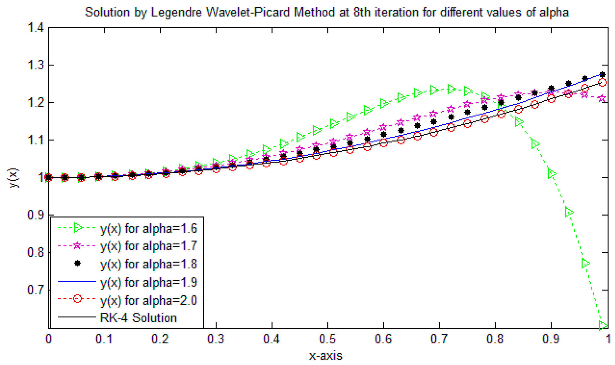
| VIM Solution | UWCM [24] Solution at M = 6 | LWPM Solution at M = 6 | RK-4 Solution | Error in UWCM [24] | Error in LWPM | |
|---|---|---|---|---|---|---|
| 0.0 | 1.00000000 | 1.00000000 | 1.00000000 | 1.00000000 | 1.0 × 10⁻⁹ | 1.0 × 10⁻¹¹ |
| 0.1 | 1.00250077 | 1.00250088 | 1.00250086 | 1.00250078 | 1.0 × 10⁻⁷ | 8.0 × 10⁻⁸ |
| 0.2 | 1.01001232 | 1.01001263 | 1.01001258 | 1.01001240 | 2.3 × 10⁻⁷ | 1.8 × 10⁻⁷ |
| 0.3 | 1.02256255 | 1.02256359 | 1.02256352 | 1.02256311 | 4.8 × 10⁻⁷ | 4.1 × 10⁻⁷ |
| 0.4 | 1.04019982 | 1.04020342 | 1.04020320 | 1.04020266 | 7.6 × 10⁻⁷ | 5.4 × 10⁻⁷ |
| 0.5 | 1.06299669 | 1.06300891 | 1.06300878 | 1.06300754 | 1.4 × 10⁻⁶ | 1.2 × 10⁻⁶ |
| 0.6 | 1.09105590 | 1.09109135 | 1.09109104 | 1.09108901 | 2.3 × 10⁻⁶ | 2.0 × 10⁻⁶ |
| 0.7 | 1.12451829 | 1.12460876 | 1.12460856 | 1.12460496 | 3.8 × 10⁻⁶ | 3.6 × 10⁻⁶ |
| 0.8 | 1.16357278 | 1.16377998 | 1.16377964 | 1.16377494 | 5.0 × 10⁻⁶ | 4.7 × 10⁻⁶ |
| 0.9 | 1.20846809 | 1.20890678 | 1.20890608 | 1.20890103 | 5.8 × 10⁻⁶ | 5.1 × 10⁻⁶ |
| 1.0 | 1.25952626 | 1.26040318 | 1.26040254 | 1.26039413 | 9.1 × 10⁻⁶ | 8.4 × 10⁻⁶ |

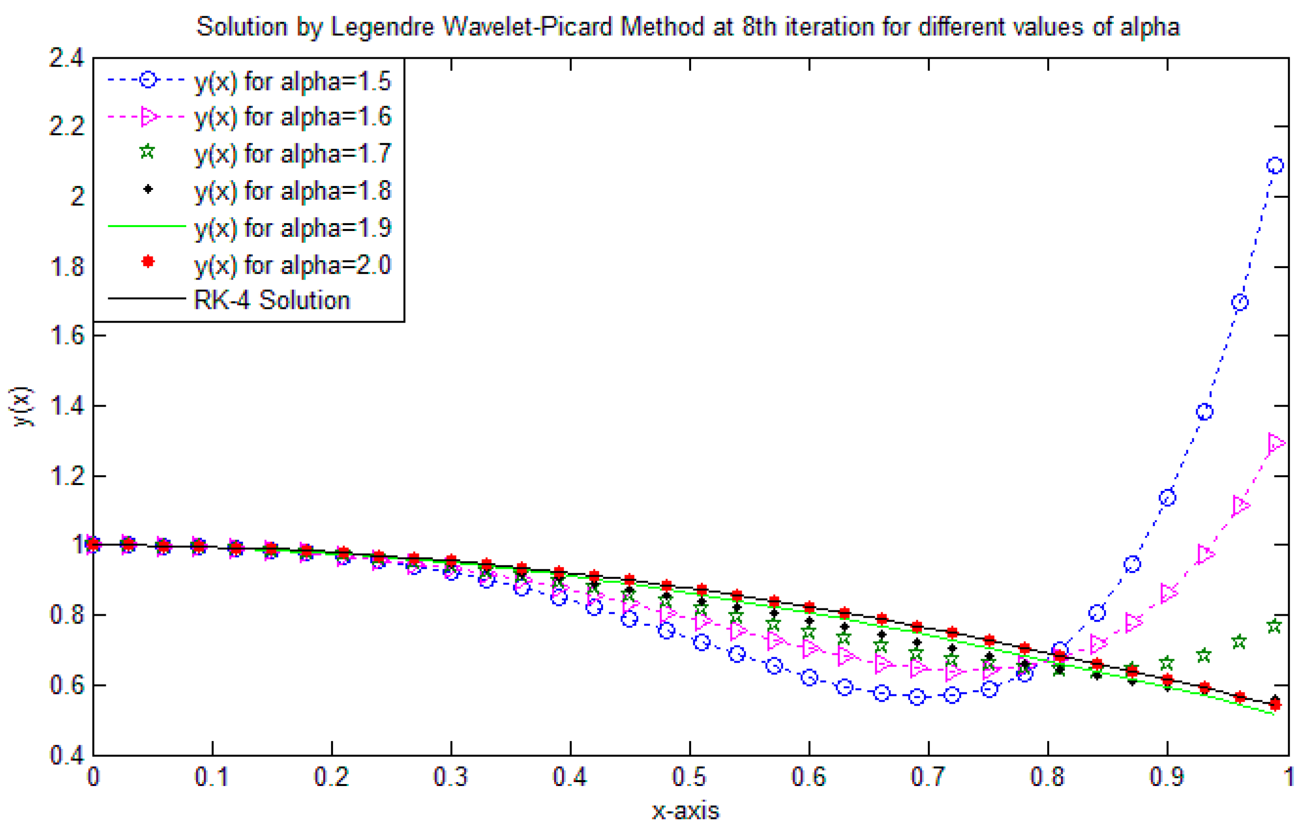
| VIM Solution | UWCM [24] Solution at M = 6 | LWPM Solution at M = 6 | RK-4 Solution | Error in UWCM [24] | Error in LWPM | |
|---|---|---|---|---|---|---|
| 0.0 | 1.00000000 | 1.00000000 | 1.00000000 | 1.00000000 | 1.0 × 10⁻⁹ | 1.2 × 10⁻⁹ |
| 0.1 | 0.99495428 | 0.99495428 | 0.99495427 | 0.99495427 | 1.0 × 10⁻⁸ | 7.0 × 10⁻⁹ |
| 0.2 | 0.97986771 | 0.97986769 | 0.97986765 | 0.97986761 | 8.0 × 10⁻⁸ | 4.1 × 10⁻⁸ |
| 0.3 | 0.95488865 | 0.95488784 | 0.95488778 | 0.95488770 | 1.4 × 10⁻⁷ | 8.3 × 10⁻⁸ |
| 0.4 | 0.92025739 | 0.92025265 | 0.92025256 | 0.92025243 | 2.2 × 10⁻⁷ | 1.3 × 10⁻⁷ |
| 0.5 | 0.87630062 | 0.87628321 | 0.87628308 | 0.87628280 | 4.1 × 10⁻⁷ | 2.8 × 10⁻⁷ |
| 0.6 | 0.82342666 | 0.82337721 | 0.82337705 | 0.82337636 | 8.5 × 10⁻⁷ | 6.9 × 10⁻⁷ |
| 0.7 | 0.76212192 | 0.76200270 | 0.76200234 | 0.76200157 | 1.1 × 10⁻⁶ | 7.7 × 10⁻⁷ |
| 0.8 | 0.69294873 | 0.69269483 | 0.69269436 | 0.69269338 | 1.5 × 10⁻⁶ | 9.8 × 10⁻⁷ |
| 0.9 | 0.61654510 | 0.61605312 | 0.61605226 | 0.61604996 | 3.1 × 10⁻⁶ | 2.3 × 10⁻⁶ |
| 1.0 | 0.53362658 | 0.53274003 | 0.53273896 | 0.53273066 | 9.3 × 10⁻⁶ | 8.3 × 10⁻⁶ |

| VIM Solution | UWCM [24] Solution at M = 6 | LWPM Solution at M = 6 | RK-4 Solution | Error in UWCM [24] | Error in LWPM | |
|---|---|---|---|---|---|---|
| 0.0 | 0.00000000 | 0.00000000 | 0.00000000 | 0.00000000 | 1.0 × 10⁻⁹ | 2.1 × 10⁻¹² |
| 0.1 | 0.19090972 | 0.19090974 | 0.19090975 | 0.19090978 | 4.0 × 10⁻⁸ | 3.0 × 10⁻⁸ |
| 0.2 | 0.38065613 | 0.38065651 | 0.38065653 | 0.38065658 | 7.0 × 10⁻⁸ | 5.0 × 10⁻⁸ |
| 0.3 | 0.56805809 | 0.56805941 | 0.56805942 | 0.56805959 | 1.8 × 10⁻⁷ | 1.7 × 10⁻⁷ |
| 0.4 | 0.75190092 | 0.75190395 | 0.75190402 | 0.75190437 | 4.2 × 10⁻⁷ | 3.5 × 10⁻⁷ |
| 0.5 | 0.93092454 | 0.93092998 | 0.93093003 | 0.93093096 | 9.8 × 10⁻⁷ | 9.3 × 10⁻⁷ |
| 0.6 | 1.10381762 | 1.10382601 | 1.10382611 | 1.10382756 | 1.6 × 10⁻⁶ | 1.4 × 10⁻⁶ |
| 0.7 | 1.26921875 | 1.26922885 | 1.26922919 | 1.26923100 | 2.1 × 10⁻⁶ | 1.9 × 10⁻⁶ |
| 0.8 | 1.42572628 | 1.42573213 | 1.42573263 | 1.42573479 | 2.7 × 10⁻⁶ | 2.1 × 10⁻⁶ |
| 0.9 | 1.57191725 | 1.57190182 | 1.57190210 | 1.57190495 | 3.1 × 10⁻⁶ | 2.8 × 10⁻⁶ |
| 1.0 | 1.70637581 | 1.70629821 | 1.70630014 | 1.70630325 | 5.0 × 10⁻⁶ | 3.1 × 10⁻⁶ |

4. Conclusions
Acknowledgments
Author Contributions
Conflicts of Interest
References
- Yang, X.J. Local Fractional Functional Analysis and Its Applications; Asian Academic Publisher Limited: Hong Kong, China, 2011. [Google Scholar]
- Yang, X.J. Local fractional integral transforms. Prog. Nonlinear Sci. 2011, 4, 1–225. [Google Scholar]
- Yang, X.J. Advanced Local Fractional Calculus and its Applications; World Science Publisher: New York, NY, USA, 2012. [Google Scholar]
- Malik, S.; Qureshi, I.M.; Zubair, M.; Haq, I. Solution to force-free and forced Duffing–van der Pol oscillator using memetic computing. J. Basic Appl. Sci. Res. 2012, 2, 1136–1148. [Google Scholar]
- Liu, G.R.; Wu, T.Y. Numerical solution for differential equations of duffing-type non-linearity using the generalized differential quadrature rule. J. Sound Vib. 2000, 237, 805–817. [Google Scholar] [CrossRef]
- Cordshooli, G.A.; Vahidi, A.R. Solutions of Duffing–van der Pol equation using decomposition method. Adv. Stud. Theor. Phys. 2011, 5, 121–129. [Google Scholar]
- El-Danaf, T.S.; Ramadan, M.A.; Alaal, A. The use of adomian decomposition method for solving the regularized long-wave equation. Chaos Soliton Fractals 2005, 26, 747–757. [Google Scholar] [CrossRef]
- Wazwaz, A.-M. Approximate solutions to boundary value problems of higher order by the modified decomposition method. Comp. Math. Appl. 2000, 40, 679–691. [Google Scholar] [CrossRef]
- Noor, M.A.; Mohyud-Din, S.T. Homotopy perturbation method for solving nonlinear higher-order boundary value problems. Int. J. Nonlinear Sci. Numer. Simul. 2008, 9, 395–408. [Google Scholar] [CrossRef]
- El-Wakil, S.A.; Madkour, M.A.; Abdou, M.A. Application of Exp-function method for nonlinear evolution equations with variable coefficient. Phys. Lett. A 2007, 369, 62–69. [Google Scholar] [CrossRef]
- Vázquez-Leal, H. Rational homotopy perturbation method. J. Appl. Math. 2012, 2012. [Google Scholar] [CrossRef]
- Noor, M.A.; Mohyud-Din, S.T. Variational iteration method for solving higher-order nonlinear boundary value problems using He’s polynomials. Int. J. Nonlinear Sci. Numer. Simul. 2008, 9, 141–156. [Google Scholar] [CrossRef]
- Saeed, U.; Rehman, M.U.; Iqbal, M.A. Haar Wavelet-Picard technique for fractional order nonlinear initial and boundary value problems. Sci. Res. Essays 2014, 9, 571–580. [Google Scholar]
- Cattani, C.; Kudreyko, A. Harmonic wavelet method towards solution of the Fredholm type integral equations of the second kind. Appl. Math. Comp. 2010, 215, 4164–4171. [Google Scholar] [CrossRef]
- Rawashdeh, E.A. Legendre wavelets method for fractional integro-differential equations. Appl. Math. Sci. 2011, 5, 2465–2474. [Google Scholar]
- Mohammadi, F.; Hosseini, M.M.; Mohyud-Din, S.T. Legendre wavelet Galerkin method for solving ordinary differential equations with non-analytic solution. Int. J. Syst. Sci. 2011, 42, 579–585. [Google Scholar] [CrossRef]
- Yousefi, S.; Banifatemi, A. Numerical solution of Fredholm integral equations by using CAS wavelets. Appl. Math. Comp. 2006, 183, 458–463. [Google Scholar] [CrossRef]
- Vasilyev, O.V.; Paolucci, S. A dynamically adaptative multilevel wavelet collocation method for solving partial differential equations in a finite domain. J. Comput. Phys. 1996, 125, 498–512. [Google Scholar] [CrossRef]
- Vasilyev, O.V.; Paolucci, S. A fast adaptive wavelet collocation algorithm for multidimensional PDEs. J. Comput. Phys. 1997, 138, 16–56. [Google Scholar] [CrossRef]
- Babolian, E.; Fattahzadeh, F. Numerical solution of differential equations by using Chebyshev wavelet operational matrix of integration. Appl. Math. Comput. 2007, 188, 417–426. [Google Scholar] [CrossRef]
- Venkatesh, S.G.; Ayyaswamy, S.K.; Balachandar, S.R. The Legendre wavelet method for solving initial value problems of Bratu-type. Comp. Math. Appl. 2012, 63, 1287–1295. [Google Scholar] [CrossRef]
- Abd-Elhameed, W.M.; Youssri, Y.H. New spectral solutions of multi-term fractional order initial value problems with error analysis. Comp. Model. Eng. Sci. 2015, 105, 375–398. [Google Scholar]
- Abd-Elhameed, W.M.; Doha, E.H.; Youssri, Y.H. New spectral second kind Chebyshev wavelets algorithm for solving linear and nonlinear second order differential equations involving singular and Bratu type equations. Abstr. Appl. Anal. 2013, 2013. [Google Scholar] [CrossRef]
- Youssri, Y.H.; Abd-Elhameed, W.M.; Doha, E.H. Ultraspherical wavelets method for solving Lane–Emden type equations. Romanian J. Phys. 2015, in press. [Google Scholar]
- Doha, E.H.; Abd-Elhameed, W.M.; Youssri, Y.H. New ultraspherical wavelets collocation method for solving 2nth-order initial and boundary value problems. J. Egypt. Math. Soc. 2015, in press. [Google Scholar] [CrossRef]
© 2015 by the authors; licensee MDPI, Basel, Switzerland. This article is an open access article distributed under the terms and conditions of the Creative Commons Attribution license (http://creativecommons.org/licenses/by/4.0/).
Share and Cite
Mohyud-Din, S.T.; Iqbal, M.A.; Hassan, S.M. Modified Legendre Wavelets Technique for Fractional Oscillation Equations. Entropy 2015, 17, 6925-6936. https://0-doi-org.brum.beds.ac.uk/10.3390/e17106925
Mohyud-Din ST, Iqbal MA, Hassan SM. Modified Legendre Wavelets Technique for Fractional Oscillation Equations. Entropy. 2015; 17(10):6925-6936. https://0-doi-org.brum.beds.ac.uk/10.3390/e17106925
Chicago/Turabian StyleMohyud-Din, Syed Tauseef, Muhammad Asad Iqbal, and Saleh M. Hassan. 2015. "Modified Legendre Wavelets Technique for Fractional Oscillation Equations" Entropy 17, no. 10: 6925-6936. https://0-doi-org.brum.beds.ac.uk/10.3390/e17106925