From Lattice Boltzmann Method to Lattice Boltzmann Flux Solver

Abstract

Based on the lattice Boltzmann method (LBM), the lattice Boltzmann flux solver (LBFS), which combines the advantages of conventional Navier–Stokes solvers and lattice Boltzmann solvers, was proposed recently. Specifically, LBFS applies the finite volume method to solve the macroscopic governing equations which provide solutions for macroscopic flow variables at cell centers. In the meantime, numerical fluxes at each cell interface are evaluated by local reconstruction of LBM solution. In other words, in LBFS, LBM is only locally applied at the cell interface for one streaming step. This is quite different from the conventional LBM, which is globally applied in the whole flow domain. This paper shows three different versions of LBFS respectively for isothermal, thermal and compressible flows and their relationships with the standard LBM. In particular, the performance of isothermal LBFS in terms of accuracy, efficiency and stability is investigated by comparing it with the standard LBM. The thermal LBFS is simplified by using the D2Q4 lattice velocity model and its performance is examined by its application to simulate natural convection with high Rayleigh numbers. It is demonstrated that the compressible LBFS can be effectively used to simulate both inviscid and viscous flows by incorporating non-equilibrium effects into the process for inviscid flux reconstruction. Several numerical examples, including lid-driven cavity flow, natural convection in a square cavity at Rayleigh numbers of 10⁷ and 10⁸ and transonic flow around a staggered-biplane configuration, are tested on structured or unstructured grids to examine the performance of three LBFS versions. Good agreements have been achieved with the published data, which validates the capability of LBFS in simulating a variety of flow problems.

1. Introduction

Since its earliest appearance in 1988 [1], the lattice Boltzmann equation (LBE)-based method [2,3,4,5,6,7,8,9,10,11] has been developed into an effective and efficient solver for simulating a variety of complex fluid flow problems, such as isothermal and thermal flows [9,10,12], multi-phase and multi-component flows [8,13,14,15], compressible flows [16,17,18] and micro non-equilibrium flows [19,20,21]. To effectively study these problems, a large number of LBE-based methods have been continuously proposed and refined [9,10,11,12,13,14,15,16,17,18,19,20,21,22,23].

Historically, the LBM was developed from the lattice gas cellular automata (LGCA) method, aiming to remove its statistical noise and limitation to use Boolean numbers. It was later proven that the solid foundation of LBM roots in gas kinetic theory and the Chapman–Enskog expansion analysis, through which both continuous and lattice Boltzmann equation can recover the Navier–Stokes equations. This confers the LBM with an appealing kinetic nature. Besides, LBM has very simple numerical algorithms with algebraic manipulations. In particular, two simple steps of streaming and collision are involved in its solution process. The streaming process is linear, which moves particles with different distribution functions to neighboring points, but effectively considers non-linear physics in fluid dynamics. The collision process takes place locally in either lattice velocity space or macroscopic moment space according to different collision models [2,4,22]. Both single relaxation time (SRT) model (lattice Bhatnagar–Gross–Krook (LBGK) model) [4] and multiple-relaxation-time (MRT) model [22] can be applied. It seems that the MRT model eliminates some defects of the LBGK model and enriches the connotation of LBM, although the computational effort is also increased. With these distinguishing features, the LBM has emerged as an alternative powerful tool in many complex fluid flow problems [13,20,23,24,25]. However, the LBM also suffers from some drawbacks. Due to lattice regularity, the standard LBM usually restricts its applications to uniform grids, which hinders its direct application in certain problems with curved boundaries. In addition, as compared with conventional Navier–Stokes solvers, LBM usually needs more virtual storage to store both the distribution functions and flow variables. Furthermore, the time step in LBM is coupled with mesh spacing, which presents a great challenge for applications on multi-block and adaptive grids. Moreover, LBM is mostly applied to simulate incompressible flows since the equilibrium distribution function is obtained from low Mach number approximation.

To remove the drawbacks of standard LBM, some efforts [5,6,7,21] have been made to directly solve the discrete velocity Boltzmann equation (DVBE) with well-established numerical approaches. This way eliminates the coupling issue between the mesh spacing and time step in standard LBM and can be effectively applied on non-uniform grids. However, it loses the primary advantages of LBM such as simple implementation and algebraic operation. It may also involve a large numerical dissipation and encounter numerical instability [26,27].

Recently, from Chapman–Enskog (C-E) analysis, several versions of lattice Boltzmann flux solver (LBFS) [8,9,10,11] have been developed based on the standard LBM for simulating isothermal, thermal, multiphase and compressible flows. LBFS is a finite volume solver for direct update of the macroscopic flow variables at cell centers. The key idea of the LBFS is to evaluate numerical fluxes at each cell interface by local application of LBM solution for one streaming step. In other words, in LBFS, LBM is applied locally and independently at each interface, and the streaming time step is nothing to do with the real time step. Instead, it is only applied to calculate the relaxation parameter used in the process of solution reconstruction by LBM. For a control cell with four cell interfaces of a two-dimensional case, the local LBM solution at different interface is reconstructed independently and the streaming time step could be different. This gives us a great flexibility for application of the solver to non-uniform meshes and complex geometry. This feature effectively removes the drawback of coupling issue between the mesh spacing and time step in the conventional LBM. In addition, the LBFS does not track the evolution of distribution function and the dependent variables are the macroscopic flow variable. As a consequence, the required virtual memory is reduced substantially, and the physical boundary conditions can be implemented directly without converting to those for distribution functions. Moreover, as compared with conventional incompressible Navier–Stokes solvers, such as the well-known semi-implicit method for pressure linked equations (SIMPLE) method and its variants [28], the LBFS overcomes their drawbacks of tedious discretization of the second order derivatives, the requirement of staggered grids for preventing pressure oscillations and slow convergence on fine grids [29]. Indeed, the LBFS combines the advantages of lattice Boltzmann solver (simplicity and kinetic nature) with those of Navier–Stokes solver by the finite volume method (FVM) (geometric flexibility and easy implementation of boundary conditions). It shows the progressive development from LBM to LBFS.

Since LBFS is a new solver, its performance has not been fully investigated and further improvements and simplifications for different flow problems may be required. Particularly, there is a lack of a systematic investigation on its accuracy, efficiency, stability and capability in simulating isothermal flows, thermal flows at high Reynolds/Rayleigh numbers, and compressible flows. Motived by this, the LBFS will be refined and examined comprehensively in this paper. Firstly, numerical simulations of two-dimensional lid-driven cavity flows [30,31,32,33,34] are considered. A detailed comparison of its performances with the standard LBM will be carried out. Secondly, the thermal LBFS will be simplified in this work by using the D2Q4 model and then applied to simulate natural convection at two high Rayleigh numbers of $Ra={10}^7{\text{ and 10}}^8$. The obtained results on different grids will be compared with those by MRT-based LBM [35]. Thirdly, the compressible LBFS will be improved by incorporating non-equilibrium effects into the process for inviscid flux reconstruction and introducing a switch function to control numerical diffusion. Its performance will be examined by simulating transonic inviscid and viscous flows around a staggered-biplane configuration on unstructured grids. The obtained results will be compared with the published data.

2. Lattice Boltzmann Method

For a general case, we consider incompressible thermal fluid flows and the LBE with BGK approximation can be written as [34,36]:

$$f_{\alpha }(\mathit{r}+{\mathit{e}}_{\alpha }{\delta }_t,t+{\delta }_t)=f_{\alpha }(\mathit{r},t)+\frac{f_{\alpha }^{eq}(\mathit{r},t)-f_{\alpha }(\mathit{r},t)}{{\tau }_v},\alpha =0,1,\mathrm{...},N,$$

(1)

$$g_{\alpha }(\mathit{r}+{\mathit{e}}_{\alpha }{\delta }_t,t+{\delta }_t)=g_{\alpha }(\mathit{r},t)+\frac{g_{\alpha }^{eq}(\mathit{r},t)-g_{\alpha }(\mathit{r},t)}{{\tau }_c},\alpha =0,1,\mathrm{...},M,$$

(2)

where $f_{\alpha }$ and $g_{\alpha }$ are density distribution functions (DDF) and temperature distribution functions (TDF) respectively; $f_{\alpha }^{eq}$ and $g_{\alpha }^{eq}$ are equilibrium states of $f_{\alpha }$ and $g_{\alpha }$; ${\tau }_v$ and ${\tau }_c$ are relaxation parameters; ${\delta }_t$ is the streaming time; $M$ and $N$ are the total number of discrete particles for $f_{\alpha }$ and $g_{\alpha }$. The macroscopic fluid properties of density $\rho$, velocity $\mathit{u}$ and temperature $T$ are evaluated from lattice moments of $f_{\alpha }$ and $g_{\alpha }$:

$$\rho ={\displaystyle \sum _{\alpha =0}^N{f}_{\alpha }}, \rho \mathit{u}={\displaystyle \sum _{\alpha =0}^N{f}_{\alpha }}{\mathit{e}}_{\alpha }, T={\displaystyle \sum _{\alpha =0}^M{g}_{\alpha }}$$

(3)

The equilibrium DDF $f_{\alpha }^{eq}$ is given by [4]:

$$f_{\alpha }^{eq}\left(\mathit{r},t\right)=\rho w_{\alpha }\left[1+\frac{{\mathit{e}}_{\alpha }\cdot \mathit{u}}{c_s^2}+\frac{{\left({\mathit{e}}_{\alpha }\cdot \mathit{u}\right)}^2-{\left(c_s\left|\mathit{u}\right|\right)}^2}{2c_s^4}\right]$$

(4)

The D2Q9 model, whose lattice components are written as ${\mathit{e}}_{\alpha }=\left(0,0\right),$ $\left(\pm 1,0\right)$, $\left(0,\pm 1\right)$ and $\left(\pm 1,\pm 1\right)$, is commonly applied for $f_{\alpha }^{eq}$. The weights $w_{\alpha }$ and the sound speed $c_s$ in Equation (4) are $w_0=4/9$, $w_{1~4}=1/9$, $w_{5~8}=1/36$ and $c_s=1/\sqrt{3}$. The equilibrium TDF $g_{\alpha }^{eq}$ is given by [37]:

$$g_{\alpha }^{eq}\left(\mathit{r},t\right)=\frac{T}{4}\left[1+2{\mathit{e}}_{\alpha }\cdot \mathit{u}\right]$$

(5)

The D2Q4 lattice velocity model, whose lattice components are written as ${\mathit{e}}_{\alpha }=\left(\pm 1,\pm 1\right)$, is usually used for $g_{\alpha }^{eq}$. ${\tau }_{\nu }$ and ${\tau }_c$ are respectively calculated by the dynamic viscosity $\mu$ and thermal diffusivity $\kappa$:

$$\mu =\left({\tau }_{\nu }-\frac{1}{2}\right)\rho c_s^2{\delta }_t$$

(6a)

$$\kappa =\frac{1}{2}\left({\tau }_c-\frac{1}{2}\right){\delta }_t$$

(6b)

Note that Equations (1) and (2) are applied to simulate thermal flows. If isothermal flows are considered, we can just apply Equation (1). For the application of LBM, we have to apply Equations (1) and (2) in the whole computational domain and track the evolution of distribution functions $f_{\alpha }$ and $g_{\alpha }$. In addition, physical boundary conditions for macroscopic variables are converted to those for $f_{\alpha }$ and $g_{\alpha }$. For no-slip condition, bounce-back scheme can be easily applied. In some cases, accurate implementation of other boundary conditions in the LBM may not be as straightforward as in Navier–Stokes solvers.

3. Chapman–Enskog Analysis

As a mesoscopic method with microscopic particle distribution functions, the LBM described in Section 2 has been well applied to study weakly compressible fluid flows in incompressible limit. Conventionally, such flows are governed and solved by the macroscopic conservation laws of mass, momentum and energy. This indicates that the solution of a physical flow problem can be either obtained by applying the mesoscopic LBM or the macroscopic Navier–Stokes solver. It is interesting to note that these two intrinsically different numerical methods, one from microscopic statistical physics and the other from macroscopic conservation laws, are both able to study the same fluid flow problem. From this point of view, it can be inferred that these two methods should have some connections. Indeed, it has been proven that the lattice Boltzmann equation is able to recover the Navier–Stokes equation through the multi-scale Chapman–Enskog expansion analysis, which is briefly introduced below.

A multi-scale expansion of the DDF, TDF, the temporal derivative and the spatial derivative can be respectively given by:

$$f_{\alpha }=f_{\alpha }^{(0)}+\epsilon f_{\alpha }^{(1)}+{\epsilon }^2{f}_{\alpha }^{(2)}$$

(7a)

$$g_{\alpha }=g_{\alpha }^{(0)}+\epsilon g_{\alpha }^{(1)}+{\epsilon }^2{g}_{\alpha }^{(2)}$$

(7b)

$$\frac{\partial }{\partial t}=\epsilon \frac{\partial }{\partial t_0}+{\epsilon }^2\frac{\partial }{\partial t_1}$$

(7c)

$${\nabla }_r=\epsilon {\nabla }_{r1}$$

(7d)

where ε is a small parameter proportional to the Knudsen number. Applying the second order Taylor-series expansion to Equations (1) and (2) gives:

$$(\frac{\partial }{\partial t}+{\mathit{e}}_{\alpha }\cdot \nabla )f_{\alpha }+\frac{{\delta }_t}{2}{(\frac{\partial }{\partial t}+{\mathit{e}}_{\alpha }\cdot \nabla )}^2{f}_{\alpha }+\frac{1}{\tau {\delta }_t}(f_{\alpha }-f_{\alpha }^{eq})+O({\delta }_t^2)=0,$$

(8)

$$(\frac{\partial }{\partial t}+{\mathit{e}}_{\alpha }\cdot \nabla )g_{\alpha }+\frac{{\delta }_t}{2}{(\frac{\partial }{\partial t}+{\mathit{e}}_{\alpha }\cdot \nabla )}^2{g}_{\alpha }+\frac{1}{\tau {\delta }_t}(g_{\alpha }-g_{\alpha }^{eq})+O({\delta }_t^2)=0.$$

(9)

The macroscopic Navier–Stokes equations for conservation laws can be recovered by substituting Equation (7) into Equations (8) and (9) [9,10]:

$$\frac{\partial W}{\partial t}+\mathbf{\nabla }\cdot F=0$$

(10)

where:

$$W=\left\{\begin{array}{c}\rho \\ \rho \mathit{u}\\ T\end{array}\right\} \mathrm{and} F=\left\{\begin{array}{c}\mathit{P}\\ \mathbf{\Pi }\\ \mathit{Q}\end{array}\right\}$$

(11)

In Equation (11), $\mathit{P},\mathbf{\Pi }$ and $\mathit{Q}$ are respectively mass, momentum and energy fluxes and can be given by lattice summations of DDFs and TDFs [9,10]:

$$\mathit{P}=\rho \mathit{u}={\displaystyle \sum _{\alpha =0}^N{f}_{\alpha }^{eq}{\mathit{e}}_{\alpha }}$$

(12a)

$$\mathbf{\Pi }=\rho u\otimes u+pI-\mu \left(\nabla u+{\left(\nabla u\right)}^T\right)={\displaystyle \sum _{\alpha =0}^N{\mathit{e}}_{\alpha }{\mathit{e}}_{\alpha }{f}_{\alpha }^{^}}$$

(12b)

$$\mathit{Q}=\mathit{u}T-\kappa \nabla T={\displaystyle \sum _{\alpha =0}^N{\mathit{e}}_{\alpha }{g}_{\alpha }^{^}}$$

(12c)

where:

$$f_{\alpha }^{^}=f_{\alpha }^{eq}+\left(1-\frac{1}{2{\tau }_{\nu }}\right)f_{\alpha }^{neq} \mathrm{and} g_{\alpha }^{^}=g_{\alpha }^{eq}+\left(1-\frac{1}{2{\tau }_c}\right)g_{\alpha }^{neq}$$

(13)

$$f_{\alpha }^{neq}\text{= }-{\tau }_{\nu }{\delta }_t\left(\frac{\partial }{\partial t}+{\mathit{e}}_{\alpha }\cdot \nabla \right)f_{\alpha }^{eq}$$

(14a)

$$g_{\alpha }^{neq}\text{= }-{\tau }_c{\delta }_t\left(\frac{\partial }{\partial t}+{\mathit{e}}_{\alpha }\cdot \nabla \right)g_{\alpha }^{eq}$$

(14b)

In the conventional LBM, the Chapman–Enskog (C-E) analysis is usually used to verify that the flow variables obtained by LBM can satisfy the macroscopic Navier–Stokes equations. In some interesting works, this C-E analysis is also applied to build a hybrid solver by combing the LBM with the FVM scheme for Navier–Stokes equations [37,38,39]. In our recent work [9,10], it was found that the relationship between flow variables/fluxes and particle distribution functions given in Equation (12) can be applied to build a new solver named LBFS with a better performance, which effectively combines the advantages of Navier–Stokes solver and lattice Boltzmann solver and at the same time removes some of their drawbacks. The reliability and flexibility of the LBFS have been demonstrated in [8,9,10].

4. LBFS for Isothermal and Thermal Incompressible Flows

Based on the LBM given by Equations (1) and (2), the LBFS [9] has been proposed by solving Equation (10) directly. Unlike conventional Navier–Stokes solver, which applies well-established schemes to discretize Equation (10), the LBFS is a finite volume solver and reconstructs its fluxes locally with Equation (12) derived from Chapman–Enskog analysis. It may be pointed out that Equation (12) for flux reconstruction can be applied with different lattice velocity models. In our previous work [9], the D2Q9 thermal model for temperature field is applied, which is obviously complex and inefficient as compared with the D2Q4 model [34]. In this work, this drawback will be removed by applying the D2Q4 model. The details are given below.

4.1. Finite Volume Discretization

A finite volume discretization of Equation (10) over a control volume ${\text{Ω}}_i$ gives the following formulation:

$$\frac{d{W}_i}{dt}=-\frac{1}{d{V}_i}{\displaystyle \sum _k{R}_{k}d{l}_k}, R_k={\left(\mathit{n}\cdot F\right)}_k$$

(15)

where $d{V}_i$ is the area of the control cell ${\text{Ω}}_i$, $d{l}_k$ is the length of the k-th control surface enclosed ${\text{Ω}}_i$ and $\mathit{n}=\left(n_x,n_y\right)$ is the unit normal vector on the k-th control surface. With the D2Q9 and D2Q4 models, the flux $R_k$ at each cell interface can be written as follows:

$$R_k={\left(\begin{array}{c}{n}_x\left(f_1^{eq}-f_3^{eq}+f_5^{eq}-f_6^{eq}-f_7^{eq}+f_8^{eq}\right)+n_y\left(f_2^{eq}-f_4^{eq}+f_5^{eq}+f_6^{eq}-f_7^{eq}-f_8^{eq}\right)\\ n_x\left(f_1^{^}\text{+}{f}_3^{^}\text{+}{f}_5^{^}\text{+}{f}_6^{^}\text{+}{f}_7^{^}\text{+}{f}_8^{^}\right)\text{+}{n}_y\left(f_5^{^}-f_6^{^}\text{+}{f}_7^{^}-f_8^{^}\right)\\ n_x\left(f_5^{^}-f_6^{^}\text{+}{f}_7^{^}-f_8^{^}\right)\text{+}{n}_y\left(f_2^{^}\text{+}{f}_4^{^}\text{+}{f}_5^{^}\text{+}{f}_6^{^}\text{+}{f}_7^{^}\text{+}{f}_8^{^}\right)\\ n_x\left(g_1^{^}-g_3^{^}\right)+n_y\left(g_2^{^}-g_4^{^}\right)\end{array}\right)}_k$$

(16)

As can be seen, the formulation of the energy flux reconstructed by the simplified D2Q4 lattice velocity model is much simpler than that given by the original D2Q9 model [9]. In Equation (16), the unknowns are $f_{\alpha }^{^}$ and $g_{\alpha }^{^}$ defined in Equation (13), which include both equilibrium and non-equilibrium density and temperature distribution functions $f_{\alpha }^{eq}$, $f_{\alpha }^{neq}$, $g_{\alpha }^{eq}$ and $g_{\alpha }^{neq}$. All these unknowns can be obtained through local reconstruction of the LBE solution without tracking the evolution of the DDF and TDF.

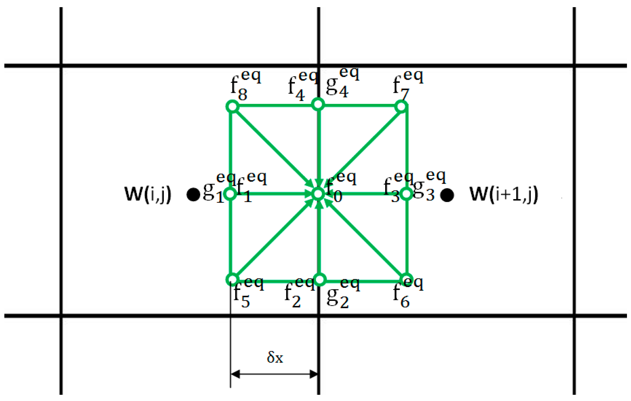
4.2. Local Reconstruction of Fluxes at Each Interface

Figure 1 shows an interface between two adjacent control cells for local reconstruction of fluxes [10], in which the D2Q9 and D2Q4 lattice velocity models respectively for DDF and TDF are embedded. The non-equilibrium parts for DDF and TDF are given by Equation (14). At each cell interface, discretization of Equation (14) with the second-order Taylor-series expansion gives the following equations [9]:

$$f_{\alpha }^{neq}(\mathit{r},t)=-{\tau }_{\nu }\left[f_{\alpha }^{eq}(\mathit{r},t)-f_{\alpha }^{eq}(\mathit{r}-{\mathit{e}}_{\alpha }{\delta }_t,t-{\delta }_t)\right]$$

(17a)

$$g_{\alpha }^{neq}(\mathit{r},t)=-{\tau }_c\left[g_{\alpha }^{eq}(\mathit{r},t)-g_{\alpha }^{eq}(\mathit{r}-{\mathit{e}}_{\alpha }{\delta }_t,t-{\delta }_t)\right]$$

(17b)

where $\mathit{r}$ represents the location of the cell interface. Equation (17) shows that both $f_{\alpha }^{neq}$ and $g_{\alpha }^{neq}$ can be approximated from $f_{\alpha }^{eq}$ and $g_{\alpha }^{eq}$ at the interface and its surrounding points $\mathit{r}-{\mathit{e}}_{\alpha }{\delta }_t$. Following the convention in LBM, $f_{\alpha }^{eq}$ and $g_{\alpha }^{eq}$ at the position and time $(\mathit{r}-{\mathit{e}}_{\alpha }{\delta }_t,t-{\delta }_t)$ are computed by using Equations (4) and (5). The involved flow quantities of density $\rho$, velocity $\mathit{u}$ and temperature $T$ at $\left(\mathit{r}-{\mathit{e}}_{\alpha }{\delta }_t,t-{\delta }_t\right)$ can be obtained through interpolations:

$$\psi (\mathit{r}-{\mathit{e}}_{\alpha }{\delta }_t,t-{\delta }_t)=\{\begin{array}{l}\psi ({\mathit{r}}_i)+(\mathit{r}-{\mathit{e}}_{\alpha }{\delta }_t-{\mathit{r}}_i)\mathbf{·}\nabla \psi ({\mathit{r}}_i),\text{ when }\mathit{r}-{\mathit{e}}_{\alpha }{\delta }_t\text{ is in }{\mathrm{\Omega }}_i\hfill \\ \psi ({\mathit{r}}_{i+1})+(\mathit{r}-{\mathit{e}}_{\alpha }{\delta }_t-{\mathit{r}}_{i+1})\mathbf{·}\nabla \psi ({\mathit{r}}_{i+1}),\text{ when }\mathit{r}-{\mathit{e}}_{\alpha }{\delta }_t\text{ is in }{\mathrm{\Omega }}_{i+1}\hfill \end{array}$$

(18)

where ${\mathit{r}}_i$ and ${\mathit{r}}_{i+1}$ are the locations of the two cell centers and $\psi$ represents any of the flow variables. After interpolation, $f_{\alpha }^{eq}(\mathit{r}-{\mathit{e}}_{\alpha }{\delta }_t,t-{\delta }_t)$ and $g_{\alpha }^{eq}(\mathit{r}-{\mathit{e}}_{\alpha }{\delta }_t,t-{\delta }_t)$ can be obtained.

Figure 1. Evaluation of flux at an interface between two control cells.

Figure 1. Evaluation of flux at an interface between two control cells.

Similarly, $f_{\alpha }^{eq}\left(\mathit{r},t\right)$ and $g_{\alpha }^{eq}\left(\mathit{r},t\right)$ can be calculated by Equations (4) and (5) if macroscopic flow variables are known. So, the challenging issue is to evaluate $\rho$, $\mathit{u}$ and $T$ at the cell interface $\left(\mathit{r},t\right)$. Previous studies [9,10] have shown that they can be reconstructed locally by streaming the particle from the neighboring point $(\mathit{r}-{\mathit{e}}_{\alpha }{\delta }_t,t-{\delta }_t)$ to the cell interface. As a result, we have:

$$\rho (\mathit{r},t)={\displaystyle \sum _{\alpha =0}^N{f}_{\alpha }^{eq}(\mathit{r}-{\mathit{e}}_{\alpha }{\delta }_t,t-{\delta }_t)},$$

(19a)

$$\rho (\mathit{r},t)\mathit{u}(\mathit{r},t)={\displaystyle \sum _{\alpha =0}^N{f}_{\alpha }^{eq}(\mathit{r}-{\mathit{e}}_{\alpha }{\delta }_t,t-{\delta }_t){\mathit{e}}_{\alpha }}$$

(19b)

$$T(\mathit{r},t)={\displaystyle \sum _{\alpha =0}^N{g}_{\alpha }^{eq}(\mathit{r}-{\mathit{e}}_{\alpha }{\delta }_t,t-{\delta }_t)}$$

(19c)

With the flow quantities obtained from Equation (19), $f_{\alpha }^{eq}\left(\mathit{r},t\right)$ and $g_{\alpha }^{eq}\left(\mathit{r},t\right)$ can be computed by using Equations (4) and (5). Once $f_{\alpha }^{eq}$, $f_{\alpha }^{neq}$, $g_{\alpha }^{eq}$ and $g_{\alpha }^{neq}$ are obtained, the fluxes at each cell interface can be evaluated numerically. Then Equation (15) can be solved by conventional Runge–Kutta scheme.

5. LBFS for Compressible Flows

5.1. Navier–Stokes Equations Discretized by FVM and Compressible Lattice Boltzmann Model

In Section 4, the local LBM solution is reconstructed by using the conventional lattice Boltzmann model, which is limited to incompressible flows. Thus, LBFS in Section 4 can only be applied to simulate incompressible flows. To simulate compressible flows by LBFS, we need to use the compressible lattice Boltzmann model to reconstruct the solution at the cell interface. However, the existing compressible lattice Boltzmann models are very complicated and inefficient for 2D and 3D cases. To simplify the solution process and make LBFS be applicable for simulation of compressible flows, we apply the 1D compressible lattice Boltzmann model along the normal direction of cell interface to evaluate the inviscid flux, and the viscous flux is still approximated by conventional finite difference schemes. This process is equivalent to developing a Riemann solver by 1D compressible lattice Boltzmann model.

In LBFS, the Navier–Stokes equations are discretized by FVM and the fluxes at the cell interface are evaluated by local reconstruction of LBM solutions [11]. Thanks to the application of FVM, it is convenient for LBFS to apply on arbitrary meshes. The compressible Navier–Stokes equations discretized by FVM can be written as:

$$\frac{d{W}_i}{dt}=-\frac{1}{d{V}_i}{\displaystyle \sum _{k=1}^{N_f}\left(F_{ck}-F_{vk}\right)d{l}_k}$$

(20)

where i is the index of a control volume, $d{V}_i$ and $N_f$ represent the volume and the number of interfaces of the control volume i, respectively. $W$, $F_c$ and $F_v$ are the conservative variables at the cell center and the inviscid and viscous fluxes at the cell interface given by:

$$W=\left[\begin{array}{c}\rho \\ \rho u\\ \rho v\\ \rho E\end{array}\right], F_c=\left[\begin{array}{c}\rho U_n\\ \rho u{U}_n+n_{x}p\\ \rho v{U}_n+n_{y}p\\ \left(\rho E+p\right)U_n\end{array}\right], F_v=\left[\begin{array}{c}0\\ n_x{\tau }_{xx}+n_y{\tau }_{xy}\\ n_x{\tau }_{yx}+n_y{\tau }_{yy}\\ n_x{\mathrm{\Theta }}_x+n_y{\mathrm{\Theta }}_y\end{array}\right]$$

(21)

Here, $\rho$ and $p$ are the density and pressure of mean flow, respectively. $(u,v)$ and $(n_x,n_y)$ denote the velocity vector and unit normal vector on the control surface in the Cartesian coordinate system, respectively. $E$ is the total energy of mean flow. $U_n$ represents the normal velocity. Furthermore, ${\tau }_{ij}$ denotes the components of viscous stress tensor and ${\mathrm{\Theta }}_i$ represents the term describing the work of viscous stress and the heat conduction in the fluid.

To compute $F_c$ by LBFS, the compressible lattice Boltzmann model is required. In this work, the non-free parameter D1Q4 model [11] is utilized. The configuration of this model is shown in Figure 2, and it is given by:

$$\begin{array}{l}{g}_1=\frac{\rho \left(-d_1{d}_2^2-d_2^{2}u+d_1{u}^2+d_1{c}^2+u^3+3u{c}^2\right)}{2d_1\left(d_1^2-d_2^2\right)}\\ g_2=\frac{\rho \left(-d_1{d}_2^2+d_2^{2}u+d_1{u}^2+d_1{c}^2-u^3-3u{c}^2\right)}{2d_1\left(d_1^2-d_2^2\right)}\\ g_3=\frac{\rho \left(d_1^2{d}_2+d_1^{2}u-d_2{u}^2-d_2{c}^2-u^3-3u{c}^2\right)}{2d_2\left(d_1^2-d_2^2\right)}\\ g_4=\frac{\rho \left(d_1^2{d}_2-d_1^{2}u-d_2{u}^2-d_2{c}^2+u^3+3u{c}^2\right)}{2d_2\left(d_1^2-d_2^2\right)}\end{array}$$

(22)

$$\begin{array}{l}{d}_1=\sqrt{u^2+3c^2-\sqrt{4u^2{c}^2+6c^4}}\\ d_2=\sqrt{u^2+3c^2+\sqrt{4u^2{c}^2+6c^4}}\end{array}$$

(23)

where $c$ represents the peculiar velocity of particles defined as $c=\sqrt{p/\rho }$. Note that in Equation (22), g is the equilibrium distribution function $f^{eq}$. As D1Q4 model is a one-dimensional model, it needs to be applied along the normal direction of cell interface for multi-dimensional problems [11]. That is, the velocity u in Equations (22) and (23) should be replaced by normal velocity $U_n$ when multi-dimensional problems are considered.

Figure 2. Configuration of non-free parameter D1Q4 model.

Figure 2. Configuration of non-free parameter D1Q4 model.

Suppose that the cell interface is located at $r=0$. For simplicity, a local-coordinate system with x-axis pointing to the normal direction and y-axis pointing to the tangential direction of the cell interface is used. As a result, the inviscid flux at the cell interface in the local-coordinate system can be written as:

$$F_c^{*}={\left[\begin{array}{cccc}\rho U_n& \rho U_n{U}_n+p& \rho U_n{U}_{\tau }& \left(\rho E+p\right)U_n\end{array}\right]}^T=F_c^n+F_c^t$$

(24a)

$$F_c^n={\left[\begin{array}{cccc}\rho U_n& \rho U_n{U}_n+p& 0& \left(\rho \left(\frac{1}{2}{U}_n^2+e\right)+p\right)U_n\end{array}\right]}^T$$

(24b)

$$F_c^t={\left[\begin{array}{cccc}0& 0& \rho U_n{U}_{\tau }& \frac{1}{2}\rho U_{\tau }^2{U}_n\end{array}\right]}^T$$

(24c)

Here, $F_c^n$ and $F_c^t$ are respectively the flux attributed to the normal velocity and tangential velocity, $e$ is the potential energy of mean flow. From Chapman–Enskog analysis, and with the use of non-free parameter D1Q4 model, $F_c^n$ can be computed by:

$$F_c^n={\displaystyle \sum _{i=1}^4{\xi }_i{\mathbf{\phi }}_i{f}_i\left(0,t\right)}$$

(25)

where:

$$f_i\left(0,t\right)=f^{eq}\left(0,t\right)+f^{neq}\left(0,t\right)=g_i\left(0,t\right)-{\tau }_0\left[g_i\left(0,t\right)-g_i\left(-{\xi }_i\delta t,t-\delta t\right)\right],$$

(26)

${\xi }_i$ is the particle velocity in the $i$-direction, i.e., ${\xi }_1=d_1$, ${\xi }_2=-d_1$, ${\xi }_3=d_2$ and ${\xi }_4=-d_2$. ${\mathbf{\phi }}_i$ stands for the moments:

$${\mathbf{\phi }}_i={\left(1,{\xi }_i,0,\frac{1}{2}{\xi }_i^2+e_p\right)}^T$$

(27)

Here, $e_p$ is the potential energy of particles; $f_i(0,t)$ is the distribution function at the cell interface. $g_i(0,t)$ and $g_i(-{\xi }_i\delta t,t-\delta t)$ are respectively the equilibrium distribution function at the cell interface and the surrounding point of the cell interface. The non-equilibrium part in Equation (26) is viewed as the numerical dissipation since only the inviscid flux is computed by LBFS. ${\tau }_0$ is the dimensionless collision time, which can be regarded as the weight of the numerical dissipation [40,41]. Substituting Equation (26) into Equation (25), we have the final expression of $F_c^n$ as follows:

$$F_c^n=\left(1-{\tau }_0\right)F_c^{n,I}+{\tau }_0{F}_c^{n,II}$$

(28)

where:

$$F_c^{n,I}={\displaystyle \sum _{i=1}^4{\xi }_i{\mathbf{\phi }}_a{g}_i\left(0,t\right)} \mathrm{and} F_c^{n,II}={\displaystyle \sum _{i=1}^4{\xi }_i{\mathbf{\phi }}_a{g}_i\left(-{\xi }_i\delta t,t-\delta t\right)}$$

(29)

To evaluate the flux attributed to the tangential velocity, one of the feasible ways can be expressed as:

$$F_c^t(3)={\displaystyle \sum _{i=1,3}{\xi }_i{f}_i\left(0,t\right)U_{\tau }^L}+{\displaystyle \sum _{i=2,4}{\xi }_i{f}_i\left(0,t\right)U_{\tau }^R}$$

(30a)

$$F_c^t(4)=\frac{1}{2}\left[{\displaystyle \sum _{i=1,3}{\xi }_i{f}_i\left(0,t\right){\left(U_{\tau }^L\right)}^2}+{\displaystyle \sum _{i=2,4}{\xi }_i{f}_i\left(0,t\right){\left(U_{\tau }^R\right)}^2}\right]$$

(30b)

where, $U_{\tau }^L$ and $U_{\tau }^R$ are the tangential velocity at the left and right side of cell interface, respectively. From $F_c^{*}$, the actual inviscid flux $F_c$ in Equation (20) in the Cartesian coordinate system can be obtained by a transformation [41]:

$$F_c=[\begin{array}{cccc}{F}_c^{*}(1)& F_c^{*}(2)n_x-F_c^{*}(3)n_y& F_c^{*}(2)n_y+F_c^{*}(3)n_x& F_c^{*}(4)\end{array}]$$

(31)

Equation (31) forms the LBFS for inviscid compressible flows. It can be treated as a Riemann solver developed by 1D compressible lattice Boltzmann model. As for the viscous flux $F_v$, it is still approximated by conventional finite difference schemes in this work.

5.2. Evaluation of Inviscid Flux by LBFS

To compute $F_c^{n,I}$, the equilibrium distribution function at the cell interface should be computed in advance. As the equilibrium distribution function is the function of conservative variables, we just need to calculate the conservative variables at the cell interface first. The conservative variables at the cell interface in the local-coordinate system can be expressed as:

$$W^{*}={\left[\begin{array}{cccc}\rho & \rho U_n& \rho U_{\tau }& \rho E\end{array}\right]}^T=W^n+W^t$$

(32a)

$$W^n={\left[\begin{array}{cccc}\rho & \rho U_n& 0& \rho \left(\frac{1}{2}{U}_n^2+e\right)\end{array}\right]}^T$$

(32b)

$$W^t={\left[\begin{array}{cccc}0& 0& \rho U_{\tau }& \frac{1}{2}\rho U_{\tau }^2\end{array}\right]}^T$$

(32c)

Like Equation (19), the conservative variables at the cell interface attributed to the normal velocity can be evaluated by:

$$W^n={\displaystyle \sum _{i=1}^4{\mathbf{\phi }}_i{g}_i\left(-{\xi }_i\delta t,t-\delta t\right)}$$

(33)

It is assumed that a local Riemann problem is formed at the cell interface. Then, the equilibrium distribution function $g_i\left(-{\xi }_i\delta t,t-\delta t\right)$ can be given by:

$$g_i\left(-{\xi }_i\delta t,t-\delta t\right)=\{\begin{array}{c}{g}_i^L\text{ if }i=1,3\\ g_i^R\text{ if }i=2,4\end{array}$$

(34)

where $g_i^L$ and $g_i^R$ are the equilibrium distribution functions at the left and right sides of cell interface as shown in Figure 3. In addition, the conservative variables attributed to the tangential velocity can be approximated by:

$$W^t(3)={\displaystyle \sum _{i=1,3}{g}_i\left(-{\xi }_i\delta t,t-\delta t\right)U_{\tau }^L}+{\displaystyle \sum _{i=2,4}{g}_i\left(-{\xi }_i\delta t,t-\delta t\right)U_{\tau }^R}$$

(35a)

$$W^t(4)=\frac{1}{2}\left[{\displaystyle \sum _{i=1,3}{g}_i\left(-{\xi }_i\delta t,t-\delta t\right){\left(U_{\tau }^L\right)}^2}+{\displaystyle \sum _{i=2,4}{g}_i\left(-{\xi }_i\delta t,t-\delta t\right){\left(U_{\tau }^R\right)}^2}\right]$$

(35b)

Once the conservative variables at the cell interface $W^{*}$ are obtained, the flux attributed to the equilibrium distribution function at the cell interface $F_c^{n,I}$ can be calculated by substituting the above conservative variables directly into the expression of inviscid flux. As for the flux $F_c^{n,II}$, it can be obtained by substituting Equation (34) into Equation (29) directly.

Figure 3. Streaming process of D1Q4 model at the cell interface.

Figure 3. Streaming process of D1Q4 model at the cell interface.

6. Numerical Examples and Discussion

In this section, several benchmark cases will be studied to examine the performance of newly-developed LBFS. In particular, lid-driven cavity flows and steady natural convection in a square cavity at high Rayleigh numbers of 10⁷ and 10⁸ will be simulated on non-uniform grids by the incompressible LBFS. Transonic flows around a staggered-biplane configuration will be studied on unstructured grids by using the compressible LBFS.

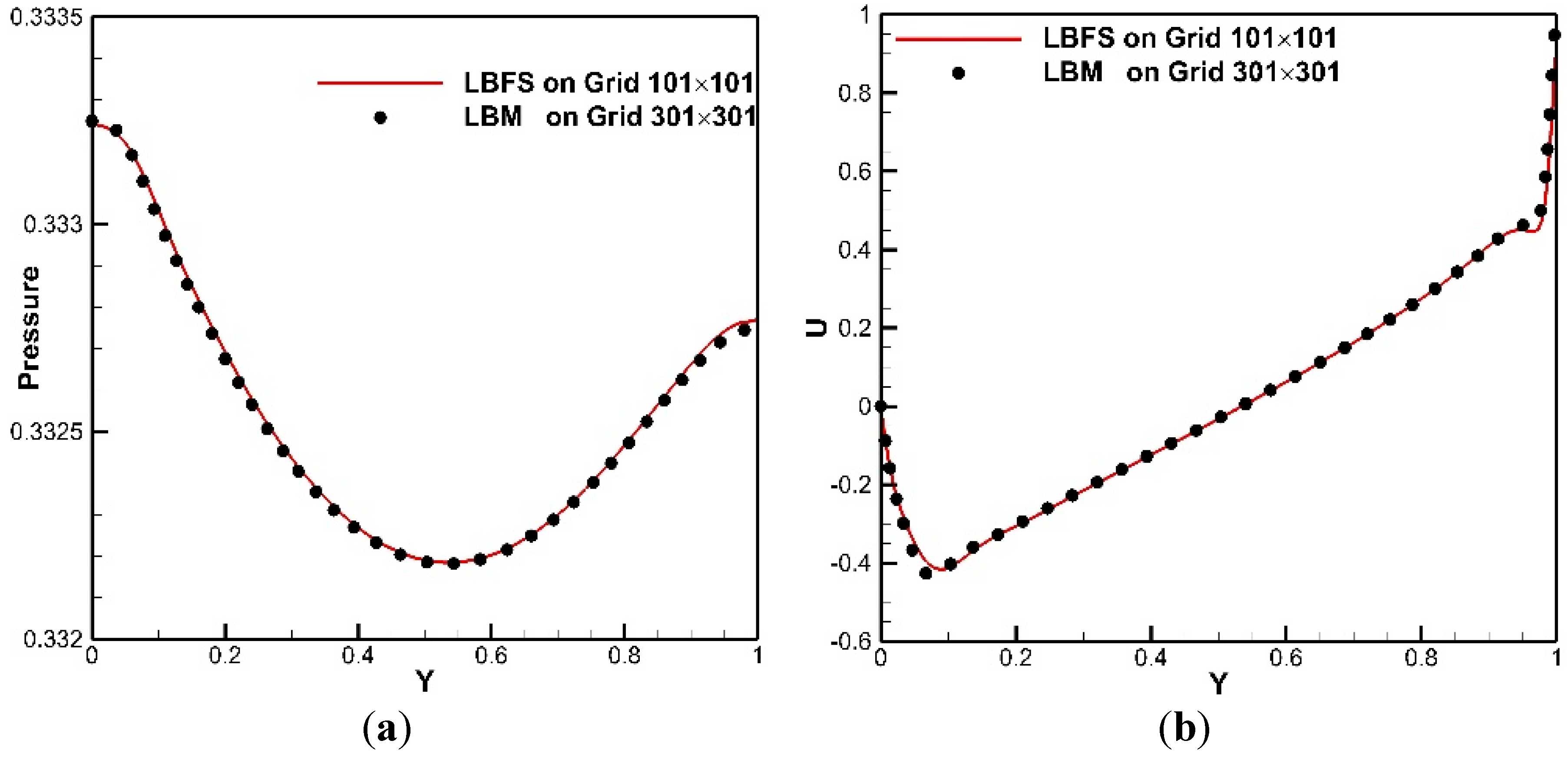
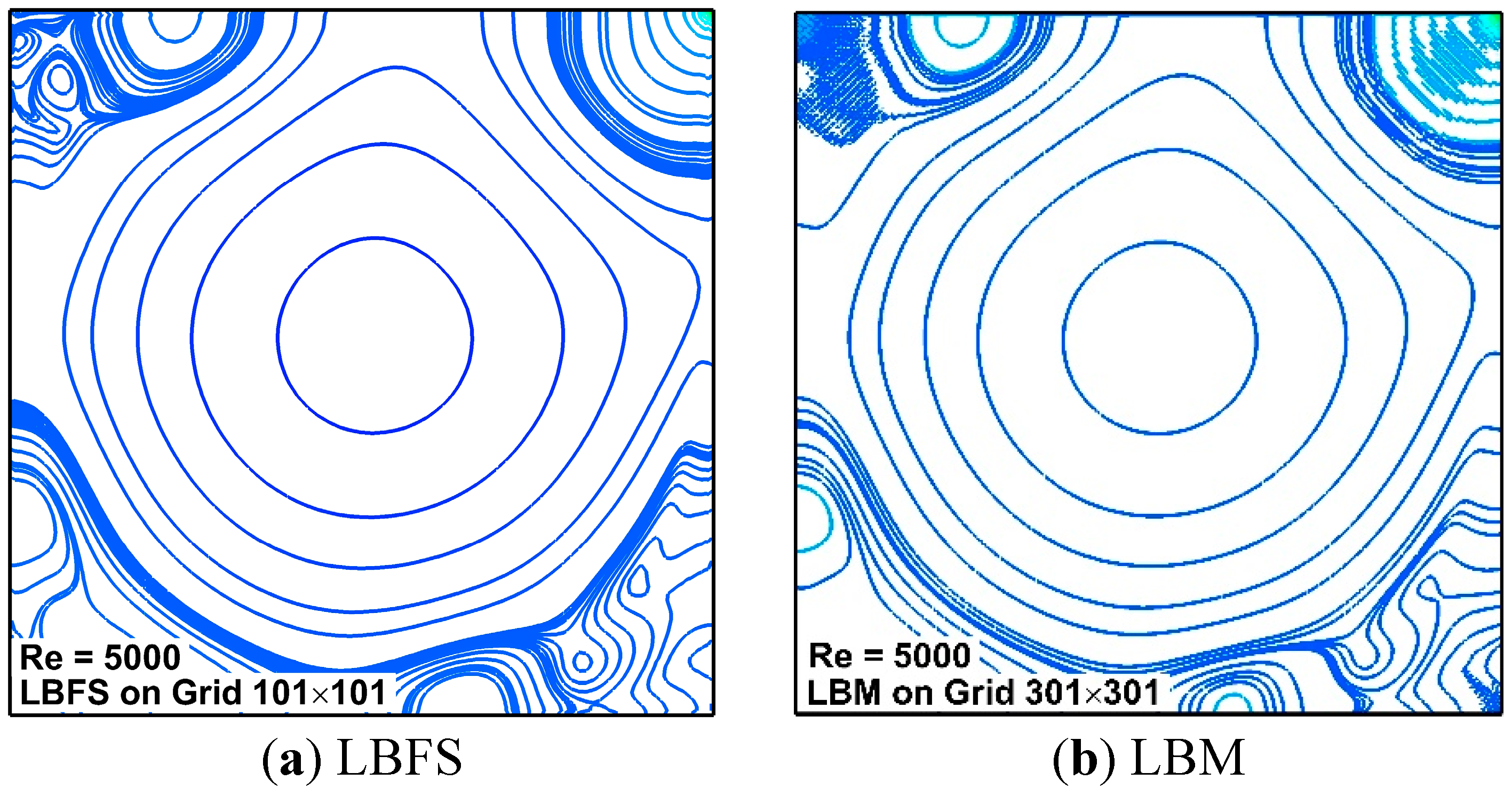
6.1. Lid-Driven Cavity Flows

As a benchmark problem, the classical lid-driven cavity flow has been studied extensively by many researchers [30,31,32,33,34]. This problem involves several geometrical and flow parameters: the length of the cavity $L$, the velocity of the lid $U$ and the density and dynamic viscosity of the fluid $\rho$ and $\mu$. With these parameters, the Reynolds number is defined as $\mathrm{Re}=\rho UL/\mu$. In present study, this problem will be solved by using the LBFS and the standard LBM to compare their accuracy, stability and efficiency in detail.

At first, the accuracy of the LBFS and LBM are examined by comparing the pressure and velocity profiles for lid-driven cavity flows at Re = 5000. In the computation, a non-uniform grid of $101\times 101$ for the LBFS and uniform grid of $301\times 301$ for LBM are applied. Note that much finer grid is required for the LBM to maintain numerical stability at this Reynolds number. Figure 4 compares the pressure and velocity profiles obtained by these two methods. It can be seen that excellent agreements have been achieved. Note that the LBFS uses about one-ninth of the total grid points adopted by the LBM, which shows its advantage and capability in applying non-uniform grids. It may also be noted that both LBFS and LBM have the second order of accuracy and quantitatively similar solutions will be obtained when the same grids are applied [8,9,10].

Figure 4. Comparison of pressure and velocity profiles on the vertical centerline for lid-driven cavity flows at Re = 5000. (a) Pressure; (b) Velocity.

Figure 4. Comparison of pressure and velocity profiles on the vertical centerline for lid-driven cavity flows at Re = 5000. (a) Pressure; (b) Velocity.

After that, the pure stability of the LBFS and LBM is investigated without considering numerical accuracy. This test is conducted by simulating the lid-driven cavity flows at Reynolds numbers from 100 to 5000. The minimum grids to get stable solution required respectively by the LBFS and LBM are recorded and shown in Table 1. It can be seen that, with the increase of Reynolds number, the LBM requires more grid points to maintain stability while the LBFS only needs a grid size of $4\times 4$ for all cases considered. This feature indicates that the LBFS is more stable than LBM. In addition, the stability of these two methods can be further examined by comparing numerical solutions for pressure. Figure 5 compares the pressure contours of lid-driven cavity flows at Reynolds number of 5000. A grid size of $101\times 101$ is applied by the LBFS and $301\times 301$ is applied by the LBM. It is obvious that the results of LBM for pressure field have substantial unphysical oscillations at the top left, top right and bottom right corners while those of the LBFS are smooth all over the flow domain. This phenomenon indicates that the stability of LBFS is superior to that of the LBM.

Table 1. Minimum required mesh resolution of the lattice Boltzmann flux solver (LBFS) and lattice Boltzmann method (LBM) for lid-driven cavity flows at different Reynolds numbers.

Re	100	1000	5000	7500
LBGK	5 × 5	39 × 39	219 × 219	341 × 341
LBFS	4 × 4	4 × 4	4 × 4	4 × 4

Table 1. Minimum required mesh resolution of the lattice Boltzmann flux solver (LBFS) and lattice Boltzmann method (LBM) for lid-driven cavity flows at different Reynolds numbers.

Re	100	1000	5000	7500
LBGK	5 × 5	39 × 39	219 × 219	341 × 341
LBFS	4 × 4	4 × 4	4 × 4	4 × 4

Figure 5. Comparison of pressure contours for lid-driven cavity flows at Re = 5000. (a) lattice Boltzmann flux solver (LBFS); (b) lattice Boltzmann method (LBM).

Figure 5. Comparison of pressure contours for lid-driven cavity flows at Re = 5000. (a) lattice Boltzmann flux solver (LBFS); (b) lattice Boltzmann method (LBM).

Moreover, the efficiency of the LBFS and LBM are investigated by considering two cases. The first one is their efficiency on the same uniform grid of $301\times 301$ by simulating the lid-driven cavity flow at Re = 5000. The other case is to examine the computational effort of the LBFS on non-uniform grids when its results agree well with those of the LBM. Table 2 compares the CPU time consumed by each solver in these two cases. As can be seen, when applied on the same grid, the LBFS takes about 3.8 times the computational time and 47% of the virtual memory that are required by the LBM. This is mainly attributed to the fact that, in the LBFS, interpolations of physical quantities are performed at each cell for flux reconstruction, which degrades its efficiency. On the other hand, when the solution of the LBFS compares well with that of LBM as shown in Figure 4, the LBFS only needs a non-uniform grid of $101\times 101$. As compared with those of LBM, only about 16.6% of computational time and 5.3% of virtual memory are consumed by the LBFS. This indicates that the LBFS needs less computational resources and can be more efficient for applications on non-uniform grids.

Table 2. Comparison of performance of the lattice Boltzmann flux solver (LBFS) and lattice Boltzmann method (LBM) on different grids for 2D lid-driven cavity flows at Re = 5000.

Object Type	Method	Min.	Max.	Avg.	Std. Dev.
Facility	V2SFCA	5	67	25.53	13.95
	EV2SFCA	5	118	27.71	23.88
Population	V2SFCA	5	63	23.20	15.08
	EV2SFCA	5	70	25.49	17.54

Table 2. Comparison of performance of the lattice Boltzmann flux solver (LBFS) and lattice Boltzmann method (LBM) on different grids for 2D lid-driven cavity flows at Re = 5000.

Object Type	Method	Min.	Max.	Avg.	Std. Dev.
Facility	V2SFCA	5	67	25.53	13.95
	EV2SFCA	5	118	27.71	23.88
Population	V2SFCA	5	63	23.20	15.08
	EV2SFCA	5	70	25.49	17.54

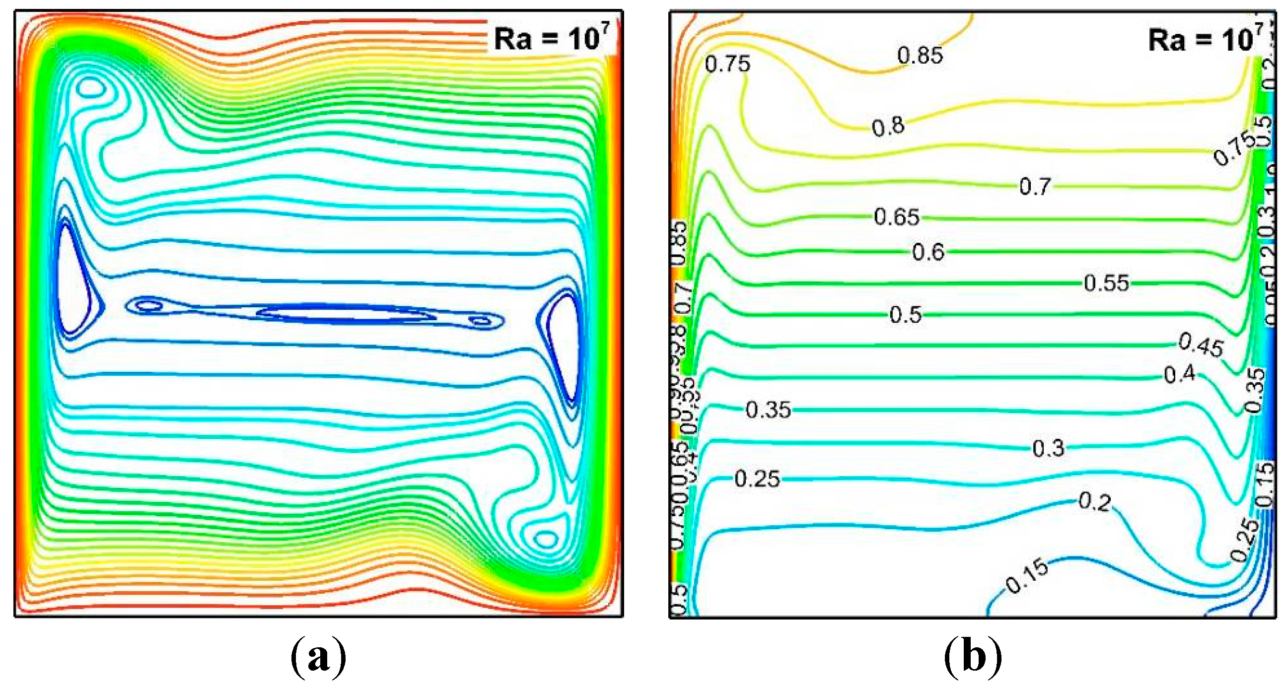
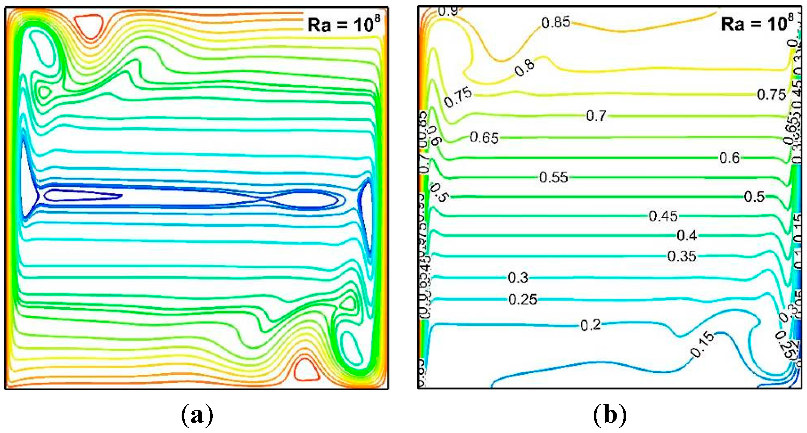
6.2. Natural Convection in a Square Cavity at High Rayleigh Number

Natural convection in a square cavity is a benchmark case for validating various numerical methods [35,37,42]. For instance, Peng et al. [42] simulated this problem at Rayleigh numbers from Ra = 10³ to 10⁶ to validate their simplified SRT-based thermal LB model. Guo et al. [37] studied this problem to examine their D2Q4 thermal LB model. Contrino et al. [35] validated their MRT-based thermal LB model by simulating this flow at high Rayleigh numbers of 10⁷ and 10⁸. Recently, with SRT-based D2Q9 thermal LB model, the LBFS [9] has also been validated through its application to simulate this problem from Ra = 10³ to 10⁶. It is noticed that, to study this problem, all versions of LBM restrict their computations on uniform grids. However, non-uniform grids may be more accurate and efficient to capture thin boundary layers, especially for flows at high Rayleigh numbers. This provides a good chance to examine the performance of the LBFS with D2Q4 thermal LB model.

The flow pattern of this problem is characterized by two normalized parameters: the Prandtl number $Pr$ and the Rayleigh number Ra, which can be respectively defined as:

$$Pr=\frac{\nu }{\chi }, Ra=\frac{g\beta \cdot \mathrm{\Delta }T\cdot L^3}{\nu \cdot \chi }=\frac{V_c^2\cdot L^2}{\nu \cdot \chi }$$

(36)

where $L$ is the length of the square cavity, $\mathrm{\Delta }T$ is the temperature difference between the hot and cold walls and $V_c=\sqrt{g\beta L\cdot \mathrm{\Delta }T}$ is the characteristic thermal velocity. The flow parameters are set as follows: $L=1$, $V_c=0.1$, Pr = 0.71. Two high Rayleigh numbers of $Ra={10}^7$ and 10⁸ are considered. Non-uniform grids with different grid sizes ($201\times 201$ and $301\times 301$ for $Ra={10}^7$; $301\times 301$ and $401\times 401$ for $Ra={10}^8$) are applied. To quantify the result, the mean Nusselt number $N{u}_{1/2}$ along the line of $x=L/2$ is computed and compared:

$$N{u}_{1/2}=\frac{L}{\chi \cdot \mathrm{\Delta }T}\cdot \frac{1}{L}{\displaystyle \underset{x=L/2}{\oint }\left(uT-\chi \frac{\partial T}{\partial x}\right)}dl$$

(37)

Table 3 and Table 4 show the maximum absolute value of the stream-function ${\left|\phi \right|}_{\max }$ and its position, the mean Nusselt number ${Nu}_{1/2}$ along the vertical centerline, the maximum u-velocity U_max along $x=L/2$ and its vertical position, the maximum v-velocity V_max along $y=L/2$ and its horizontal position. The numerical results of Contrino et al. [35] obtained by the MRT-LBM and those of Quere [43] obtained by a high order pseudo-spectral method are also included for comparison. With the increase of the grid size, the present solution is closer to the benchmark solution of Quere [43] for all cases considered. In particular, the relative error of ${\left|\phi \right|}_{\max }$ between the present solution on the finest grid and those of Quere [43] is within 0.26% and that of ${Nu}_{1/2}$ is within 0.08%. This indicates that both the strength of the flow field represented by the stream-function and the heat transfer rate represented by the mean Nusselt number are well predicted by the LBFS. Figure 6 and Figure 7 show the streamlines and isotherms at Rayleigh numbers of 10⁷ and 10⁸ respectively. At Ra = 10⁷, a large clock-wise recirculation is formed and attached to all walls. Both the flow and temperature boundary layers close to the hot and cold walls are very thin. The temperature at the same height of the cavity is almost a constant near central area. As Ra is increased to 10⁸, the boundary layer separates near the bottom left and top right region. Figure 8 shows the u-velocity along the vertical centerline and v-velocity along the horizontal centerline. As can be seen, the velocity component v is almost zero in a large zone except for those near the wall. This indicates that vertical convection in the central area can be very weak and heat conduction dominates this region. This is consistent with the observation that the temperature on the same latitude is almost a constant in the central area of the cavity.

Table 3. Comparison of representative quantities for natural convection in a square cavity at Ra = 10⁷.

Grid Size	Present		Contrino et al. [35]			Quere [43]
	2012	3012	3792	10192	15312
${\left|\phi \right|}_{\max }$	30.165	30.164	30.349	30.310	30.185	30.165
x	0.0868	0.0857	0.0848	0.0856	0.0857	0.86
y	0.5545	0.5559	0.5578	0.5562	0.5559	0.556
Nu1/2	16.550	16.543	16.526	16.523	16.523	16.52
Umax	148.17	148.84	148.48	148.57	148.58	148.59
y	0.8788	0.8789	0.8794	0.8793	0.8793	0.879
Vmax	699.19	699.91	699.11	699.27	699.31	699.18
x	0.0204	0.0216	0.0214	0.0213	0.0213	0.021

Table 3. Comparison of representative quantities for natural convection in a square cavity at Ra = 10⁷.

Grid Size	Present		Contrino et al. [35]			Quere [43]
	2012	3012	3792	10192	15312
${\left|\phi \right|}_{\max }$	30.165	30.164	30.349	30.310	30.185	30.165
x	0.0868	0.0857	0.0848	0.0856	0.0857	0.86
y	0.5545	0.5559	0.5578	0.5562	0.5559	0.556
Nu1/2	16.550	16.543	16.526	16.523	16.523	16.52
Umax	148.17	148.84	148.48	148.57	148.58	148.59
y	0.8788	0.8789	0.8794	0.8793	0.8793	0.879
Vmax	699.19	699.91	699.11	699.27	699.31	699.18
x	0.0204	0.0216	0.0214	0.0213	0.0213	0.021

Table 4. Comparison of representative quantities for natural convection in a square cavity at Ra = 10⁸.

Grid Size	Present		Contrino et al. [35]			Quere [43]
	301	4012	3792	10192	15312
${\left|\phi \right|}_{\max }$	53.955	53.893	54.870	54.106	53.953	53.85
x	0.0482	0.4760	0.0469	0.0478	0.0480	0.048
y	0.5536	0.5528	0.5594	0.5545	0.5533	0.553
Nu1/2	30.353	30.301	30.257	30.229	30.227	30.225
Umax	316.07	323.65	315.08	320.74	321.37	321.9
x	0.9267	0.9288	0.9239	0.9273	0.9276	0.928
Vmax	2221.1	2222.9	2221.4	2222.1	2222.3	2222
y	0.0118	0.1192	0.0121	0.0120	0.0120	0.012

Table 4. Comparison of representative quantities for natural convection in a square cavity at Ra = 10⁸.

Grid Size	Present		Contrino et al. [35]			Quere [43]
	301	4012	3792	10192	15312
${\left|\phi \right|}_{\max }$	53.955	53.893	54.870	54.106	53.953	53.85
x	0.0482	0.4760	0.0469	0.0478	0.0480	0.048
y	0.5536	0.5528	0.5594	0.5545	0.5533	0.553
Nu1/2	30.353	30.301	30.257	30.229	30.227	30.225
Umax	316.07	323.65	315.08	320.74	321.37	321.9
x	0.9267	0.9288	0.9239	0.9273	0.9276	0.928
Vmax	2221.1	2222.9	2221.4	2222.1	2222.3	2222
y	0.0118	0.1192	0.0121	0.0120	0.0120	0.012

Figure 6. Streamlines and isotherms for natural convection at Ra = 10⁷. (a) Streamlines; (b) Isotherms.

Figure 6. Streamlines and isotherms for natural convection at Ra = 10⁷. (a) Streamlines; (b) Isotherms.

Figure 7. Streamlines and isotherms for natural convection at Ra = 10⁸. (a) Streamlines; (b) Isotherms.

Figure 7. Streamlines and isotherms for natural convection at Ra = 10⁸. (a) Streamlines; (b) Isotherms.

Figure 8. Illustration of the velocity profiles at the centerlines for natural convection at Ra = 10⁷ and 10⁸. (a) Ra = 10⁷; (b) Ra = 10⁸.

Figure 8. Illustration of the velocity profiles at the centerlines for natural convection at Ra = 10⁷ and 10⁸. (a) Ra = 10⁷; (b) Ra = 10⁸.

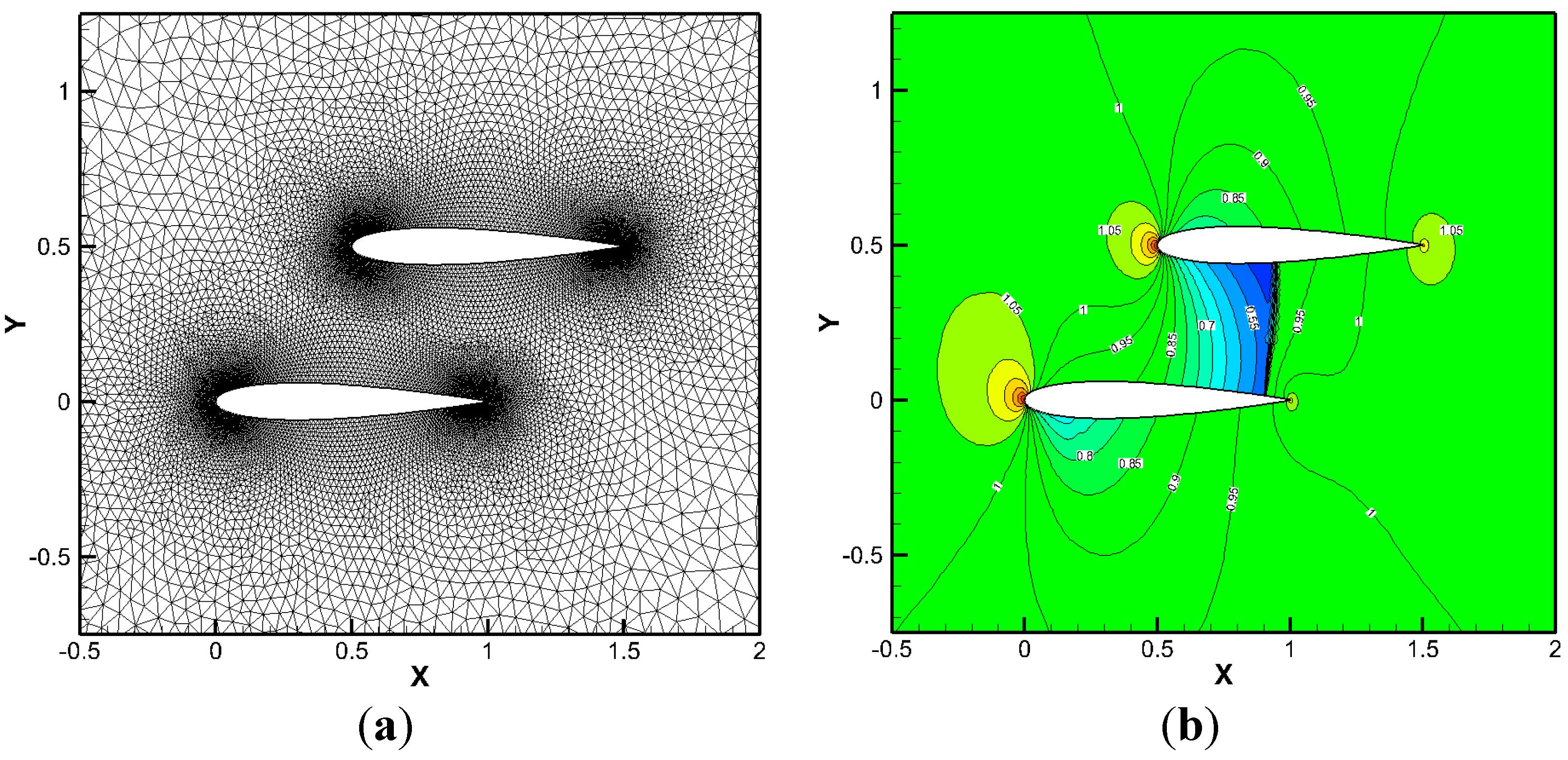
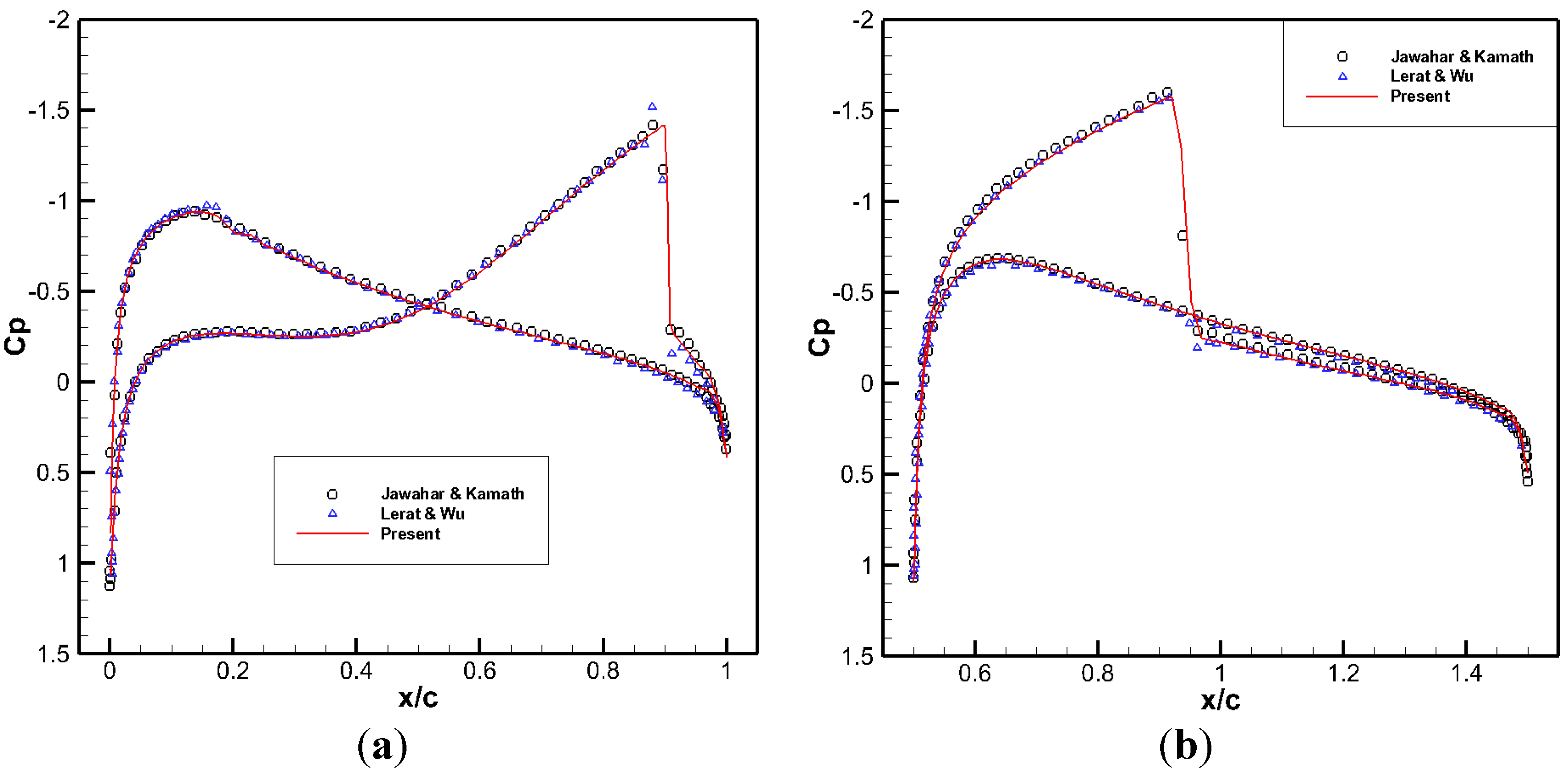
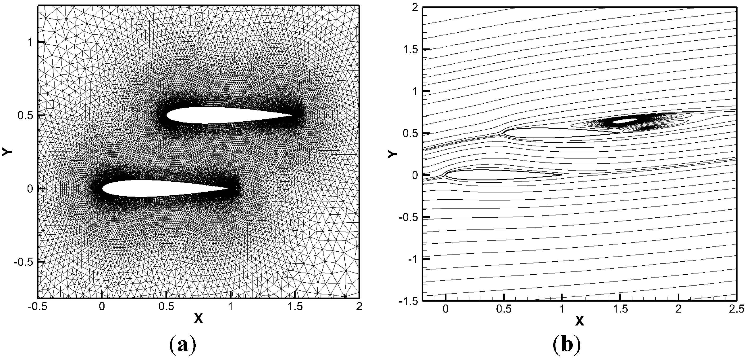
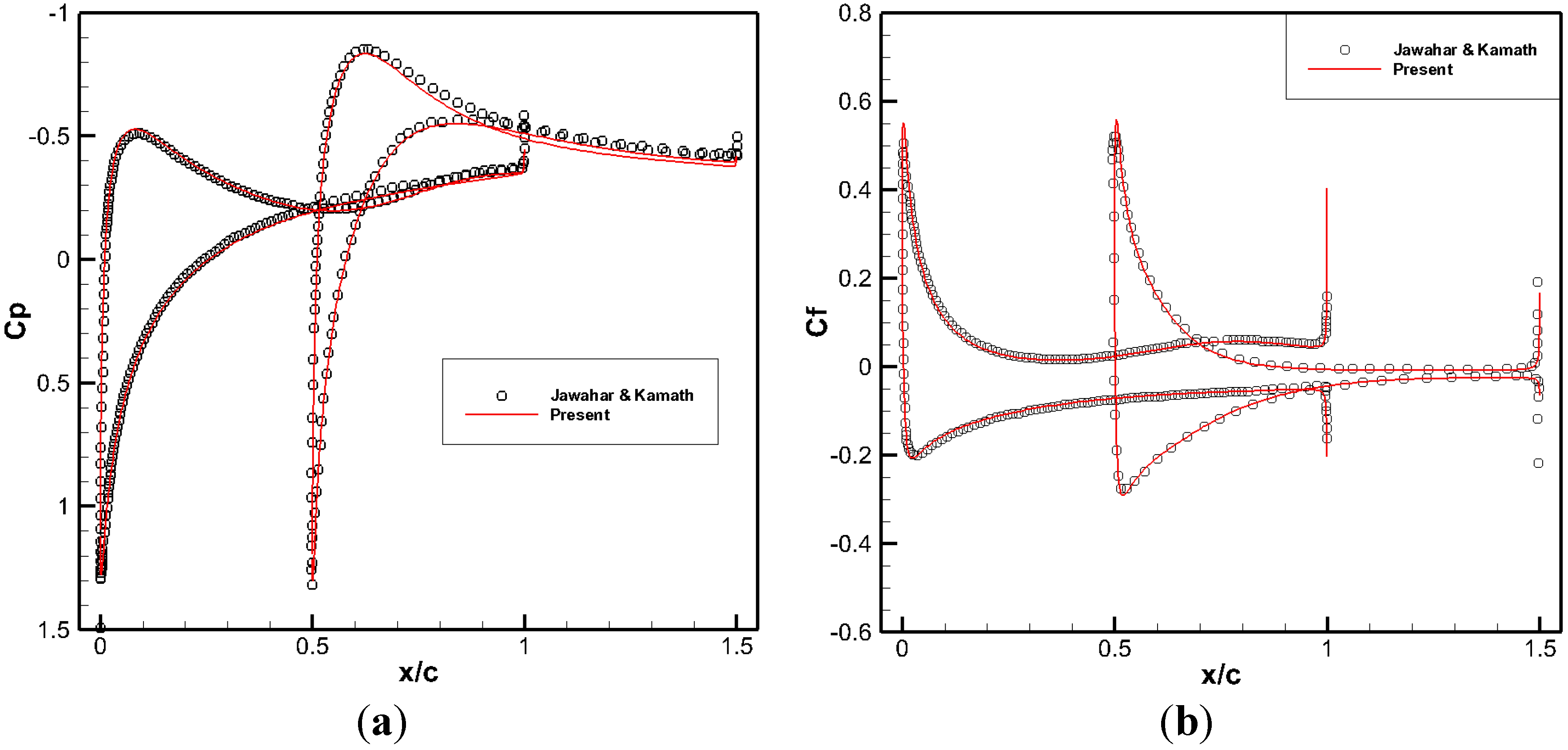
6.3. Inviscid and Viscous Transonic Flows Around a Staggered-Biplane Configuration

To validate the compressible LBFS for simulation of flows with complex geometry, the inviscid and viscous transonic flows around a staggered-biplane configuration are simulated. This test example is taken from the work of Jawahar and Kamath [44]. It comprises two NACA0012 airfoils, staggered by half a chord length in the pitchwise as well as chordwise directions. At first, the inviscid flow with the free-stream Mach number of 0.7 and the angle of attack of 0 degree is simulated. In the test, the unstructured grid containing 256 points on each airfoil and 36,727 triangular cells in the computational domain is utilized, and its partial view is shown in Figure 9a. The pressure contours obtained from present scheme are shown in Figure 9b. It can be seen from the figure that, a strong normal shock is formed between two airfoils and near the trailing edge of bottom airfoil, which is in line with those observed by Jawahar and Kamath [44] and Lerat and Wu [45]. Figure 10 shows the pressure coefficient distribution on the airfoil surface computed by present scheme. Also displayed in this figure are the results of Jawahar and Kamath [44] and Lerat and Wu [45]. Clearly, the results of current scheme agree well with the published data.

Figure 9. Partial view of computational mesh and pressure contours for inviscid biplane configuration. (a) Computational mesh; (b) Pressure contours.

Figure 9. Partial view of computational mesh and pressure contours for inviscid biplane configuration. (a) Computational mesh; (b) Pressure contours.

Figure 10. Comparison of pressure coefficient distribution on the surface of bottom and top airfoils for inviscid biplane configuration. (a) Bottom airfoil; (b) Top airfoil.

Figure 10. Comparison of pressure coefficient distribution on the surface of bottom and top airfoils for inviscid biplane configuration. (a) Bottom airfoil; (b) Top airfoil.

In addition, the viscous flow with the free-stream Mach number of 0.8, the Reynolds number of 500 and the angle of attack of 10 degree is simulated. In the simulation, the unstructured grid containing 512 points on each airfoil and 65,861 cells in the computational domain is used, and its partial view is shown in Figure 11a. Figure 11b shows the streamline pattern obtained from present scheme. From this figure, it can be observed that the separation region on the upper surface of top airfoil reveals two vortices. This observation is consistent with the results reported in [44]. As pointed out by Jawahar and Kamath [44], the secondary vortex is introduced by the bottom airfoil. The comparison of pressure coefficient and skin friction coefficient distributions on the airfoil surface obtained by present scheme with those reported in [44] is shown in Figure 12. Once again, the results obtained by present scheme compare well with the reference data.

Figure 11. Partial view of computational mesh and streamline pattern for viscous biplane configuration. (a) Computational mesh; (b) Streamline pattern.

Figure 11. Partial view of computational mesh and streamline pattern for viscous biplane configuration. (a) Computational mesh; (b) Streamline pattern.

Figure 12. Comparison of pressure coefficient and skin friction coefficient distributions for viscous biplane configuration. (a) Pressure coefficient distribution; (b) Skin friction distribution.

Figure 12. Comparison of pressure coefficient and skin friction coefficient distributions for viscous biplane configuration. (a) Pressure coefficient distribution; (b) Skin friction distribution.

7. Conclusions

As a finite-volume solver, the LBFS directly updates macroscopic flow variables at cell centers by solving macroscopic governing equations. Its fluxes are reconstructed locally at each interface through lattice moments of particle distribution functions, in which the relationships obtained from the Chapman–Enskog theory are applied. During local reconstruction, the LBM is applied locally in one streaming time step, which is different from the global application of the conventional LBM. As a consequence, the LBFS is able to combine the advantages of the finite volume method and the LBM.

In this work, the historic development from the LBM to the LBFS is briefly introduced and their relationships with the macroscopic conservation laws are also described through the multi-scale Chapman–Enksog analysis. The major contribution of this work is to refine and examine three different versions of the LBFS, proposed respectively for isothermal, thermal and compressible flows. In particular, the accuracy, stability and efficiency of the isothermal LBFS are compared with the LBM in detail. The LBFS for temperature field is simplified by the D2Q4 model, which reduces computational effort as compared with that by D2Q9 model. The LBFS for compressible flows is improved by incorporating non-equilibrium effects into the process for inviscid flux reconstruction, in which numerical dissipation can be controlled through a switch function.

Several benchmark problems, including lid-driven cavity flows, natural convection in a square cavity at high Rayleigh numbers of 10⁷ and 10⁸ and transonic flows around a staggered-biplane configuration, have been carried out to examine the solvers. Numerical results show that the LBFS is able to obtain comparable solutions with much less non-uniform grid points and its efficiency can be greatly improved. It is also shown that LBFS is much more stable than LBM and does not generate unphysical pressure oscillations for lid-driven cavity flows. With the application of one-dimensional compressible lattice Boltzmann model, the LBFS can be effectively applied for simulation of compressible flows on unstructured grids.

References

1. McNamara, G.R.; Zanetti, G. Use of the Boltzmann Equation to Simulate Lattice-Gas Automata. Phys. Rev. Lett. 1988, 61, 2332–2335. [Google Scholar] [CrossRef] [PubMed]
2. Higuera, F.J.; Succi, S.; Benzi, R. Lattice gas-dynamics with enhanced collisions. Europhys. Lett. 1989, 9, 345–349. [Google Scholar] [CrossRef]
3. Chen, S.Y.; Chen, H.D.; Martinez, D.; Matthaeus, W. Lattice Boltzmann model for simulation of magnetohydrodynamics. Phys. Rev. Lett. 1991, 67, 3776–3779. [Google Scholar] [CrossRef] [PubMed]
4. Qian, Y.H.; D’Humières, D.; Lallemand, P. Lattice BGK models for Navier–Stokes equation. Europhys. Lett. 1992, 17, 479–484. [Google Scholar] [CrossRef]
5. Mei, R.; Shyy, W. On the Finite Difference-Based Lattice Boltzmann Method in Curvilinear Coordinates. J. Comput. Phys. 1998, 143, 426–448. [Google Scholar] [CrossRef]
6. Hejranfar, K.; Ezzatneshan, E. Implementation of a high-order compact finite-difference lattice Boltzmann method in generalized curvilinear coordinates. J. Comput. Phys. 2014, 267, 28–49. [Google Scholar] [CrossRef]
7. Zarghami, A.; Ubertini, S.; Succi, S. Finite-volume lattice Boltzmann modeling of thermal transport in nanofluids. Comput. Fluids 2013, 77, 56–65. [Google Scholar] [CrossRef]
8. Wang, Y.; Shu, C.; Huang, H.B.; Teo, C.J. Multiphase lattice Boltzmann flux solver for incompressible multiphase flows with large density ratio. J. Comput. Phys. 2015, 280, 404–423. [Google Scholar] [CrossRef]
9. Wang, Y.; Shu, C.; Teo, C.J. Thermal lattice Boltzmann flux solver and its application for simulation of incompressible thermal flows. Comput. Fluids 2014, 94, 98–111. [Google Scholar] [CrossRef]
10. Shu, C.; Wang, Y.; Teo, C.J.; Wu, J. Development of Lattice Boltzmann Flux Solver for Simulation of Incompressible Flows. Adv. Appl. Math. Mech. 2014, 6, 436–460. [Google Scholar]
11. Yang, L.M.; Shu, C.; Wu, J. A moment conservation-based non-free parameter compressible lattice Boltzmann model and its application for flux evaluation at cell interface. Comput. Fluids 2013, 79, 190–199. [Google Scholar] [CrossRef]
12. Guo, Z.; Shi, B.; Wang, N. Lattice BGK Model for Incompressible Navier–Stokes Equation. J. Comput. Phys. 2000, 165, 288–306. [Google Scholar] [CrossRef]
13. Shan, X.; Chen, H. Lattice Boltzmann model for simulating flows with multiple phases and components. Phys. Rev. E 1993, 47, 1815–1819. [Google Scholar] [CrossRef]
14. Lee, T.; Lin, C.-L. A stable discretization of the lattice Boltzmann equation for simulation of incompressible two-phase flows at high density ratio. J. Comput. Phys. 2005, 206, 16–47. [Google Scholar] [CrossRef]
15. He, X.; Chen, S.; Zhang, R. A Lattice Boltzmann Scheme for Incompressible Multiphase Flow and Its Application in Simulation of Rayleigh–Taylor Instability. J. Comput. Phys. 1999, 152, 642–663. [Google Scholar] [CrossRef]
16. Li, Q.; He, Y.L.; Wang, Y.; Tao, W.Q. Coupled double-distribution-function lattice Boltzmann method for the compressible Navier–Stokes equations. Phys. Rev. E 2007, 76, 056705. [Google Scholar] [CrossRef] [PubMed]
17. Chen, F.; Xu, A.; Zhang, G.; Li, Y.; Succi, S. Multiple-relaxation-time lattice Boltzmann approach to compressible flows with flexible specific-heat ratio and Prandtl number. Europhys. Lett. 2010, 90. [Google Scholar] [CrossRef]
18. He, Y.-L.; Liu, Q.; Li, Q. Three-dimensional finite-difference lattice Boltzmann model and its application to inviscid compressible flows with shock waves. Physica A 2013, 392, 4884–4896. [Google Scholar] [CrossRef]
19. Nie, X.; Doolen, G.D.; Chen, S. Lattice-Boltzmann Simulations of Fluid Flows in MEMS. J. Stat. Phys. 2002, 107, 279–289. [Google Scholar] [CrossRef]
20. Lim, C.Y.; Shu, C.; Niu, X.D.; Chew, Y.T. Application of lattice Boltzmann method to simulate microchannel flows. Phys. Fluids 2002, 14, 2299–2308. [Google Scholar] [CrossRef]
21. Meng, J.; Zhang, Y. Accuracy analysis of high-order lattice Boltzmann models for rarefied gas flows. J. Comput. Phys. 2011, 230, 835–849. [Google Scholar] [CrossRef] [Green Version]
22. Lallemand, P.; Luo, L.-S. Theory of the lattice Boltzmann method: Dispersion, dissipation, isotropy, Galilean invariance, and stability. Phys. Rev. E 2000, 61, 6546–6562. [Google Scholar] [CrossRef]
23. Niu, X.D.; Shu, C.; Chew, Y.T. A lattice Boltzmann BGK model for simulation of micro flows. Europhys. Lett. 2004, 67, 600–606. [Google Scholar] [CrossRef]
24. Yuan, H.-Z.; Niu, X.-D.; Shu, S.; Li, M.; Yamaguchi, H. A momentum exchange-based immersed boundary-lattice Boltzmann method for simulating a flexible filament in an incompressible flow. Comput. Math. Appl. 2014, 67, 1039–1056. [Google Scholar] [CrossRef]
25. Yuan, H.-Z.; Shu, S.; Niu, X.-D.; Li, M.; Hu, Y. A Numerical Study of Jet Propulsion of an Oblate Jelly fish Using a Momentum Exchange-Based Immersed Boundary-Lattice Boltzmann Method. Adv. Appl. Math. Mech. 2014, 6, 307–326. [Google Scholar]
26. Ubertini, S.; Succi, S. Recent advances of Lattice Boltzmann techniques on unstructured grids. Prog. Comput. Fluid Dyn. Int. J. 2005, 5, 85–96. [Google Scholar] [CrossRef]
27. Rossi, N.; Ubertini, S.; Bella, G.; Succi, S. Unstructured lattice Boltzmann method in three dimensions. Int. J. Numer. Methods Fluids 2005, 49, 619–633. [Google Scholar] [CrossRef]
28. Patankar, S.V.; Spalding, D.B. A calculation procedure for heat, mass and momentum transfer in three-dimensional parabolic flows. Int. J. Heat Mass Transf. 1972, 15, 1787–1806. [Google Scholar] [CrossRef]
29. Sun, D.L.; Qu, Z.G.; He, Y.L.; Tao, W.Q. An efficient segregated algorithm for incompressible fluid flow and heat transfer problems-IDEAL (Inner Doubly Iterative Efficient Algorithm for Linked Equations) Part I: Mathematical formulation and solution procedure. Numer. Heat Transf. B 2008, 53. [Google Scholar] [CrossRef]
30. Bruneau, C.-H.; Saad, M. The 2D lid-driven cavity problem revisited. Comput. Fluids 2006, 35, 326–348. [Google Scholar] [CrossRef]
31. Kalita, J.C.; Gupta, M.M. A streamfunction–velocity approach for 2D transient incompressible viscous flows. Int. J. Numer. Methods Fluids 2010, 62, 237–266. [Google Scholar] [CrossRef]
32. Lin, L.-S.; Chang, H.-W.; Lin, C.-A. Multi relaxation time lattice Boltzmann simulations of transition in deep 2D lid driven cavity using GPU. Comput. Fluids 2013, 80, 381–387. [Google Scholar] [CrossRef]
33. Zhuo, C.; Zhong, C.; Cao, J. Filter-matrix lattice Boltzmann simulation of lid-driven deep-cavity flows, Part I—Steady flows. Comput. Math. Appl. 2013, 65, 1863–1882. [Google Scholar] [CrossRef]
34. Zhuo, C.; Zhong, C.; Cao, J. Filter-matrix lattice Boltzmann simulation of lid-driven deep-cavity flows, Part II—Flow bifurcation. Comput. Math. Appl. 2013, 65, 1883–1893. [Google Scholar] [CrossRef]
35. Contrino, D.; Lallemand, P.; Asinari, P.; Luo, L.-S. Lattice-Boltzmann simulations of the thermally driven 2D square cavity at high Rayleigh numbers. J. Comput. Phys. 2014, 275, 257–272. [Google Scholar] [CrossRef]
36. Luan, H.-B.; Xu, H.; Chen, L.; Sun, D.-L.; He, Y.-L.; Tao, W.-Q. Evaluation of the coupling scheme of FVM and LBM for fluid flows around complex geometries. Int. J. Heat Mass Transf. 2011, 54, 1975–1985. [Google Scholar] [CrossRef]
37. Guo, Z.; Shi, B.; Zheng, C. A coupled lattice BGK model for the Boussinesq equations. Int. J. Numer. Methods Fluids 2002, 39, 325–342. [Google Scholar] [CrossRef]
38. Chen, L.; He, Y.-L.; Kang, Q.; Tao, W.-Q. Coupled numerical approach combining finite volume and lattice Boltzmann methods for multi-scale multi-physicochemical processes. J. Comput. Phys. 2013, 255, 83–105. [Google Scholar] [CrossRef]
39. Chen, L.; Luan, H.; Feng, Y.; Song, C.; He, Y.-L.; Tao, W.-Q. Coupling between finite volume method and lattice Boltzmann method and its application to fluid flow and mass transport in proton exchange membrane fuel cell. Int. J. Heat Mass Transf. 2012, 55, 3834–3848. [Google Scholar] [CrossRef]
40. Yang, L.M.; Shu, C.; Wu, J.; Zhao, N.; Lu, Z.L. Circular function-based gas-kinetic scheme for simulation of inviscid compressible flows. J. Comput. Phys. 2013, 255, 540–557. [Google Scholar] [CrossRef]
41. Yang, L.M.; Shu, C.; Wu, J. A three-dimensional explicit sphere function-based gas-kinetic flux solver for simulation of inviscid compressible flows. J. Comput. Phys. 2015, 295, 322–339. [Google Scholar] [CrossRef]
42. Peng, Y.; Shu, C.; Chew, Y.T. Simplified thermal lattice Boltzmann model for incompressible thermal flows. Phys. Rev. E 2003, 68, 026701. [Google Scholar] [CrossRef] [PubMed]
43. Le Quéré, P. Accurate solutions to the square thermally driven cavity at high Rayleigh number. Comput. Fluids 1991, 20, 29–41. [Google Scholar] [CrossRef]
44. Jawahar, P.; Kamath, H. A High-Resolution Procedure for Euler and Navier–Stokes Computations on Unstructured Grids. J. Comput. Phys. 2000, 164, 165–203. [Google Scholar] [CrossRef]
45. Lerat, A.; Wu, Z.N. Stable Conservative Multidomain Treatments for Implicit Euler Solvers. J. Comput. Phys. 1996, 123, 45–64. [Google Scholar] [CrossRef]