Article

Identify the Rotating Stall in Centrifugal Compressors by Fractal Dimension in Reconstructed Phase Space

School of Energy and Power Engineering, Xi’an Jiaotong University, 710049 Xi’an, China
*
Author to whom correspondence should be addressed.
Entropy 2015, 17(12), 7888-7899; https://0-doi-org.brum.beds.ac.uk/10.3390/e17127848
Submission received: 28 August 2015 / Revised: 26 October 2015 / Accepted: 16 November 2015 / Published: 30 November 2015
(This article belongs to the Special Issue Complex and Fractional Dynamics)

Abstract

:
Based on phase space reconstruction and fractal dynamics in nonlinear dynamics, a method is proposed to extract and analyze the dynamics of the rotating stall in the impeller of centrifugal compressor, and some numerical examples are given to verify the results as well. First, the rotating stall of an existing low speed centrifugal compressor (LSCC) is numerically simulated, and the time series of pressure in the rotating stall is obtained at various locations near the impeller outlet. Then, the phase space reconstruction is applied to these pressure time series, and a low-dimensional dynamical system, which the dynamics properties are included in, is reconstructed. In phase space reconstruction, C–C method is used to obtain the key parameters, such as time delay and the embedding dimension of the reconstructed phase space. Further, the fractal characteristics of the rotating stall are analyzed in detail, and the fractal dimensions are given for some examples to measure the complexity of the flow in the post-rotating stall. The results show that the fractal structures could reveal the intrinsic dynamics of the rotating stall flow and could be considered as a characteristic to identify the rotating stall.

1. Introduction

The centrifugal compressor is a mechanical device used to enhance the static pressure of a compressible fluid, and it is widely used in energy and power engineering, such as some uses of centrifugal compression systems including reaction processes in chemical industries, compression and transportation of hydrogen in petrochemical refineries, refrigeration systems that contain heat pumps powered by small centrifugal compressors, etc. However, the efficiency and stability of a centrifugal compressor are restricted by the phenomena of the rotating stall and surge. It is one of the primary problems to be improved: the compressor aerodynamic performance by controlling the rotating stall. Hence, the studies of dynamical characteristics of the rotating stall and the flow inside the compressor impeller are important in the control of the rotating stall.
At present, the spectra analysis for fluctuating pressure which is obtained by some fixed probes in the rotating stall is the main method for extracting the characteristics of system, and the flow is controlled by injection air, namely, active control. Specifically, stall and flow separation of centrifugal compressors are studied with numerical simulation, and the method of injection air is used to modify the local flow near the blade leading edges, in order to suppress the rotating stall and surge [1,2,3]. Furthermore, the rotating stall of the axial compressor is studied with an experimental method, and it is found that the stall cell blockage is an important parameter or factor for correlating the flow regimes in stall and the overall compressor performance [4,5,6]. The flow instability in compressor has been studied by other researchers [7,8,9,10], but little research on the rotating stalls are studied with dynamics.
Because of the complexity and nonlinear characteristics of the flow field in the rotating stall, such as aperiodicity, discontinuity and transition, a new method is developed to study the complex flow field of static and dynamic stalls on the basis of theory of nonlinear dynamics, especially the chaos and fractal theories [11,12]. The rotating stall in the centrifugal compressor in the general case is analyzed by an observation variable of the system which is a time series considered as a dynamic system, but the dynamic characteristics which are hidden in system cannot be shown directly by studying the time series of such state variables. Using the phase space reconstruction in nonlinear dynamics theory, the characteristics of dynamics can be drawn from the time series of single variables, and can be used as a measure for identifying the rotating stall. Indeed, the identification of the intrinsic characteristics in the rotating stall is a new way to control the rotating stall in advance.
The phase space reconstruction for time series was proposed in 1980 [13], and then this method is extended to more fields by some other researchers, in combination with other techniques [14,15]. For example, the chaotic attractor is used to predict the rotating stall of the compressor [16]. In addition, a comparative study about the correlation dimension of the pressure signal in pre- and post- stall is given, and the correlation dimension can be considered as an intrinsic characteristic of the stall in a fan [17].
In this paper, based on the numerical simulation of the flow in centrifugal impeller in the pre- and post- rotating stall, the pressure time series are studied by phase space reconstruction with the C–C method. Then, the fractal structure is found from the pressure time series in the rotating stall, and the fractal dimension is given to describe the complexity in fractal structure. In a sense, the fractal structure can be considered as a dynamics characteristics of the rotating stall in centrifugal impeller, and there is significance in guiding to identify the rotating stall in accuracy. Finally, the pressure time series, which are sampled at different locations near the impeller outlet as the rotating stall, are studied by phase space reconstruction, and their fractal dimension is calculated, respectively.

2. Numerical Simulations of the Rotating Stall in the Centrifugal Impeller

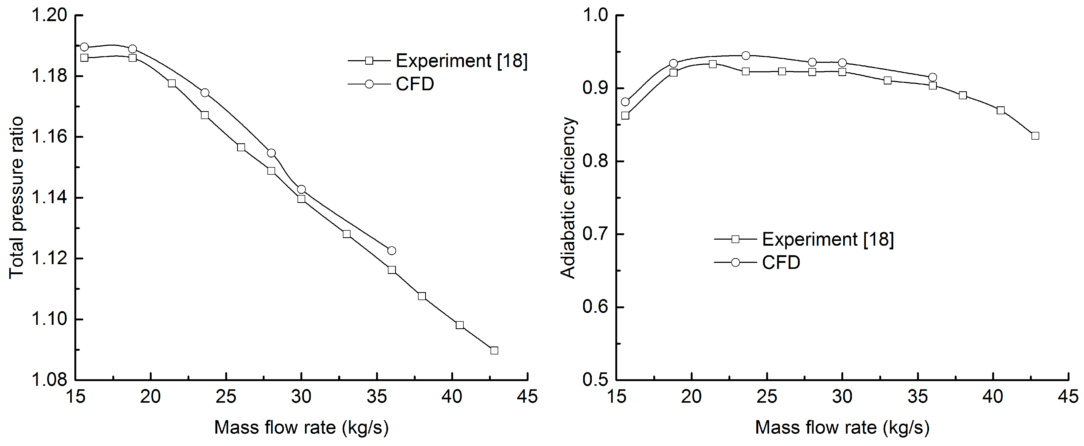
2.1. The Model and Numerical Method

In this paper, a NASA (National Aeronautics and Space Administration) low-speed centrifugal impeller (LSCC), which is a classic example with some experimental results, is used as a benchmark for numerical example and verification. The impeller has 20 back curved blades with the outlet angle of 55°. The diameter of impeller entrance is 870 mm, the blade height 218 mm, the outlet diameter 1524 mm, the blade height 141 mm, the impeller blade tip clearance constant 2.54 mm. Furthermore, the specification speed is 1862 r/min, the pressure 1 atm, the temperature 25 °C, flow rate 30 kg/s, pressure ratio 1.141, and the efficiency 92.2% [18].
Numerical simulations are carried out to obtain the information at the compressor the rotating stall condition. The numerical mode uses a full 360° model which contains the 3-D impeller, the inlet region and the part of diffuser. The computational domain is divided into unstructured grid by the Gambit, the grid number is about 2.98 million, and there are few changes in the results of numerical simulations with the grid refinement. The flow region in impeller is set as rotate region, the inlet region and diffuser are set as the fix region, and the interface boundary condition is used between the rotate and the fix region. The flow field is simulated by commercial software Fluent, which uses the SIMPLE method to solve the three dimensional compressible Reynolds averaged Navier–Stokes equations, and the working medium is ideal gas. In addition, the steady calculation is run to verify the results of the numerical and the experimental, and the unsteady calculation is run when the flow decreases to 12.6 kg/s.
The comparisons between the numerical and the experimental results is shown in Figure 1. There is quite a good agreement between the numerical and experimental results even if it is somehow higher than the experimental results.
Figure 1. Performance comparisons between the numerical and the experimental results.
Entropy 17 07848 g001

2.2. The Model and Numerical Method

Figure 2a–c shows the pressure profiles as the flow rates are 30 kg/s, 23.6 kg/s and 12.6 kg/s at 42.8% blade height, respectively.
Figure 2. (a) Pressure distribution as the flow rates is 30 kg/s at 42.8% blade height; (b) pressure distribution as the flow rates is 23.6 kg/s at 42.8% blade height; (c) pressure distribution as the flow rates is 12.6 kg/s at 42.8% blade height.
Entropy 17 07848 g002
From Figure 2, it is clear that the impeller works well as the flow rate is 30 kg/s, because it is at design condition. When the flow decreases to 23.6 kg/s [18], the pressure at outlet increases and the compressor runs efficiently. When the flow decreases to 12.6 kg/s, the local high pressure area appears near the inlet of flow passages, implying that the normal flow is blocked by such cells with local high pressure. As a result, the pressure at the impeller outlet drops sharply. That is, the stability of flow is lost, and the compressor is working in the rotating stall.

3. Phase Space Reconstruction of Pressure Time Series

3.1. Phase Space Reconstruction
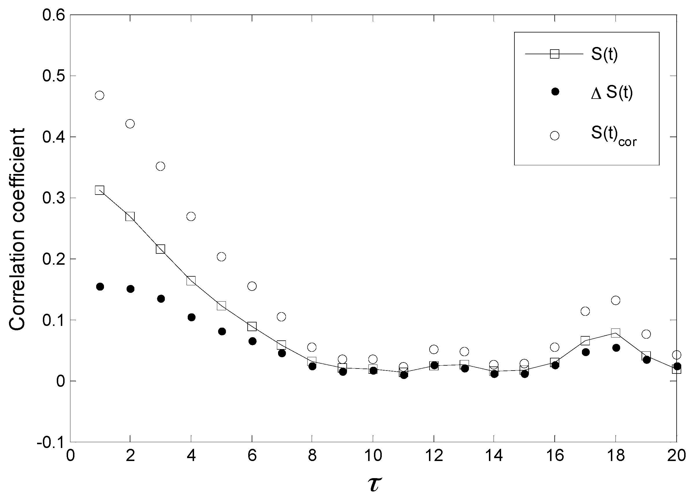
The derivative recovery method is the simplest one for phase space reconstruction with time series. However, in practical application, the information of time series cannot be known in advance, so the derivative operation is influenced greatly by the operating error. As a result, the reliability of phase space analysis becomes weak. Therefore, the time delay method is proposed for phase space reconstruction by Takens, and the essence of this method is to construct the m dimensional phase space by different time delay τ , with one dimensional time series { x ( n ) } as following,
X ( i ) = { x ( i ) , x ( i + τ ) , , x ( i + ( m 1 ) τ ) }
The conditions in which the topological equivalence between the reconstructed phase space and the original dynamic system should be satisfied. Moreover, the dynamics characteristics of the system will be shown by the phase portrait of the reconstructed pressure time series. As the phase portrait of reconstructed phase space presents some special or singular structures (e.g., fractal attractor), it implies that there are chaotic characteristics in the system [19].
There are two key parameters used to reconstruct the phase space as the method of time delay is applied, namely, embedding dimension m and the time delay τ , and these two parameters can be set by any value if the chaotic time series is infinitely long and makes no noise, following Takens theorem. However, in the application, none of these time series can be infinite and have no noise, so the embedding dimension and time delay cannot be determined exactly following theorem.
To this end, the correlation integral and its calculation formulas are proposed based on the time delay method to reconstruct the phase space by Grasssberger and Procaccia [20], and they can be applied to calculate the dimension of chaotic attractor, and hence this method is called the G–P algorithm. Further, the C–C method, a method which is much more commonly used in practice based on the correlation integral calculation, is proposed and used to calculate the embedding dimension and the time delay in this paper. A brief introduction will be given in the following.

3.2. C–C Method

The length of the time window is proposed by Kugiumtzis [21]. Following his method, the selection of time delay cannot be independent on embedding dimension, but it depends on the length of the time window. Further, Kim et al. proposed the C–C method based on the length of time window [22].
Suppose that the sampling interval of the time series is τ s , the optimal time of delay time series τ d = t τ s , the embedding dimension m , the time delay window τ w , N the size of the data, the number of data points M = N ( m 1 ) τ , the time delay τ ( τ = t ) , and then the correlation integral of reconstructed phase space with embedding time series can be obtained as following,
C ( m , N , r , t ) = 2 M ( M 1 ) 1 i j M θ ( r d i j )
In fact, the correlation integral is the probability of the distance between any two points as it is less than r .
Defining the statistics as
S ( m , N , r , t ) = C ( m , N , r , t ) C m ( 1 , N , r , t )
In application, the time series will be divided into t groups disjointing sub-sequences with length N s = N / t , the time delay of phase space reconstruction is t,
{ x 1 , x t + 1 , , x N t + 1 } { x 2 , x t + 2 , , x N t + 2 } { x t , x 2 t , , x N }
Then, defining each sequence of S ( m , N , r , t ) as
S ( m , N , r , t ) = 1 t s = 1 t [ C s ( m , N t , r , t ) C s m ( 1 , N t , r , t ) ]
When N ,
S ( m , r , t ) = 1 t s = 1 t [ C s ( m , r , t ) C s m ( 1 , r , t ) ]
where m = 2 , 3 , .
If each sub-sequence is independent identical distribution, as the embedding dimension and time delay are fixed, then the values of S ( m , r , t ) is zero. However, in actuality, time series are correlated to time, so the values of S ( m , r , t ) is non-zero. The autocorrelation of time series is embodied by S ( m , r , t ) ~ t , and the first value of S ( m , r , t ) ~ t is the optimal time delay τ d . In this case, the point’s distribution of phase space reconstruction is approximately uniform distribution, and the attractor structure in reconstruction will be unfolded fully in the phase space.
Defining the radius difference of maximum and minimum as
Δ S ( m , t ) = max { S ( m , r j , t ) } min { S ( m , r j , t ) }
where S ( m , r , t ) ~ t is the maximum deviation of entire radius, the optimal time delay τ d should be chosen as the value of the first local minimum of Δ S ( m , t ) .
In C–C method, when 2 m 5 , σ / 2 r 2 σ , N 500 , the correlation of time series will be shown well in S ( m , N , r , 1 ) . Among them, σ is standard deviation or mean-square deviation of the time series.
From the estimation N , m , r , taking m = 2 ,   3 ,   4 ,   5 , r i = i σ / 2 , i = 1 , 2 , 3 , 4 , yields,
S ¯ ( t ) = 1 16 m = 2 5 j = 1 4 S ( m , r j , t )
Δ S ¯ ( t ) = 1 4 m = 2 5 Δ S ( m , t )
S c o r ( t ) = Δ S ¯ ( t ) + | S ¯ ( t ) |
The optimal time delay of time series τ d is chosen as the first value of S ¯ ( t ) or the first local minimum of Δ S ¯ ( t ) , and the time window τ w is chosen as global minimum of S c o r ( t ) , and τ w = ( m 1 ) τ .

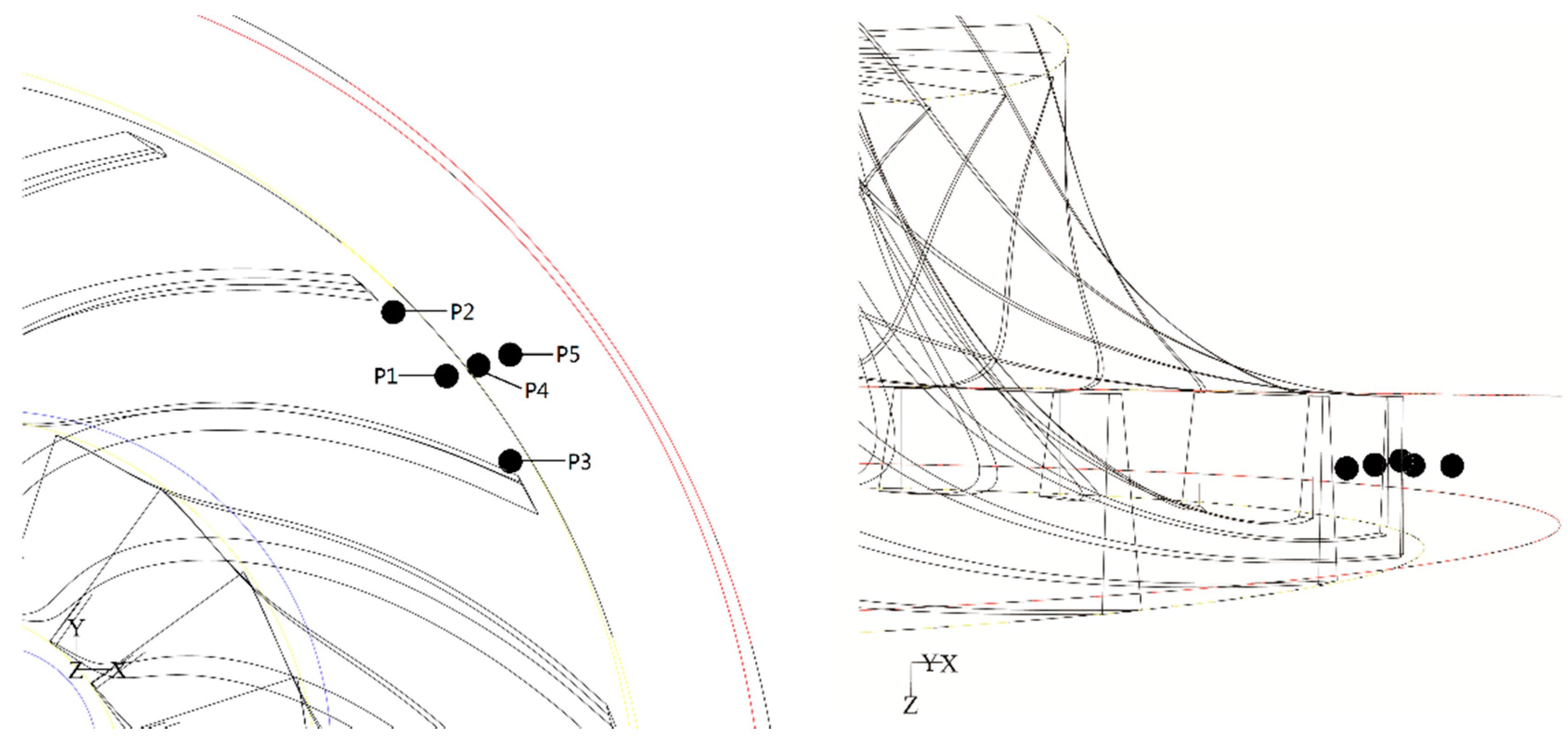
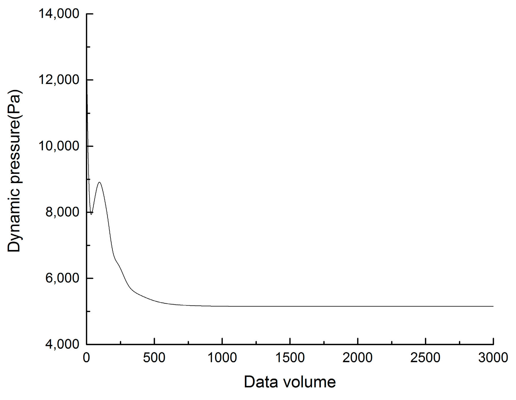
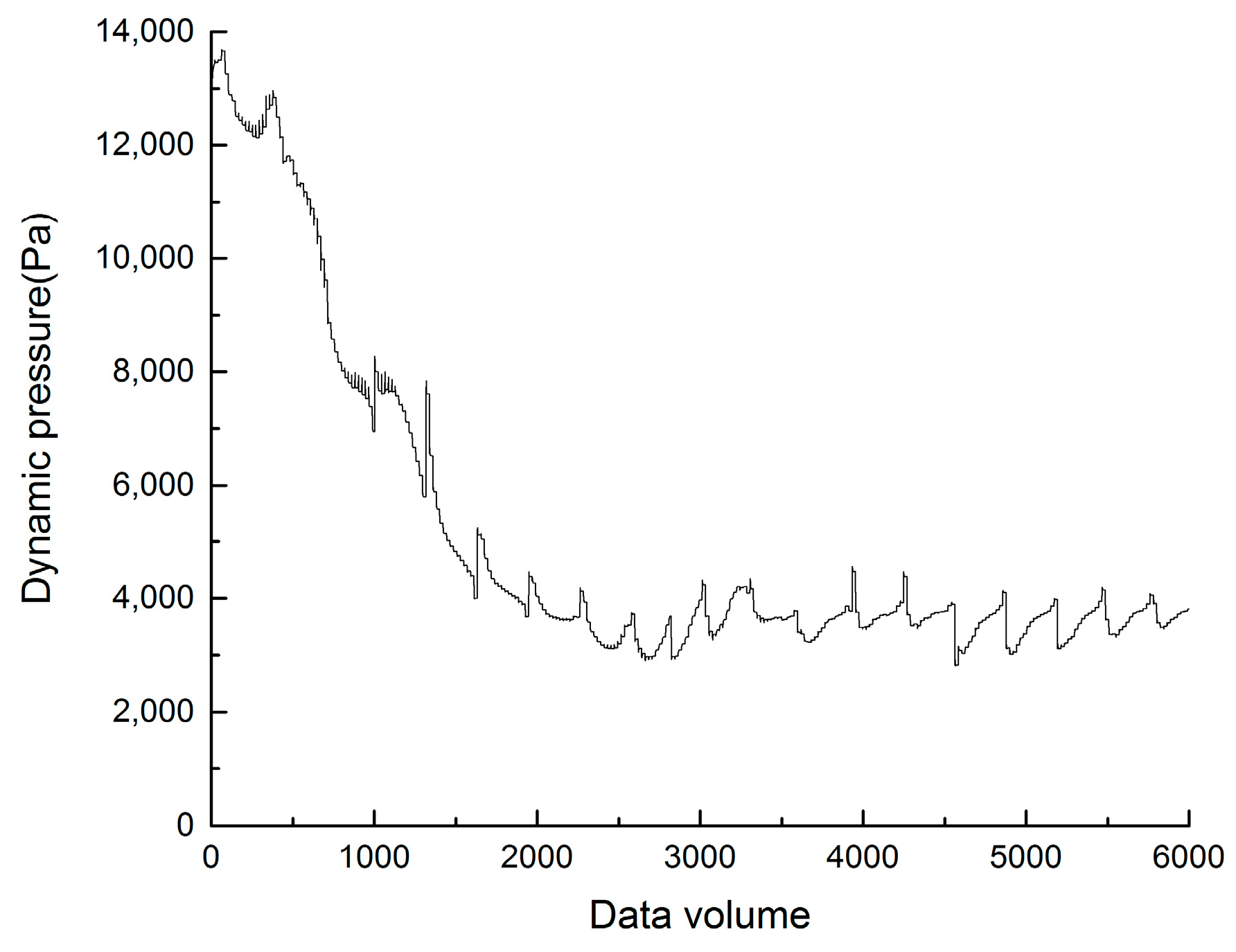
3.3. Pressure Time Series of the Sampling Points

Figure 3 shows the locations of sampling points for sampling the pressure time series in the pre- and post- rotating stall.
In this paper, P1–P5 are five fixed sampling points. Firstly, the pressure time series at P1 in the pre- and post- rotating stall are analyzed by phase space reconstruction. Furthermore, the phase space reconstructions of the pressure time series at P2, P3, P4 and P5 in pre- and post- rotating stall are studied and compared with each other, respectively.
Figure 3. Sampling points of the pressure time series.
Entropy 17 07848 g003

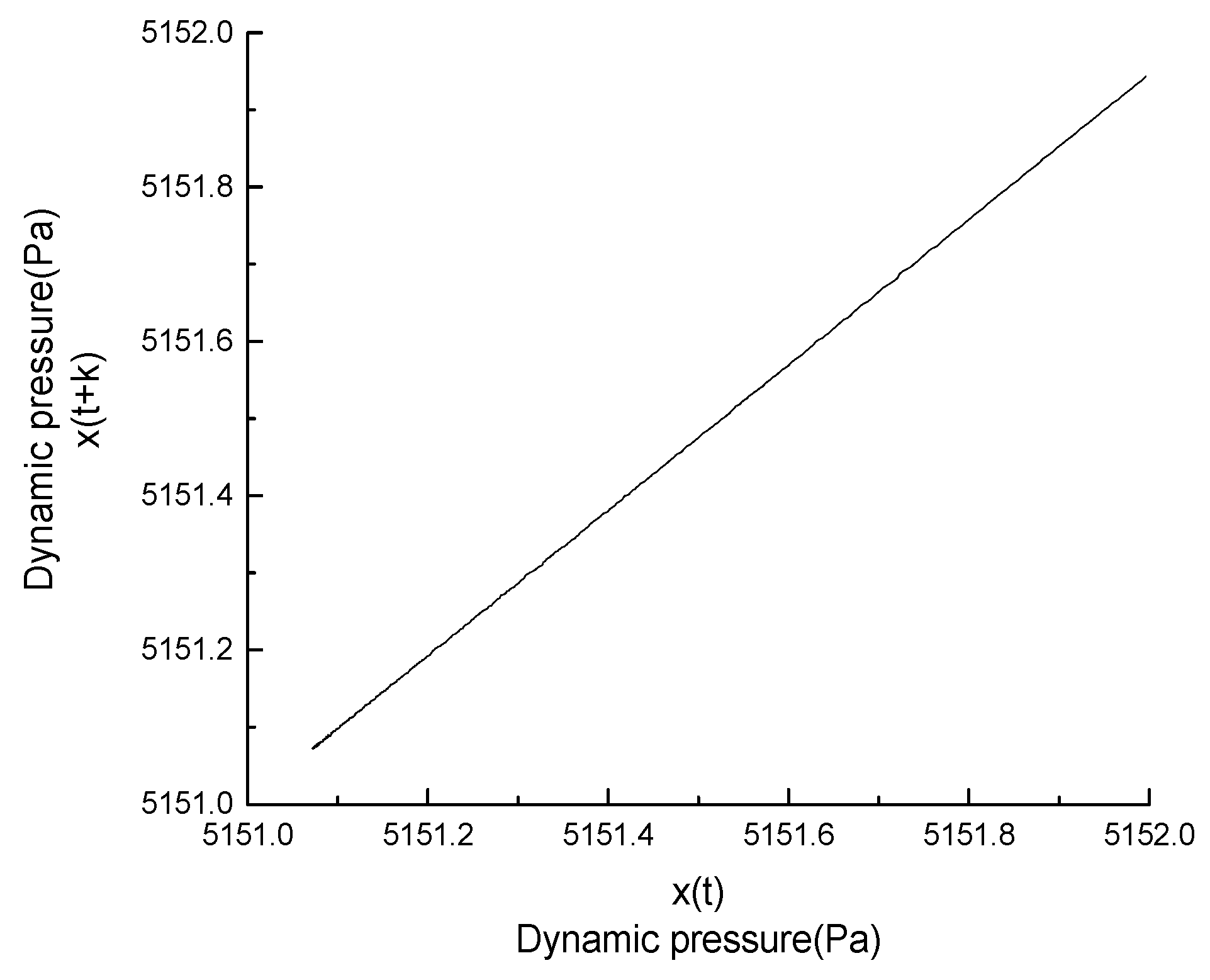
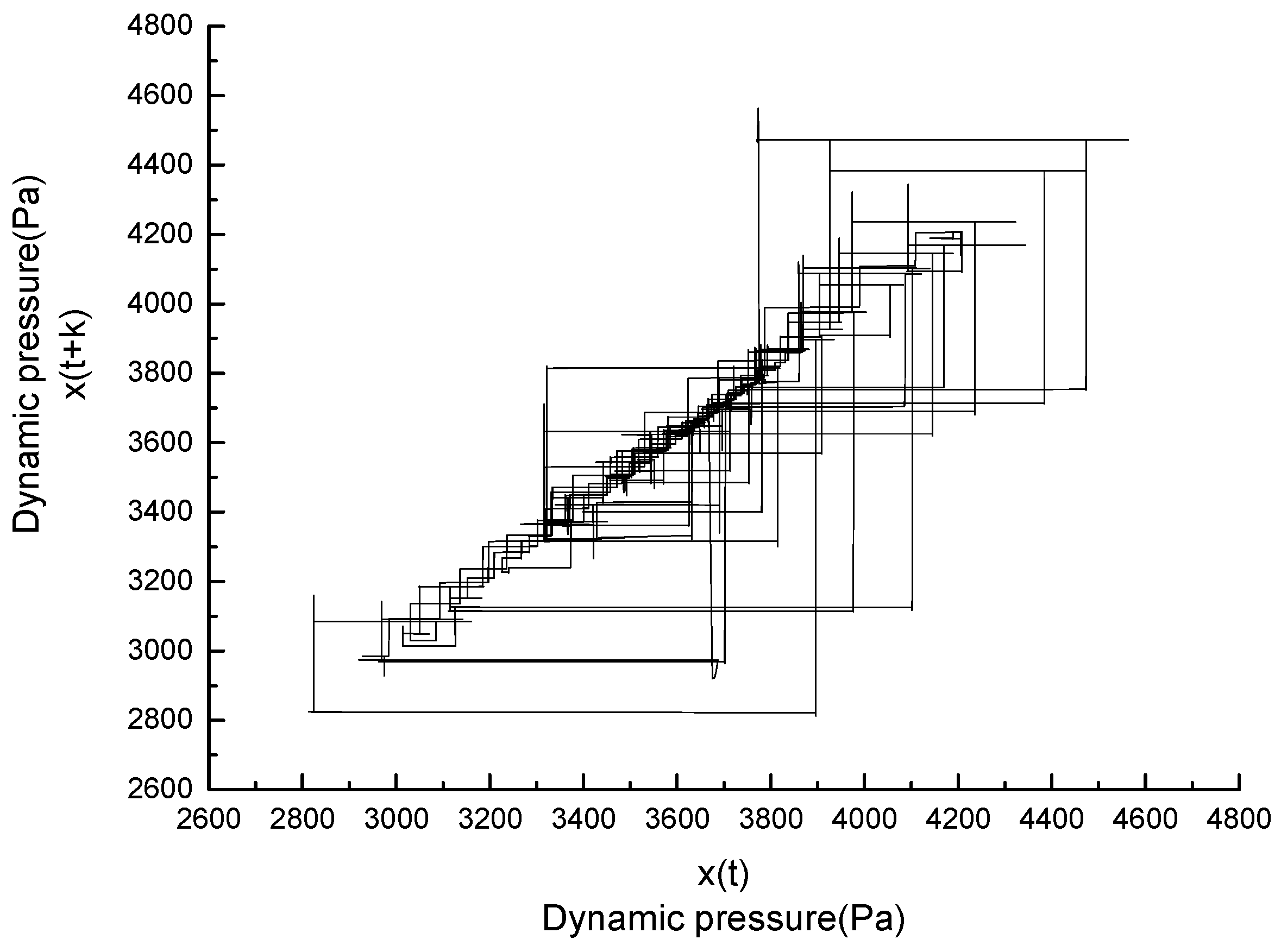
3.4. Phase Space Reconstruction in Pre- and Post- Rotating stalls

Pressure time series are obtained by the sampling points near the outlet of impeller. Figure 4 and Figure 5 are the pressure time series at P1, which are sampled both in stable and the rotating stall conditions for the centrifugal impeller.
Figure 4. Pressure time series at P1 under the stable state.
Entropy 17 07848 g004
Figure 5. Pressure time series at P1 under the rotating stall.
Entropy 17 07848 g005
From Figure 4 and Figure 5, it is found that the pressure at the impeller outlet is stable as the compressor is working well; however, the pressure at the impeller outlet shows fluctuation as the compressor enters the rotating stall condition, and the continuity of flow within the impeller becomes failed or unsatisfied.
For the accuracy, 3000 pieces of data, which are in a steady state, are selected to calculate the parameters for phase space reconstruction by the C–C method. Choosing N = 3000, m = 2 , r i = i σ / 2 , where i = 1 , 2 , 3 , 4 . Finally, the relationship between the correlation coefficient and time delay is obtained and shown in Figure 6.
The optimal time delay is the first value of S ( t ) or the first local minimum value of Δ S ( t ) , as mentioned above. As Figure 6 shows, the optimal time delay is τ = 9 . Time window is selected by the minimum values of the global τ w = 11 , and the embedding dimension can be obtained as m = 2.22 , because of τ w = ( m 1 ) τ .
Figure 6. The relationship of correlation coefficients and time delay applying the C–C method to time series at P1.
Entropy 17 07848 g006

3.4.1. Dynamics Analysis of the Pre- and Post- Rotating stall by Phase Space Reconstruction

Phase space reconstruction of the pressure time series is given with the time delay and embedding dimension which are presented above. As stated above, 3000 data from steady state are selected to reconstruct the phase space of pressure time series. Figure 7 and Figure 8 are the reconstructed phase spaces for the pressure time series at P1 under the steady and the rotating stall conditions for centrifugal impeller, respectively, so the range of pressure in Figure 7 and Figure 8 are different.
Figure 7. Phase space reconstruction for the pressure time series at P1 under the stable state.
Entropy 17 07848 g007
Figure 8. Phase space reconstruction for the pressure time series at P1 under the rotating stall. (k is the time delay.)
Entropy 17 07848 g008
Comparing Figure 7 with Figure 8, it can be seen that there is a great difference between them. It is clear that the phase portrait in the reconstructed phase space for pressure time series in a stable state is close to a straight line. However, as the compressor impeller enters the rotating stall or the flow in the impeller is in the situation of stall, the phase portrait in the reconstructed phase space for pressure time series is no longer approximate to a straight line, and it is an irregular structure which cannot be described by the traditional geometry. In Figure 8, there exist some quasi-self-similar characteristics in the graphic, and such quasi-self-similar characteristics are not fully isotropic or homogeneous, and the similarities in each direction are not exactly the same. Indeed, the geometries or sets that have the self-similarity are called fractal structures in nonlinear dynamics.
The behaviors of the system are studied by the changing of a variable. Thus, the fractal structure in the reconstructed phase space shows that the pressure time series in the rotating stall have chaotic characteristics. In other words, the fractal structure is one of the dynamics characteristics of the rotating stall.

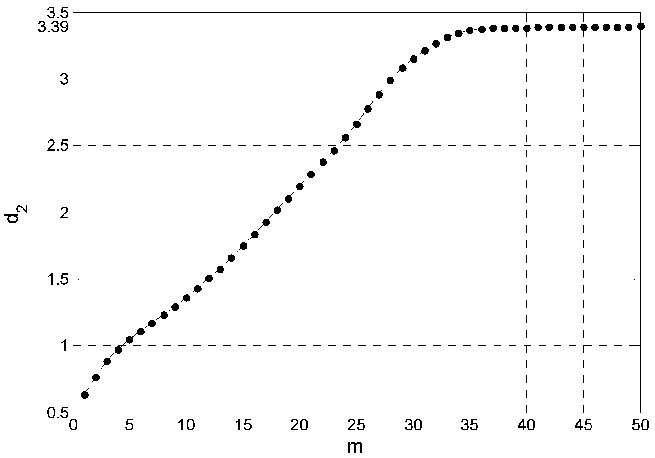
3.4.2. The Fractal Dimension in the Reconstructed Phase Space in the Post-Rotating Stall

The fractal dimension is an important characteristic of fractal dynamics, and a fractal dimension is a ratio providing a statistical index of complexity comparing how detail in a fractal pattern changes with the scale at which it is measured. Several types of fractal dimension can be measured theoretically and empirically [23]. Specifically, the correlation dimension can describe such structure more clearly than the capacity dimension and the similarity dimension.
For the system studied, the correlation dimension can be defined as,
d 2 ( m , t ) = lim r 0 ln C ( m , r , t ) ln r
where C ( m , r , t ) = lim N C ( m , N , r , t ) , and C ( m , N , r , t ) is given in Equation (2).
Figure 9 shows the fractal dimension of the fractal structure in Figure 8. With increasing of the embedding dimension, the correlation dimension no longer changes, implying reaching a limit. In Figure 9, the fractal dimension in the reconstructed phase space for pressure time series, which under the rotating stall, is 3.39.
Figure 9. Fractal dimension in the reconstructed phase space for pressure time series at P1 under the rotating stall.
Entropy 17 07848 g009

4. Phase Space Reconstruction of the Pressure Time Series at Different Locations

4.1. Parameters for Phase Space Reconstruction at Different Locations

Pressure time series at points P2, P3, P4, and P5 are collected by sampling points, and 3000 data of each are selected to be analyzed in phase space reconstruction. Using the C–C method, the parameters for phase space reconstruction can be calculated, and then the optimal time delay τ and the time window τ w , and the embedding dimension m can be obtained following τ w = ( m 1 ) τ . Finally, the parameters are given and listed in Table 1.
Table 1. Parameters for phase space reconstruction at P2, P3, P4 and P5.
P2P3P4P5
τ 12121110
τ w 15121410
m 2.252.002.272.00

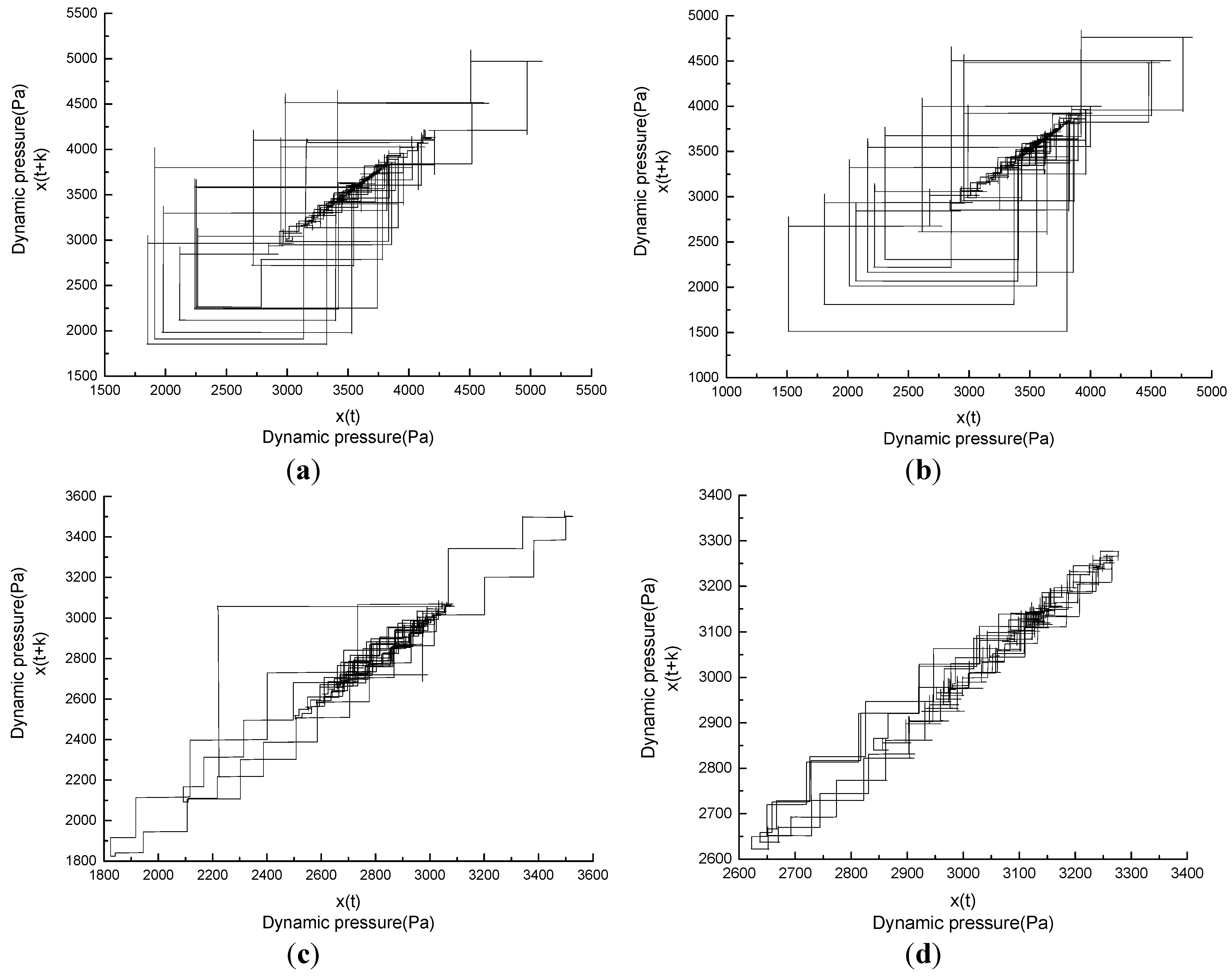
4.2. Phase Space Reconstruction for Pressure Time Series at Different Locations

Figure 10a–d shows the reconstructed phase spaces for pressure time series at P2, P3, P4 and P5 under the rotating stall state, respectively.
Figure 10. (a) Reconstructed phase space for pressure time series at P2 under the rotating stall; (b) Reconstructed phase space for pressure time series at P3 under the rotating stall; (c) Reconstructed phase space for the pressure time series at P4 under the rotating stall; (d) Reconstructed phase space for the pressure time series at P5 under the rotating stall.
Entropy 17 07848 g010
From Figure 8 and Figure 10, some quasi-self-similar geometrics are found in the reconstructed phase spaces under the rotating stall. It is shown that there are some dynamics characteristics hidden in the system, and such dynamics characteristics are important and useful to accurately identify the occurrence of the rotating stall in advance.

4.3. Fractal Dimension in the Reconstructed Phase Space for Pressure Time Series at Different Locations

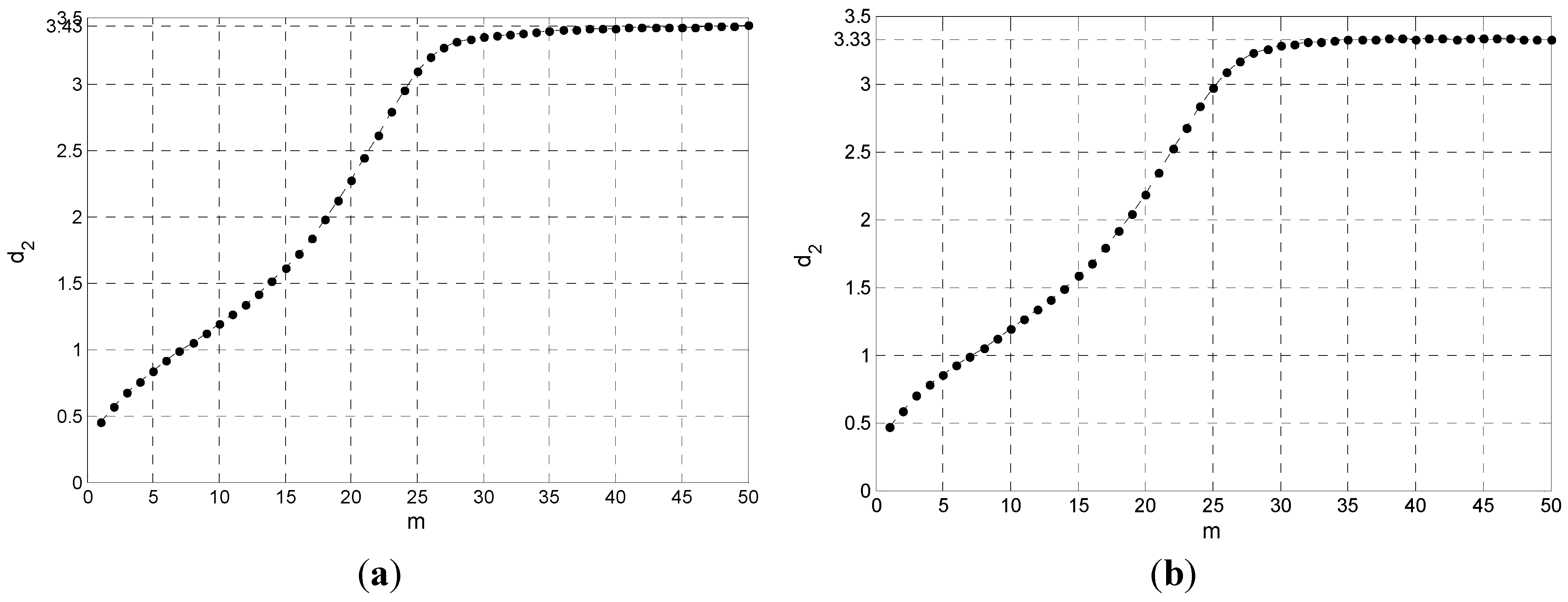
4.3.1. Fractal Dimension in the Reconstructed Phase Space at Circumference Locations

As Figure 11a,b shown, the fractal dimensions in reconstructed phase space for pressure time series at P2 and P3 under the rotating stall are 3.43 and 3.33, respectively. Compared to the fractal dimension at P1, which is 3.39, it can be drawn that the fractal dimensions in the reconstructed phase space for the pressure time series are similar in magnitude at the same radius near the impeller outlet, because the flow state is similar near the impeller outlet.
Figure 11. (a) Fractal dimension in reconstructed phase space for pressure time series at P2 under the rotating stall; (b) Fractal dimension in reconstructed phase space for pressure time series at P3 under the rotating stall.
Entropy 17 07848 g011

4.3.2. Fractal Dimensions in Reconstructed Phase Space at Different Radial Locations

As Figure 12a,b shown, the fractal dimensions in reconstructed phase spaces for pressure time series at P4 and P5 under the rotating stall are 2.66 and 2.51, respectively—in comparison with the fractal dimension at P1, which is 3.39.
Figure 12. (a) Fractal dimension in reconstructed phase space for pressure time series at P4 under the rotating stall; (b) Fractal dimension in reconstructed phase space for pressure time series at P5 under the rotating stall.
Entropy 17 07848 g012
Furthermore, a comparison with the fractal dimensions at different locations in reconstructed phase space is given and some results can be obtained. As the sampling points are at the same radius, the flow state and the pressure fluctuation are similar, and so the fractal dimension changes slightly. As the sampling points keep away from the impeller outlet, both the flow state and the pressure fluctuation change, and so the fractal dimension in reconstructed phase space for pressure time series becomes less, because the complexity of flow becomes higher when the flow runs away from the impeller outlet. In a word, it is indicated that the fractal dimension can measure the complexity of flow in a post-the rotating stall near the impeller outlet.

5. Conclusions

There are some significant differences in reconstructed phase space of pressure time series between pre- and post- rotating stalls in centrifugal impeller. In the rotating stall state, there exist some quasi-self-similar structures in the reconstructed phase space, which can be considered as fractal structure. Further, the fractal structure shows that the pressure time series near the impeller outlet in the rotating stall state is not random, and such fractal structure as the dynamic characteristics of the rotating stall is beneficial to identify the rotating stall and control it.
In addition, the correlation dimension is one of the fractal dimensions, which is an important characteristic of fractal structure. The results show that the correlation dimension can be used to describe the fractal structure, and the fractal dimension can capture the dynamic characteristics of the rotating stall more accurately.
Furthermore, the fractal dimensions in different locations show that the fractal dimensions are close at the same radius near the impeller outlet, and as the location is away from the impeller outlet, the fractal dimension decreases. These quantitative changes are available to use to measure complexity of flow in post-the rotating stalls at different locations near the impeller outlet.

Acknowledgments

The authors would like to thank the reviewers for their valuable comments and suggestions to improve the present work. This article is contributed by the National Basic Research Program of China (973 Program, Grant No. 2012CB026002), the National Key Technology Research and Development Program of the Ministry of Science and Technology of China (Grant No. 2013BAF01B02) and the National Natural Science Foundation of China, (Grant No. 51305355).

Author Contributions

Jiazhong Zhang designed the research. Le Wang and Wenfan Zhang performed the numerical simulation and analyzed the data. All authors have read and approved the final version of the manuscript.

Conflicts of Interest

The authors declare no conflict of interest.

References

  1. Stein, A.; Niazi, S.; Sankar, L.N. Computational Analysis of Stall and Separation Control in Centrifugal Compressors. J. Propuls. Power 2000, 16, 65–71. [Google Scholar] [CrossRef]
  2. Stein, A.; Niazi, S.; Sankar, L.N. Computational Analysis of Centrifugal Compressor Surge Control Using Air Injection. J. Aircr. 2001, 38, 513–520. [Google Scholar] [CrossRef]
  3. Taher, H.; Mohamed, A.; Osama, B.; Mohamed, S.G. Numerical Investigation of The rotating stall Characteristics and Active Stall Control in Centrifugal Compressors. In Proceedings of the ASME 2014 Power Conference, Baltimore, MD, USA, 28–31 July 2014.
  4. Day, I.J.; Greitzer, E.M.; Cumpsty, N.A. Prediction of Compressor Performance in The rotating stall. J. Eng. Power 1978, 100, 1–14. [Google Scholar] [CrossRef]
  5. Day, I.J. Stall Inceptionin Axial Flow Compressor. J. Turbomach. 1993, 115, 1–9. [Google Scholar] [CrossRef]
  6. Tan, C.S.; Day, I.J.; Morris, S.; Wadia, A. Spike-Type Compressor Stall Inception Detection and Control. Annu. Rev. Fluid Mech. 2010, 42, 275–300. [Google Scholar] [CrossRef]
  7. Greitzer, E.M. Review—Axial Compressor Stall Phenomenon. J. Fluids Eng. 1980, 102, 134–151. [Google Scholar] [CrossRef]
  8. Fink, D.A.; Cumpsty, N.A.; Greitzer, E.M. Surge Dynamics in a Free-Spool Centrifugal Compressor System. J. Turbomach. 1992, 114, 321–332. [Google Scholar] [CrossRef]
  9. Chima, R.V.; Yokota, J.W. Numerical Analysis of Three-Dimensional Viscous Internal Flows. AIAA J. 1990, 28, 798–806. [Google Scholar] [CrossRef]
  10. Xu, C.; Amano, R.S. Study of the Flow in Centrifugal Compressor. In Proceedings of the ASME Turbo Expo 2009: Power for Land, Sea, and Air, Orlando, FL, USA, 8–12 June 2009.
  11. Liu, Y.; Li, K.; Zhang, J.; Wang, H.; Liu, L. Numerical Bifurcation Analysis of Static Stall of Airfoil and Dynamic Stall under Unsteady Perturbation. Commun. Nonlinear Sci. Numer. Simul. 2012, 17, 3427–3434. [Google Scholar] [CrossRef]
  12. Seely, A.J.E.; Newman, K.D.; Herry, C.L. Fractal Structure and Entropy Production within the Central Nervous System. Entropy 2014, 16, 4497–4520. [Google Scholar] [CrossRef]
  13. Packard, N.H.; Crutchfield, J.P.; Farmer, J.D.; Shaw, R.S. Geometry from a time Series. Phys. Rev. Lett. 1980, 45, 712–716. [Google Scholar] [CrossRef]
  14. Joseph, D.D.; Chen, T.S. Friction Factors in theory of Bifurcating Poiseuille Flow through Annular Ducts. J. Fluid Mech. 1974, 66, 189–207. [Google Scholar] [CrossRef]
  15. Farmer, M.E. Chaotic Phenomena from Motion in Image Sequences. In Proceedings of the International Joint Conference on Neural Networks 2007 (IJCNN 2007), Orlando, FL, USA, 12–17 August 2007.
  16. Bright, M.M. Chaotic Time Series Analysis Tool for Identification and Stabilization of the Rotating Stall Precursor Events in High Speed Compressor. Ph. D. Thesis, Akron University, Akron, OH, USA, 2000. [Google Scholar]
  17. Gu, Y.; Zhou, Z.; Li, Y. Characteristic of fan stalling based on correlated dimensions. Trans. Nanjing Univ. Aeronaut. Astronaut. 2011, 28, 362–366. [Google Scholar]
  18. Hathaway, M.D.; Chriss, R.M.; Strazisar, A.J.; Wood, J.R. Laser Anemometer Measurement of the Three-Dimensional Rotor Flow Field in the NASA Low-Speed Centrifugal Compressor. Available online: http://ntrs.nasa.gov/archive/nasa/casi.ntrs.nasa.gov/19950025564.pdf (accessed on 17 November 2015).
  19. Takens, F. Detecting Strange Attractors in Turbulence. In Dynamical Systems and Turbulence, Warwick 1980; Springer: Berlin, Germany, 1981; Volume 898, pp. 366–381. [Google Scholar]
  20. Grassgerber, P.; Prociccia, I. Measuring the strangeness of strange attractors. Phys. D 1983, 9, 189–208. [Google Scholar] [CrossRef]
  21. Kugiumtzis, D. State space reconstruction parameters in the analysis of chaotiic time series-the role of the time widow length. Phys. D 1996, 95, 13–28. [Google Scholar] [CrossRef]
  22. Kim, H.S.; Eykholt, R.; Salas, J.D. Nonlinear dynamics, delay time and embedding windows. Phys. D 1999, 127, 48–60. [Google Scholar] [CrossRef]
  23. Falconer, K. Fractal Geometry: Mathematical Foundations and Applications; Wiley: New York, NY, USA, 2004. [Google Scholar]

