
An Information-Based Approach to Precision Analysis of Indoor WLAN Localization Using Location Fingerprint

Abstract
:1. Introduction
2. Related Work
3. System Description
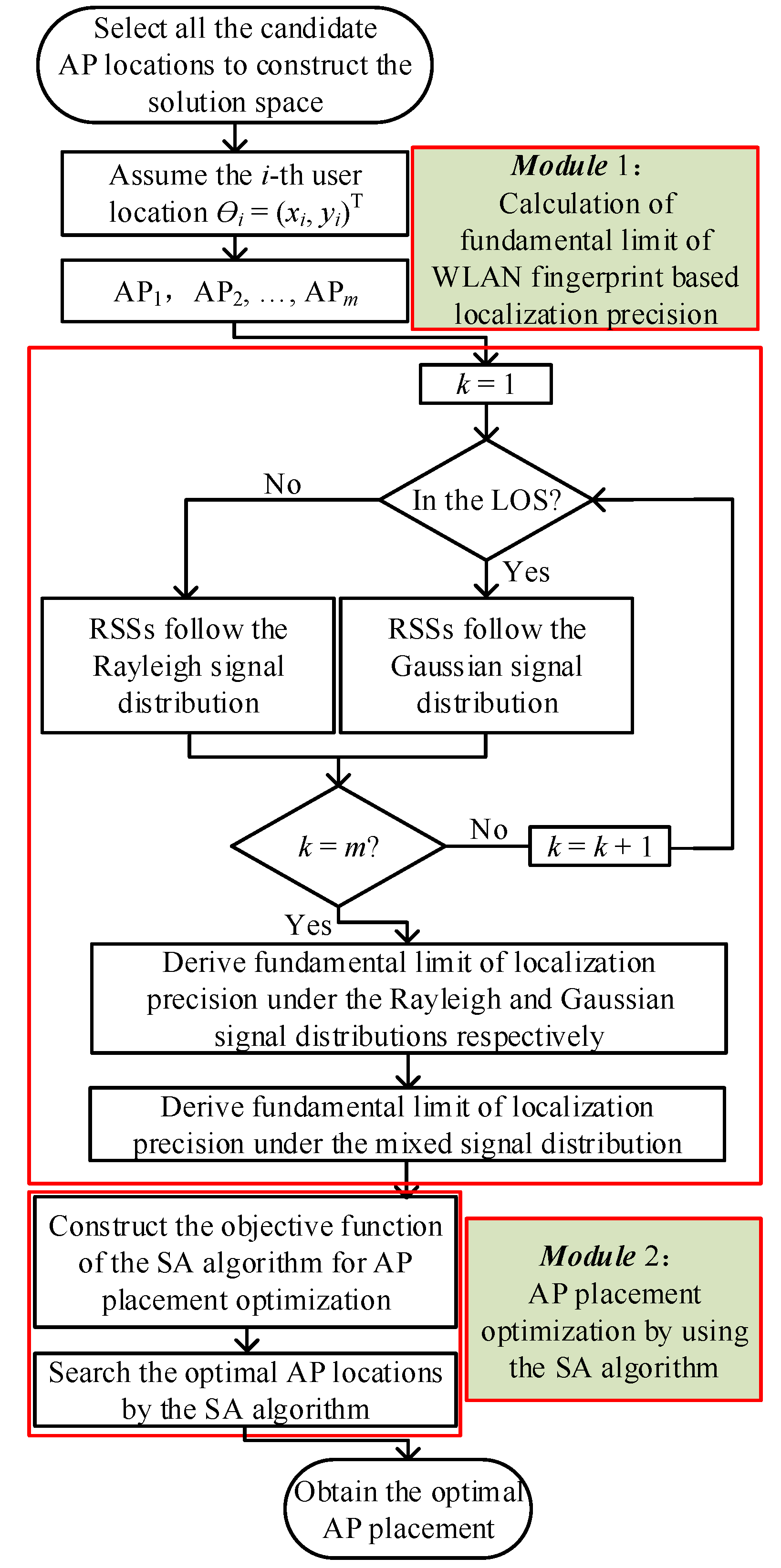
3.1. System Overview

3.2. Fundamental Limit of Localization Precision
3.2.1. Localization Precision vs. Signal Distributions
Analysis with Gaussian signal distribution

Analysis with Rayleigh signal distribution
3.2.2. Impact of the AP Number


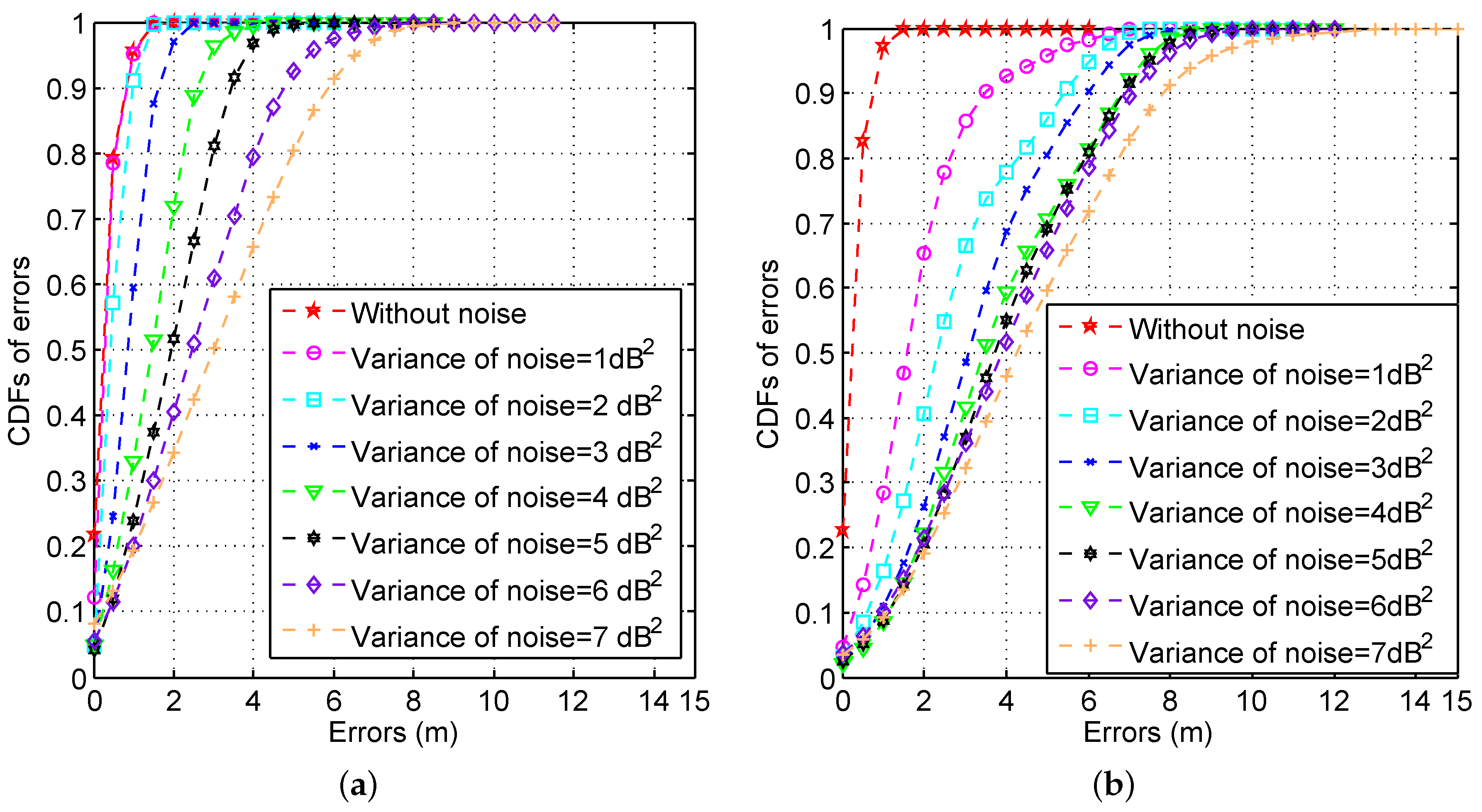
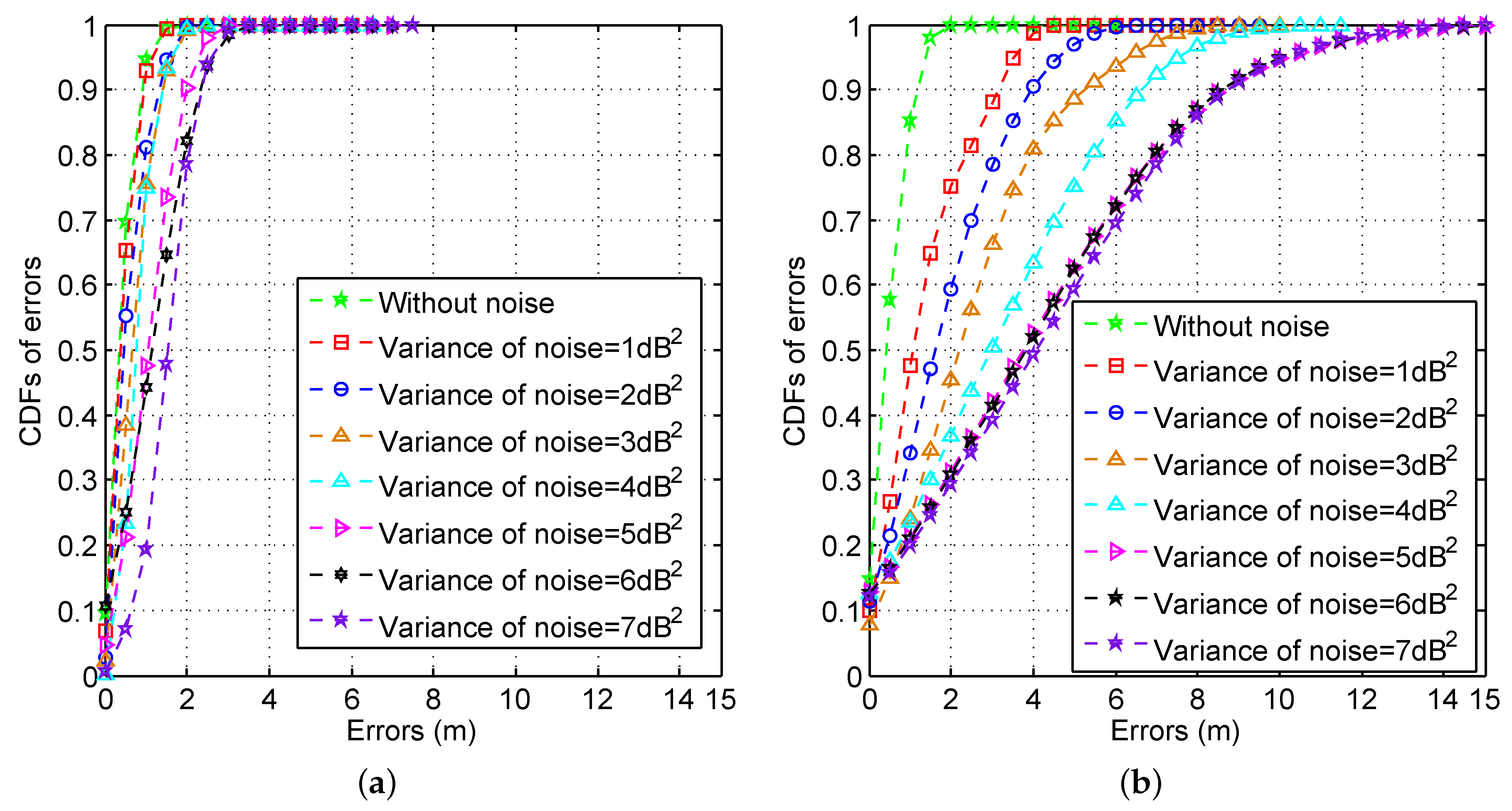
3.2.3. Impact of Noise Variance


3.2.4. Fundamental Limit with a Mixed Signal Distribution
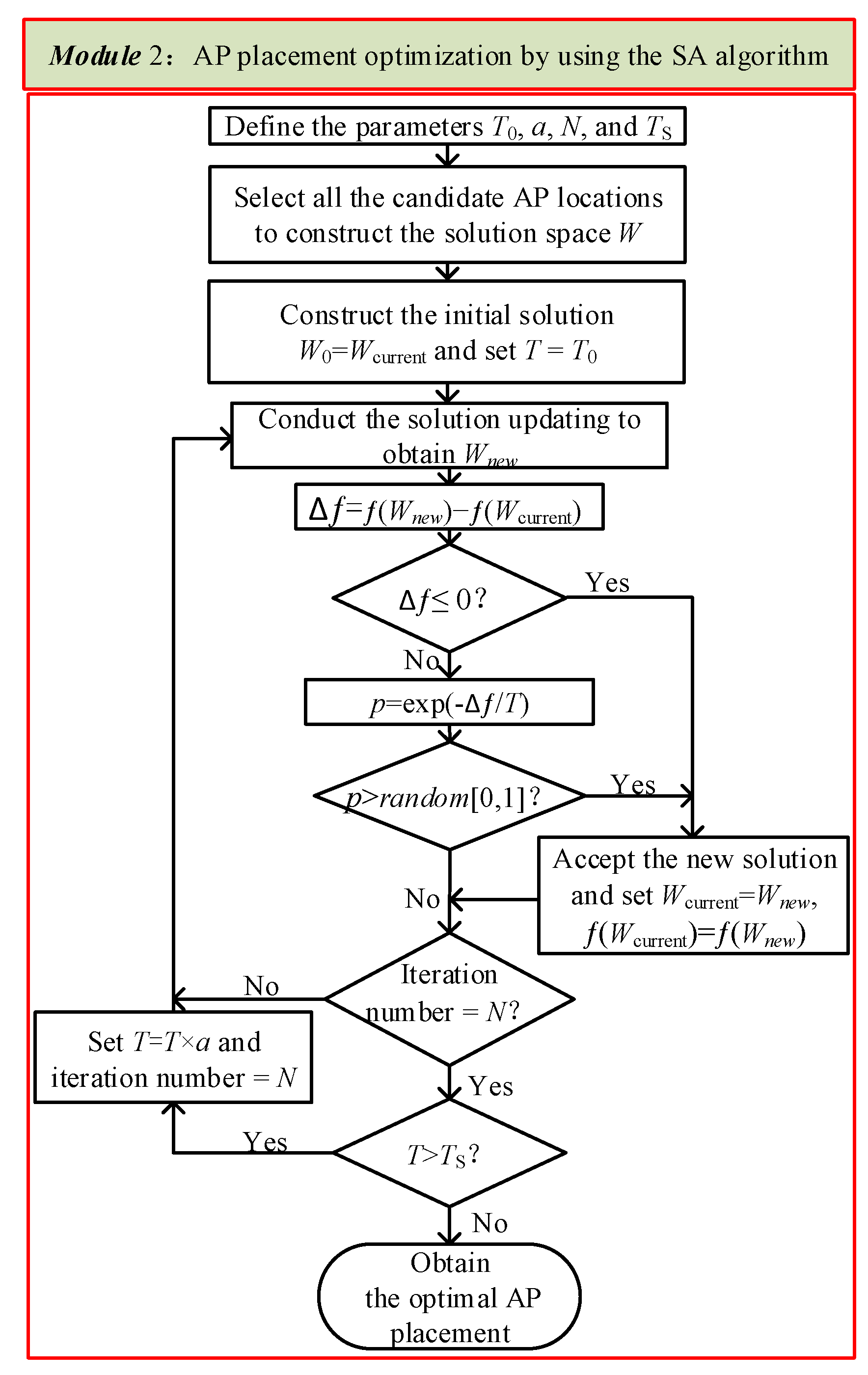
3.3. AP Placement Optimization

4. Simulation Results

| Parameters | Values |
|---|---|
| Platform | MATLAB 7.0 |
| Carrier frequency | 2.4 GHz |
| −28 dBm | |
| β | 2.2 |
| Number of candidate AP locations | 144 (LOS), 176 (NLOS) |
| Number of RPs | 144 (LOS), 176 (NLOS) |
| Number of test points | 100 |
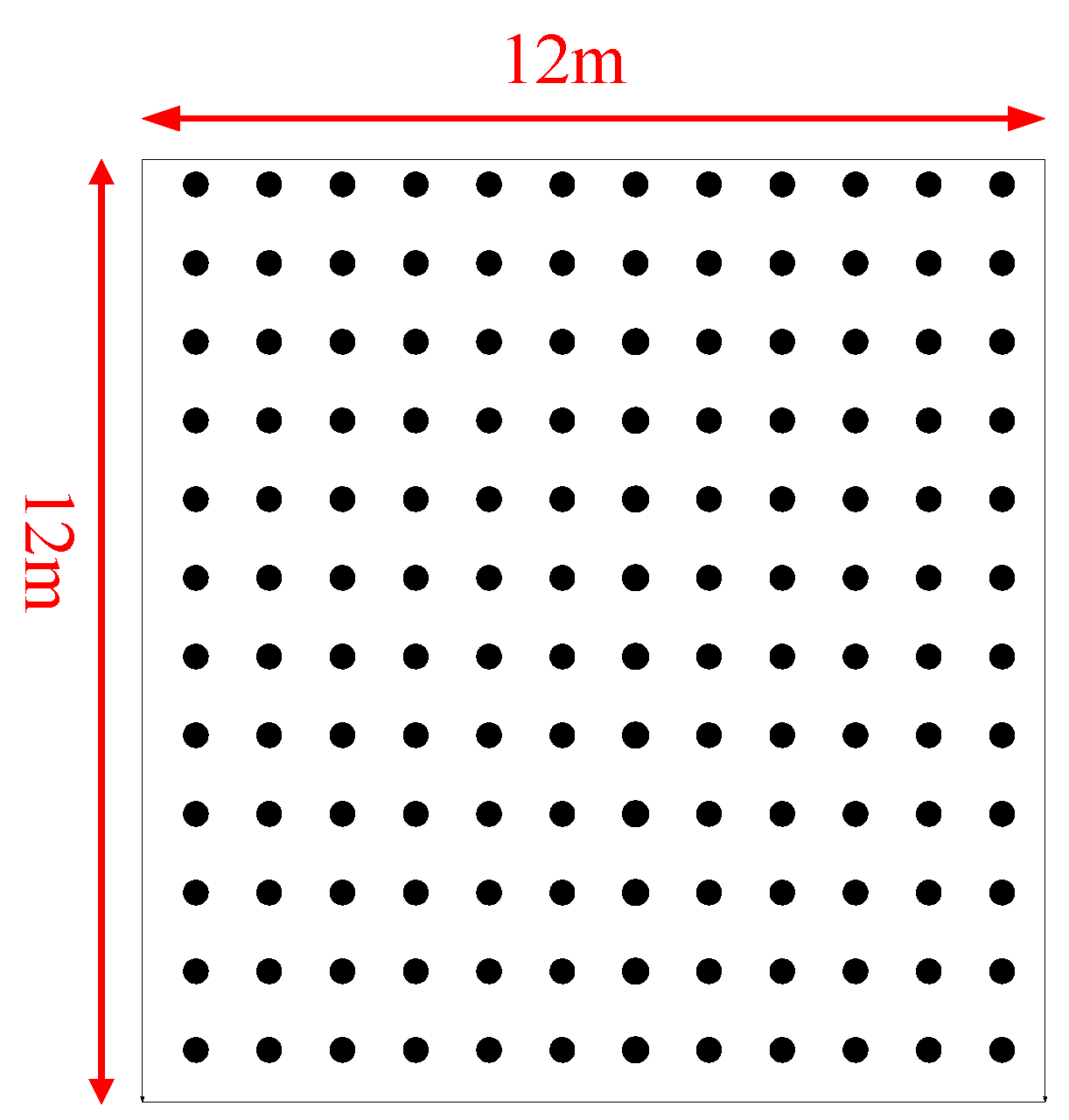
| Dimensions of the target environment | (LOS), (NLOS) |
| k | 3 |
| 200 | |
| N | 500 |
| α | 0.95 |
| 0.1 | |
| 10 |
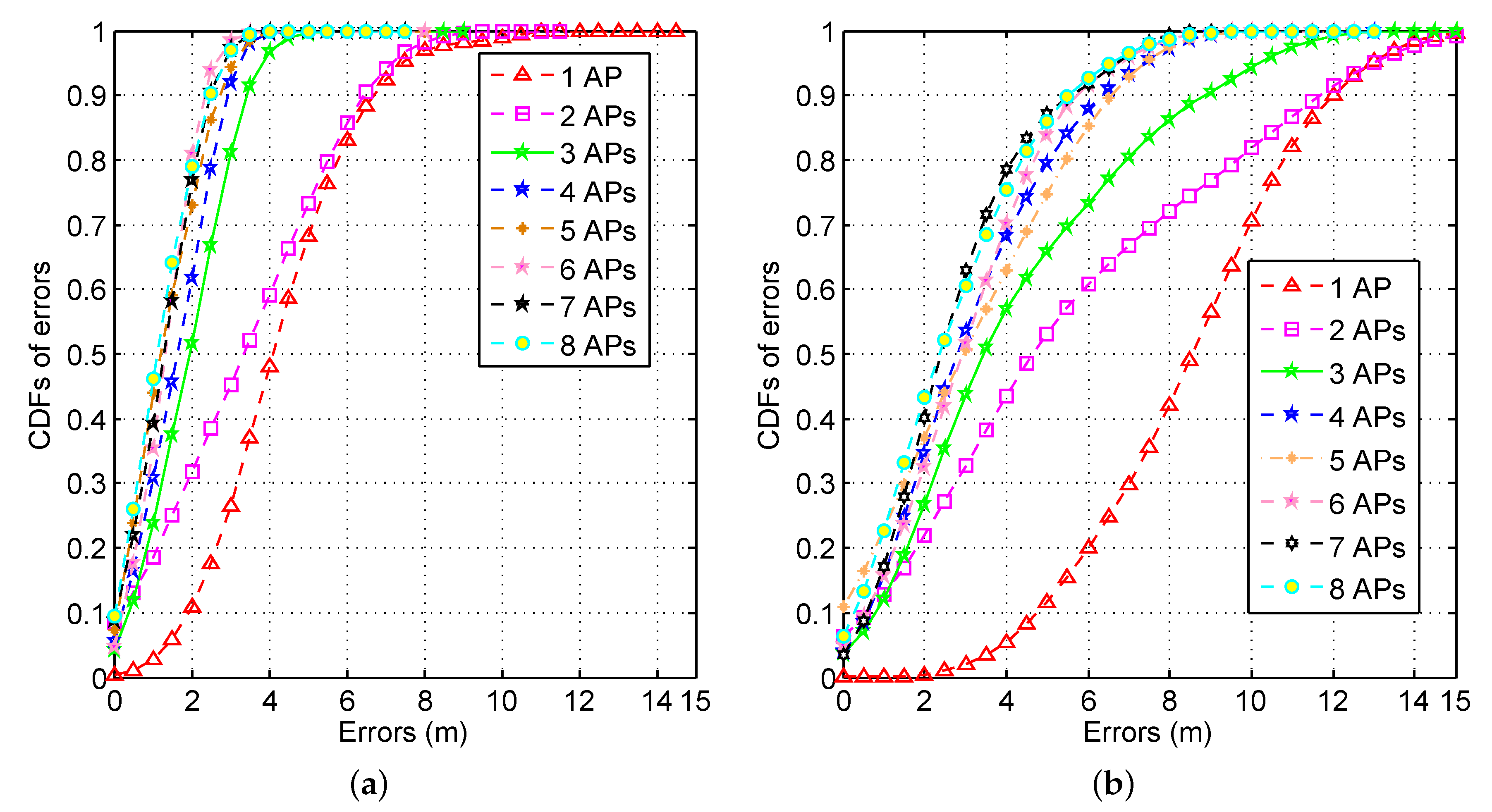
4.1. Regular LOS Environment


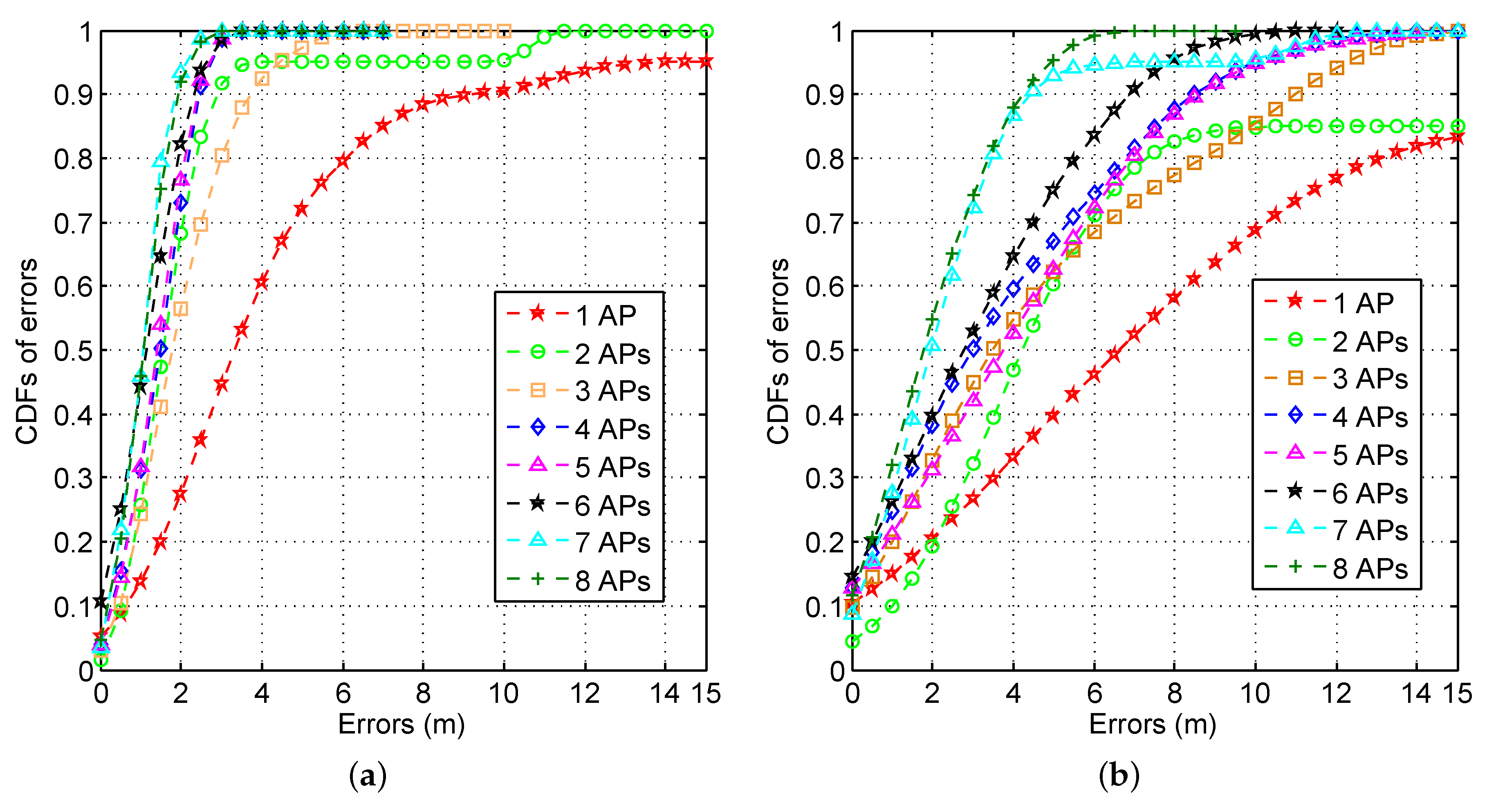
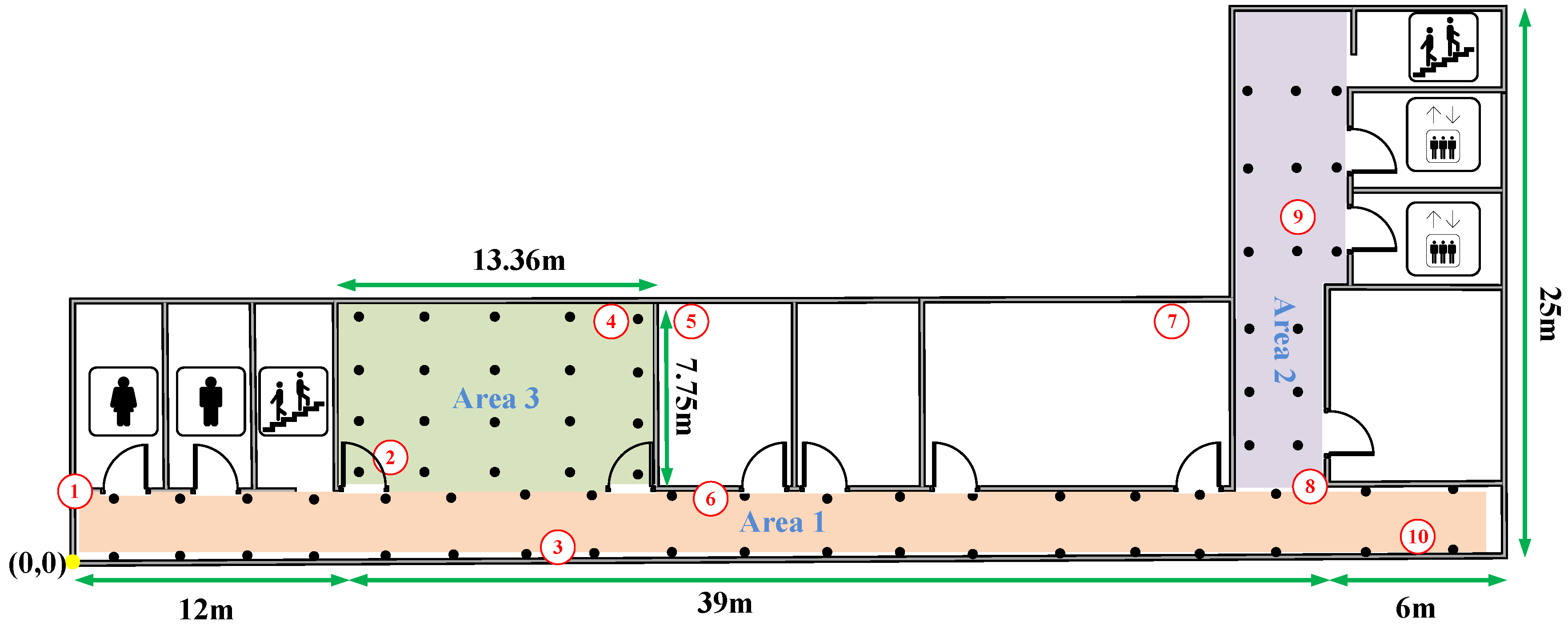
4.2. Irregular NLOS Environment


4.3. Computation Overhead


5. Discussion


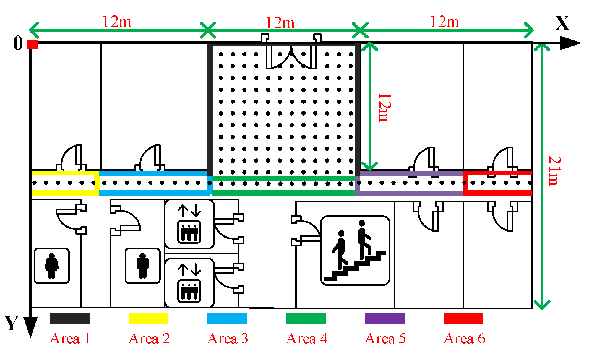
6. Case Study


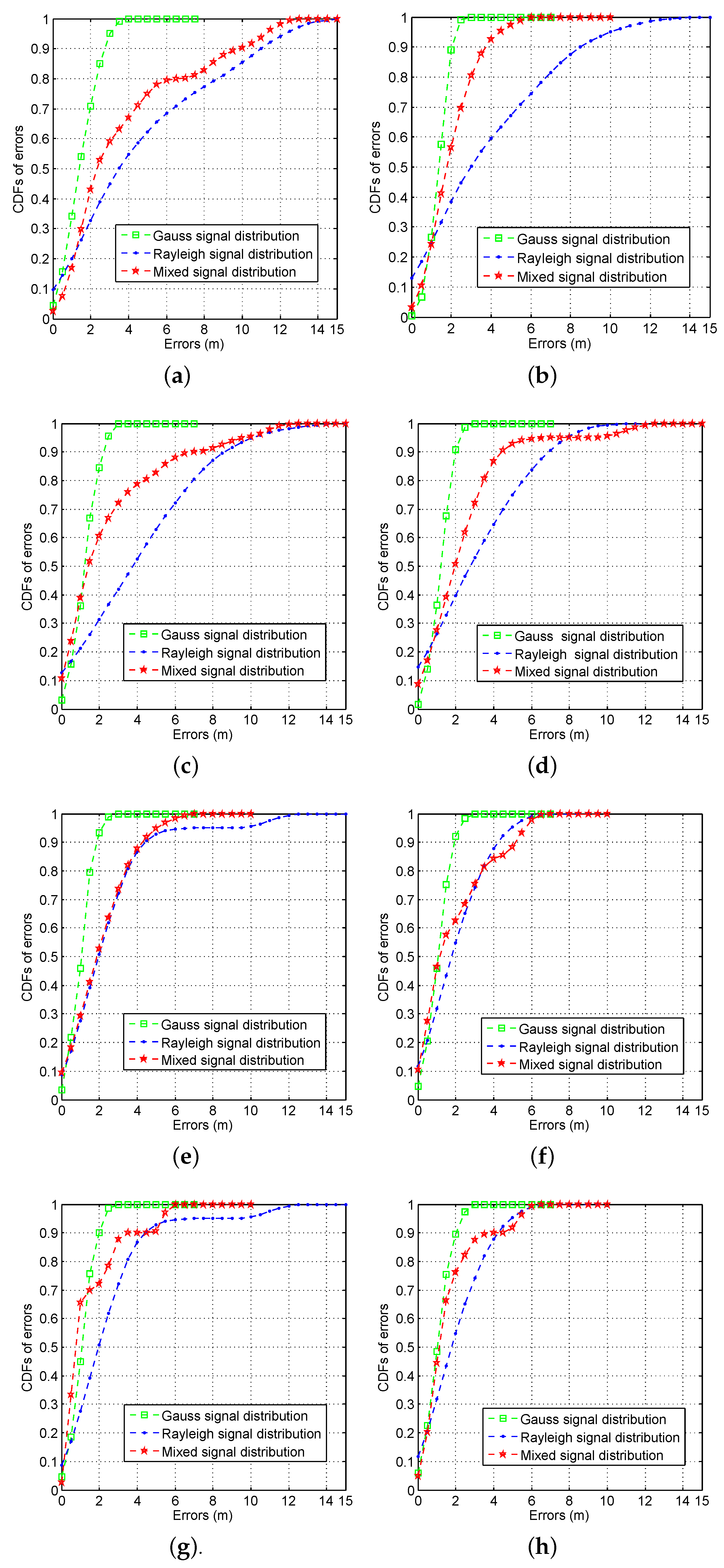
6.1. CDFs of Errors with Different AP Numbers

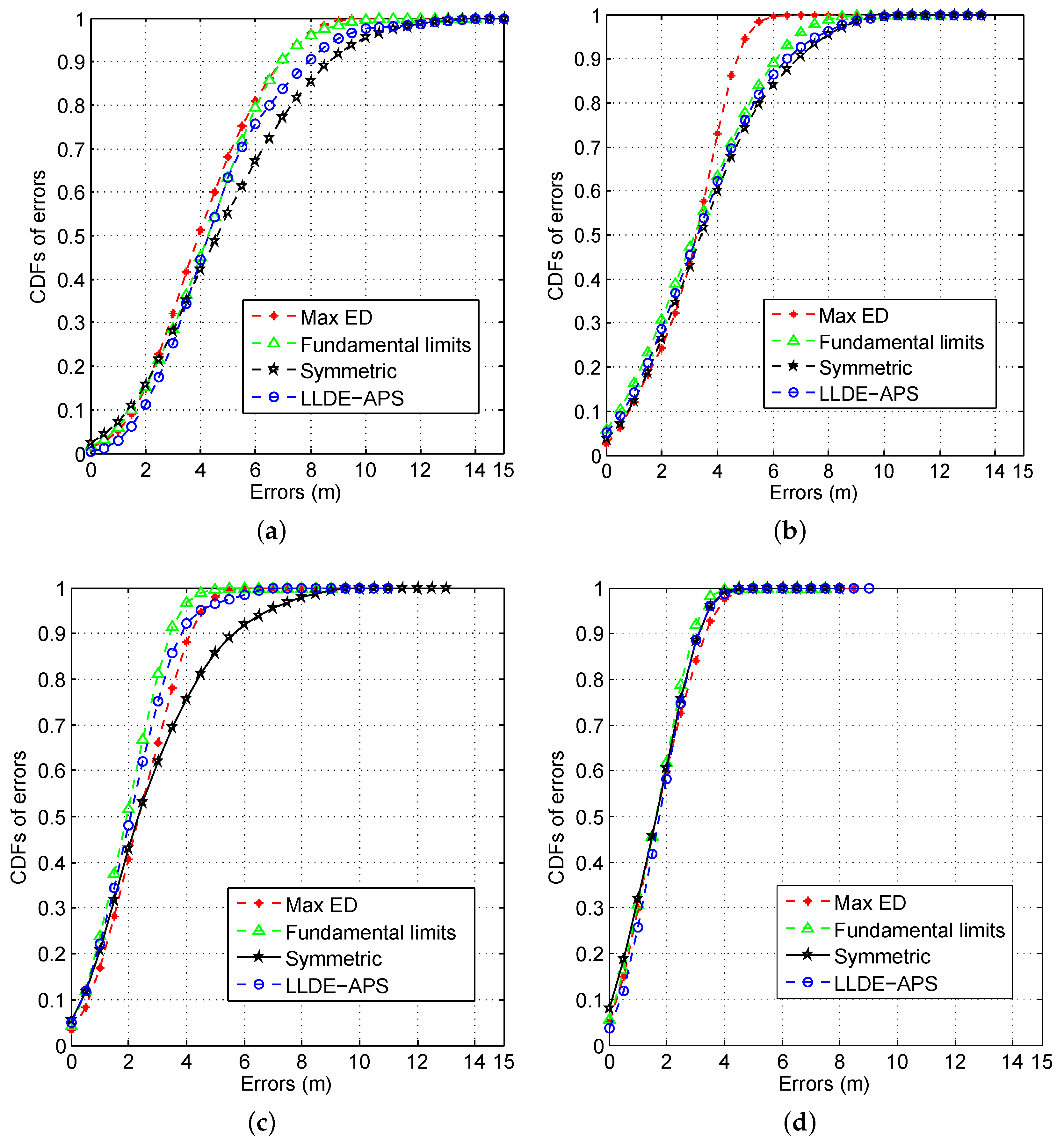
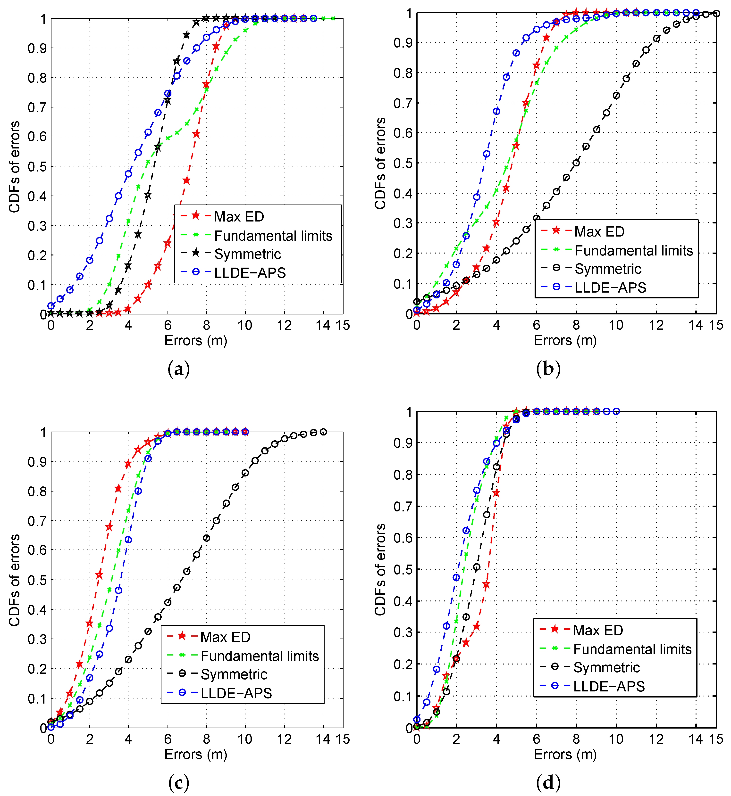
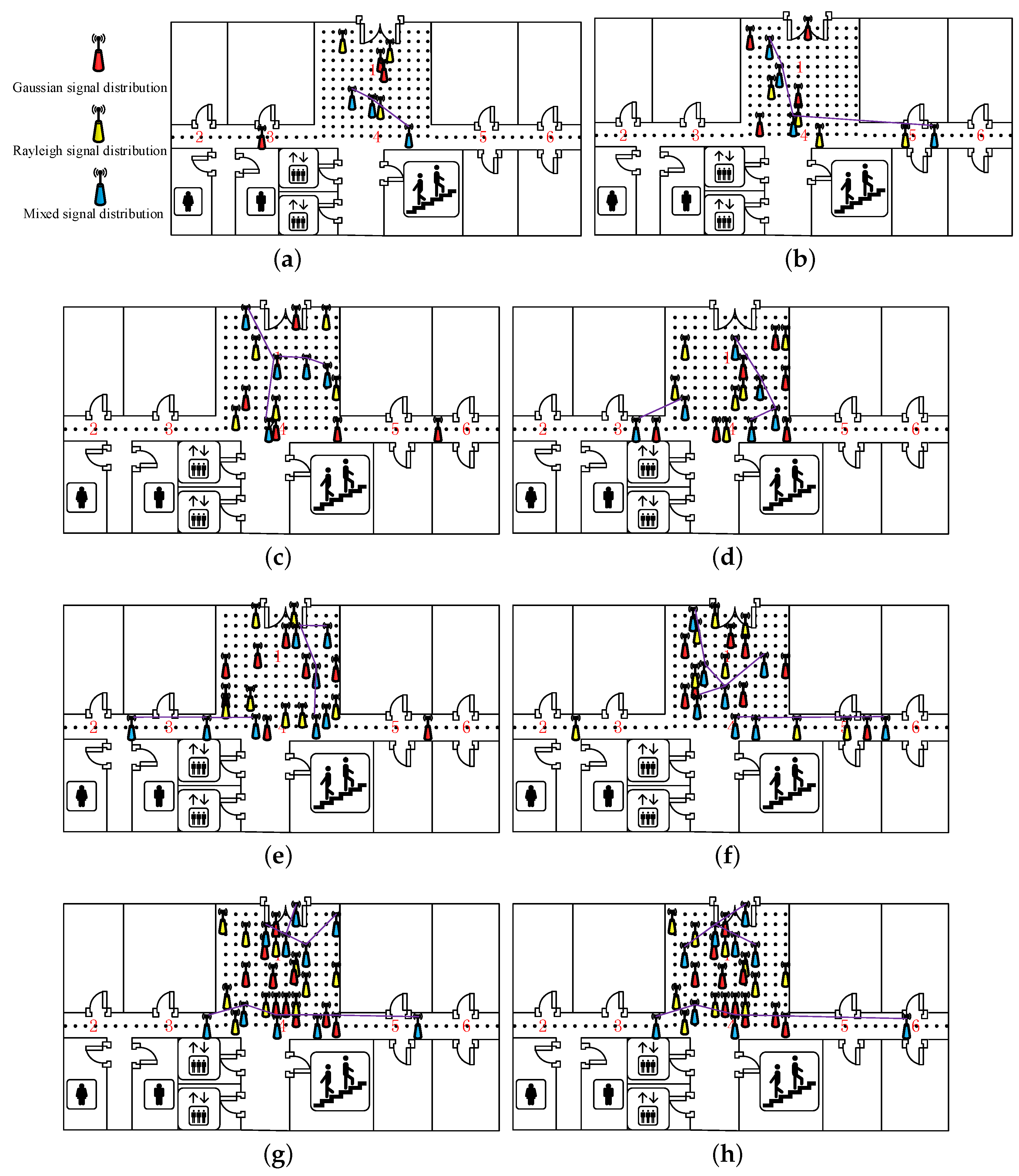
6.2. CDFs of Errors by Using Different AP Optimization Approaches

6.3. Positioning Errors under Different Signal Distributions
| AP Number | Gaussian Signal Distribution | Rayleigh Signal Distribution | Mixed Signal Distribution |
|---|---|---|---|
| 2 | 3.884 m | 5.360 m | 3.225 m |
| 3 | 2.911 m | 2.974 m | 2.701 m |
| 4 | 2.494 m | 2.210 m | 2.210 m |
| 5 | 2.255 m | 1.966 m | 1.966 m |
| 6 | 2.032 m | 1.884 m | 1.954 m |
| 7 | 1.8998 m | 1.819 m | 1.819 m |
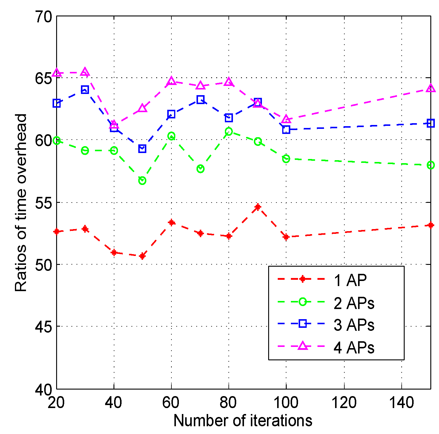
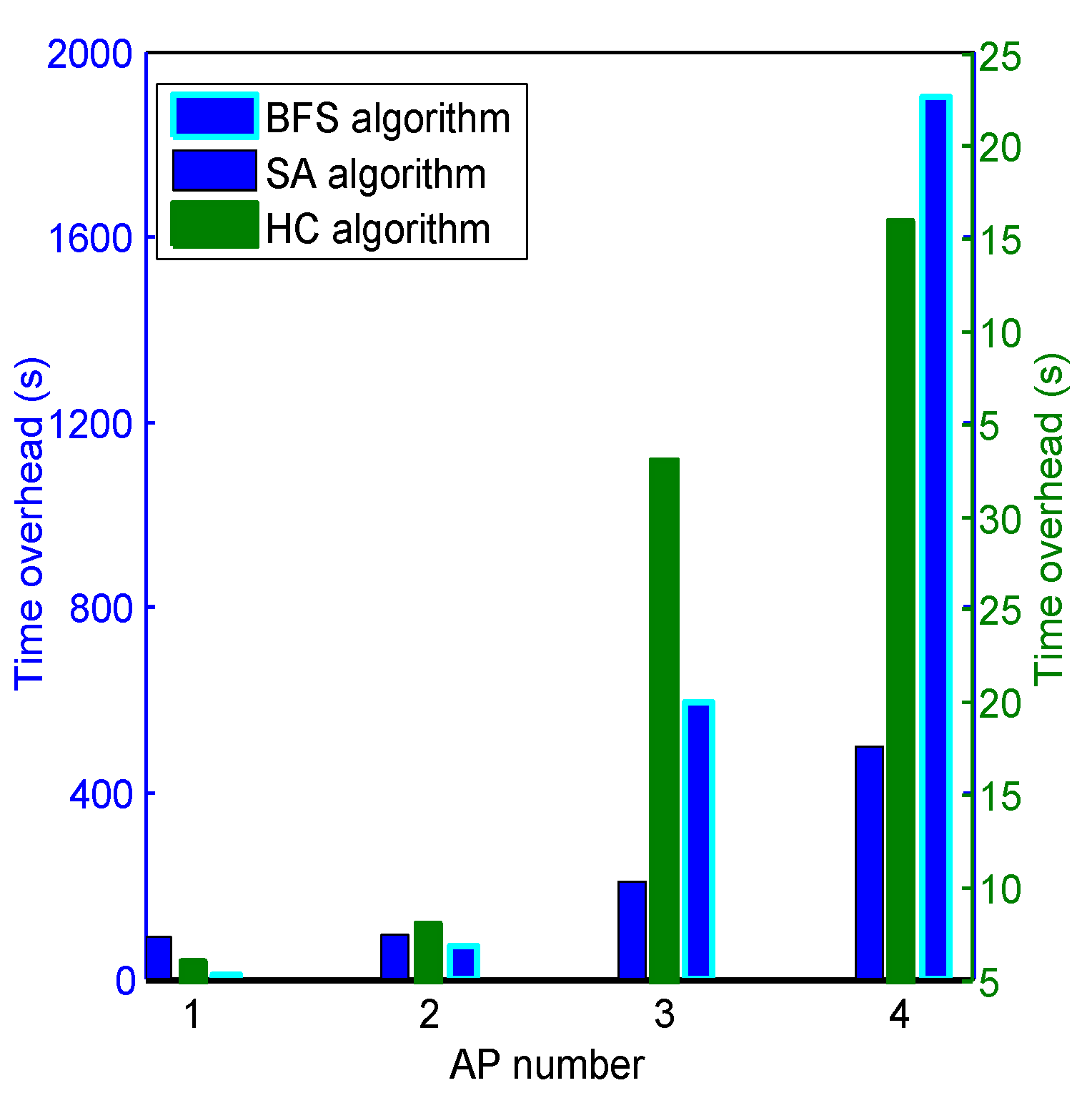
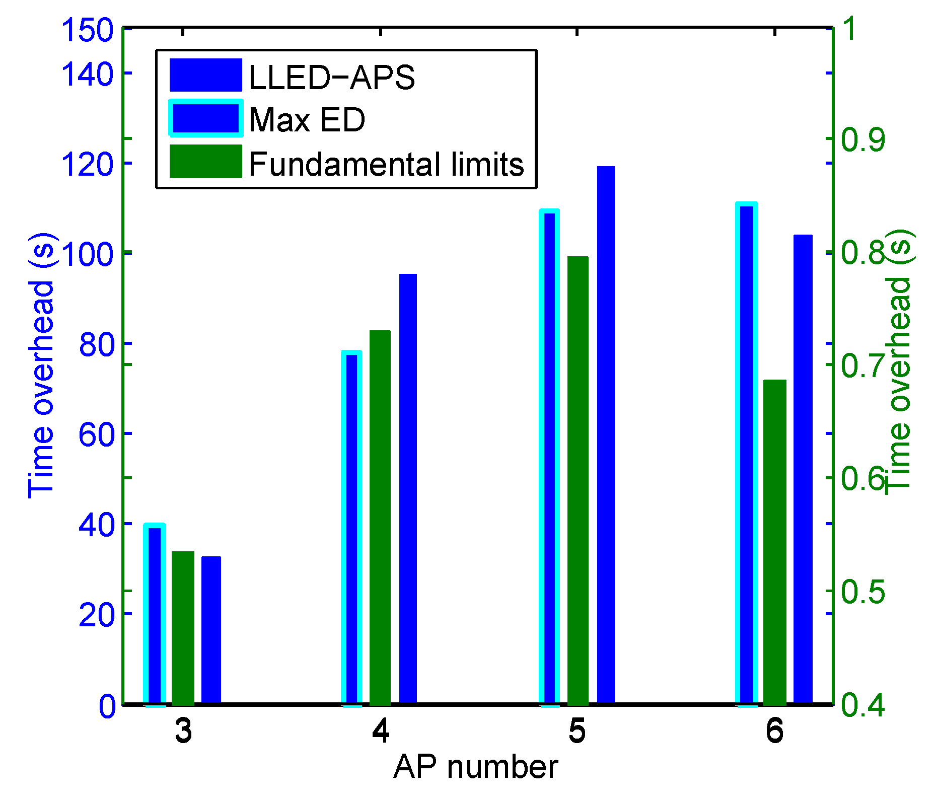
6.4. Time Overhead by Using Different AP Optimization Approaches

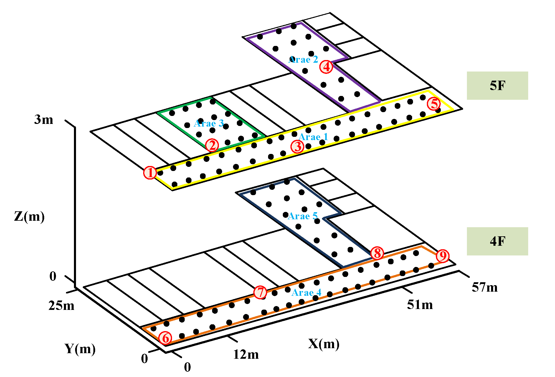
6.5. Extension to a Multi-Floor Environment

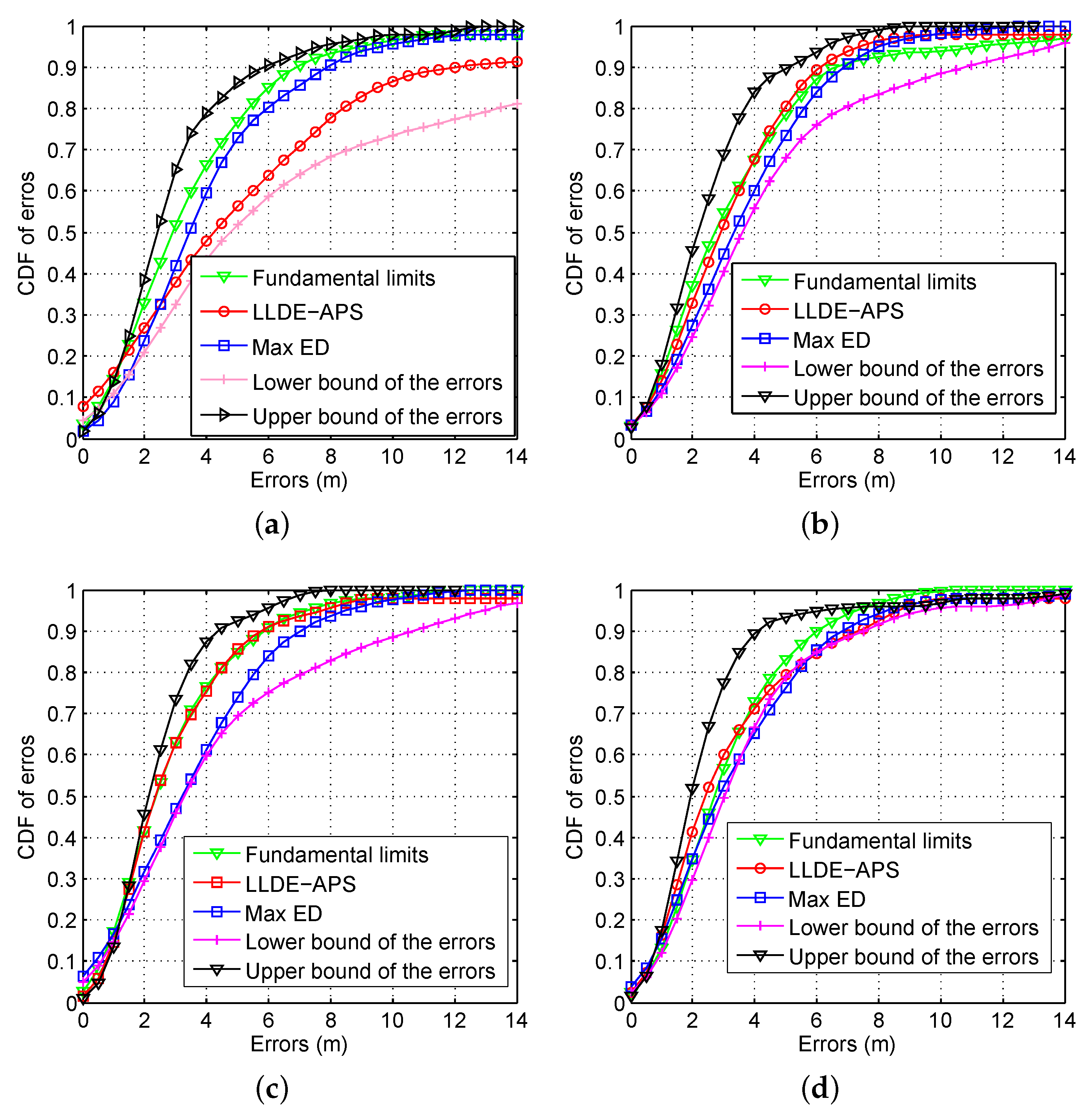
6.5.1. CDFs of Errors by Using Different AP Optimization Approaches

6.5.2. Positioning Errors under Different Signal Distributions
| AP Number | Gaussian Signal Distribution | Rayleigh Signal Distribution | Mixed Signal Distribution |
|---|---|---|---|
| 3 | 5.07 m | 3.65 m | 3.65 m |
| 4 | 3.55 m | 3.59 m | 3.26 m |
| 5 | 3.25 m | 3.31 m | 3.19 m |
| 6 | 3.12 m | 3.32 m | 3.12 m |
| 7 | 3.08 m | 2.93 m | 2.87 m |
| 8 | 2.87 m | 3.02 m | 2.78 m |
| 9 | 2.77 m | 2.77 m | 2.77 m |
| AP Number | Gaussian Signal Distribution | Rayleigh Signal Distribution | Mixed Signal Distribution |
|---|---|---|---|
| 3 | ③⑤⑨ | ④⑥⑦ | ④⑥⑦ |
| 4 | ③④⑤⑦ | ①④⑦⑧ | ④⑤⑥⑦ |
| 5 | ③④⑥⑦⑧ | ①③⑥⑧⑨ | ②④⑥⑦⑧ |
| 6 | ②③④⑥⑧⑨ | ①③⑤⑥⑦⑧ | ②③④⑥⑦⑧ |
| 7 | ②③⑤⑥⑦⑧⑨ | ③④⑤⑥⑦⑧⑨ | ①②③④⑥⑦⑧ |
| 8 | ①②③④⑤⑥⑦⑧ | ①③④⑤⑥⑦⑧⑨ | ①②③④⑥⑦⑧⑨ |
| 9 | ①②③④⑤⑥⑦⑧⑨ | ①②③④⑤⑥⑦⑧⑨ | ①②③④⑤⑥⑦⑧⑨ |
7. Conclusions
Acknowledgments
Author Contributions
Conflicts of Interest
References
- Zhou, M.; Wong, A.K.-S.; Tian, Z.; Luo, X.; Xu, K.; Shi, R. Personal mobility map construction for crowd-sourced Wi-Fi based indoor mapping. IEEE Commun. Lett. 2014, 18, 1427–1430. [Google Scholar] [CrossRef]
- Zhou, M.; Zhang, Q.; Xu, K.; Tian, Z.; Wang, Y.; He, W. PRIMAL: Page rank-based indoor mapping and localization using gene-sequenced unlabeled WLAN received signal strength. Sensors 2015, 15, 24791–24817. [Google Scholar] [CrossRef] [PubMed]
- Chen, Q.; Huang, G.; Song, S. WLAN User Location Estimation Based on Receiving Signal Strength Indicator. In Proceedings of the 5-th International Conference on Wireless Communications, Networking and Mobile Computing, Beijing, China, 24–26 September 2009.
- Guyen, G.K.; Nguyen, T.V.; Shin, H. Learning Dictionary and Compressive Sensing for WLAN Localization. In Proceedings of the IEEE Wireless Communications and Networking Conference (WCNC), Istanbul, Turkey, 6–9 April 2014; pp. 2910–2915.
- Zhou, M.; Wong, A.K.; Tian, Z.; Zhang, V.Y.; Yu, X.; Lou, X. Adaptive mobility mapping for people tracking using unlabelled Wi-Fi shotgun reads. IEEE Commun. Lett. 2013, 17, 87–90. [Google Scholar] [CrossRef]
- Zhou, M.; Xu, K.; Tian, Z.; Wu, H.; Shi, R. Crowd-sourced mobility mapping for location tracking using unlabeled Wi-Fi simultaneous localization and mapping. Mob. Inf. Syst. 2015, 2015, 416197. [Google Scholar] [CrossRef]
- Sun, Y.; Xu, Y.; Li, C.; Ma, L. Kalman/map filtering-aided fast normalized cross correlation-based Wi-Fi fingerprinting location sensing. Sensors 2013, 13, 15513–15531. [Google Scholar] [CrossRef] [PubMed]
- Herring, K.T.; Holloway, J.W.; Staelin, D.H.; Bliss, D.W. Path-loss characteristics of urban wireless channels. IEEE Trans. Antennas Propag. 2010, 58, 171–177. [Google Scholar] [CrossRef]
- Shen, Y.; Wymeersch, H.; Win, M.Z. Fundamental Limits of Wideband Cooperative Localization via Fisher Information. In Proceedings of the Wireless Communications and Networking Conference (WCNC), Kowloon, Hong Kong, 11–15 March 2007; pp. 3951–3955.
- Chang, C.; Sahai, A. Estimation Bounds for Localization. In Proceedings of the 2004 First Annual IEEE Communications Society Conference on Sensor and Ad Hoc Communications and Networks, Santa Clara, CA, USA, 4–7 October 2004; pp. 415–424.
- Shen, Y.; Win, M.Z. Fundamental Limits of Wideband Localization Accuracy via Fisher Information. In Proceedings of the IEEE Wireless Communications and Networking Conference (WCNC), Kowloon, Hong Kong, 11–15 March 2007; pp. 3046–3051.
- Larsson, E.G. Cramer-Rao Bound Analysis of Distributed Positioning in Sensor Netwroks. IEEE Signal Process. Lett. 2004, 11, 334–337. [Google Scholar] [CrossRef]
- Hossain, A.K.M.M.; Soh, W.-S. Cramer-Rao bound analysis of localization using signal strength difference as location fingerprint. In Proceedings of the IEEE INFOCOM, San Diego, CA, USA, 14–19 March 2010; pp. 1–9.
- Baala, O.; Zheng, Y.; Caminada, A. The Impact of AP Placement in WLAN-Based Indoor Positioning Systems. In Proceedings of the 8-th International Conference on Networking, Gosier, France, 1–6 March 2009; pp. 12–17.
- Fang, S.-H.; Lin, T.-N. A Novel Access Point Placement Approach for WLAN-Based Location Systems. In Proceedings of the IEEE Wireless Communications and Networking Conference (WCNC), Sydney, Australia, 18–21 April 2010; pp. 1–4.
- Fang, S.-H.; Lin, T.-N. Accurate Indoor Location Estimation by Incorporating the Importance of Access Points in Wireless Local Area Networks. In Proceedings of the IEEE Global Telecommunications Conference (GLOBECOM), Miami, FL, USA, 6–10 December 2010; pp. 1–5.
- Liao, L.; Chen, W.; Zhang, C.; Zhang, L. Two birds with one stone: Wireless access point deployment for both coverage and localization. IEEE Trans. Veh. Technol. 2011, 60, 2239–2252. [Google Scholar] [CrossRef]
- Chen, Q.; Wang, B.; Deng, X.; Mo, Y. Placement of Access Points for Indoor Wireless Coverage and Fingerprint-Based Localization. In Proceedings of the IEEE 10-th International Conference on High Performance Computing and Communications, Zhangjiajie, China, 13–15 November 2013; pp. 2253–2257.
- Zhao, Y.; Zhou, H.; Li, M. Indoor Access Points Location Optimization Using Differential Evolution. In Proceedings in International Conference on Computer Science and Software Engineering, Wuhan, China, 12–14 December 2008; pp. 382–385.
- Deng, Z.-A.; Xu, Y.-B.; Ma, L. Joint access point selection and local discriminant embedding for energy efficient and accurate Wi-Fi positioning. KSII Trans. Internet Inf. Syst. 2012, 6, 794–814. [Google Scholar] [CrossRef]
- Savvides, A.; Garber, W.; Adlakha, S.; Moses, R.; Strivastava, M.B. On the Error Characteristics of Multihop Node Localization in Ad-Hoc Sensor Networks. In Information Processing in Sensor Networks; Springer: Heidelberg/Berlin, Germany, 2003. [Google Scholar]
- Wang, H.; Yip, L.; Yao, K.; Estrin, D. Lower Bounds of Localization Uncertainty in Sensor Networks. In Proceedings of the IEEE International Conference on Acoustics, Speech, and Signal Processing, Montreal, QC, Canada, 17–21 May 2004.
- Stoica, P.; Marzetta, T.L. Parameter estimation problems with singular information matrices. IEEE Trans. Signal Process. 2001, 49, 87–90. [Google Scholar] [CrossRef]
- Xenakis, A.; Foukalas, F.; Stamoulis, G.; Khattab, T. Energy-aware joint power, packet and topology optimization by simulated annealing for WSNs. In Proceedings of the 7-th IEEE GCC Conference and Exhibition, Doha, Qatar, 17–20 November 2013; pp. 17–21.
- Qi, J. Application of Improved Simulated Annealing Algorithm in Facility Layout Design. In Proceedings of the 29-th Chinese Control Conference (CCC), Beijing, China, 29–31 July 2010; pp. 5224–5227.
- Yu, K.; Sharp, I.; Guo, Y.J. Ground-Based Wireless Positioning; Wiley: Hoboken, NJ, USA, 2009. [Google Scholar]
- Cheung, K.W.; Sau, J.H.; Fong, M.S.; Murch, R.D. Indoor Propagation prediction Utilizing a New Empirical Model. In Proceedings of the IEEE International Conference on Communication Systems, Singapore, 14–18 November 1994; pp. 15–19.
- Catovic, A.; Sahinoglu, Z. The Cramer-Rao bounds of hybrid TOA/RSS and TDOA/RSS location estimation schemes. IEEE Commun. Lett. 2004, 8, 626–628. [Google Scholar] [CrossRef]
- Hernandez, M.L.; Kirubarajan, T.; Bar-Shalom, Y. Multisensor resource deployment using posterior Cramer-Rao bounds. IEEE Trans. Aerosp. Electron. Syst. 2004, 40, 399–416. [Google Scholar] [CrossRef]
- Chalup, S.; Maire, F. A Study on Hill Climbing Algorithms for Neural Network Training. In Proceedings of the 1999 Congress on Evolutionary Computation, Washington, DC, USA, 6–9 July 1999.
- Enqvist, O.; Jiang, F.; Kahl, F. A Brute-Force Algorithm for Reconstructing a Scene from Two Projections. In Proceedings of the IEEE Conference on Computer Vision and Pattern Recognition (CVPR), Providence, RI, USA, 20–25 June 2011; pp. 2961–2968.
- Chai, P.; Zhang, L. Indoor Radio Propagation Models and Wireless Network Planning. In Proceedings of the International Conference on Computer Science and Automation Engineering (CSAE), Zhangjiajie, China, 25–27 May 2012; pp. 738–741.
© 2015 by the authors; licensee MDPI, Basel, Switzerland. This article is an open access article distributed under the terms and conditions of the Creative Commons by Attribution (CC-BY) license (http://creativecommons.org/licenses/by/4.0/).
Share and Cite
Zhou, M.; Qiu, F.; Tian, Z.; Wu, H.; Zhang, Q.; He, W. An Information-Based Approach to Precision Analysis of Indoor WLAN Localization Using Location Fingerprint. Entropy 2015, 17, 8031-8055. https://0-doi-org.brum.beds.ac.uk/10.3390/e17127859
Zhou M, Qiu F, Tian Z, Wu H, Zhang Q, He W. An Information-Based Approach to Precision Analysis of Indoor WLAN Localization Using Location Fingerprint. Entropy. 2015; 17(12):8031-8055. https://0-doi-org.brum.beds.ac.uk/10.3390/e17127859
Chicago/Turabian StyleZhou, Mu, Feng Qiu, Zengshan Tian, Haibo Wu, Qiao Zhang, and Wei He. 2015. "An Information-Based Approach to Precision Analysis of Indoor WLAN Localization Using Location Fingerprint" Entropy 17, no. 12: 8031-8055. https://0-doi-org.brum.beds.ac.uk/10.3390/e17127859