
Evolution Characteristics of Complex Fund Network and Fund Strategy Identification

Abstract
:1. Introduction
2. Data and Methodology
2.1. Fund Data
2.2. Methodology
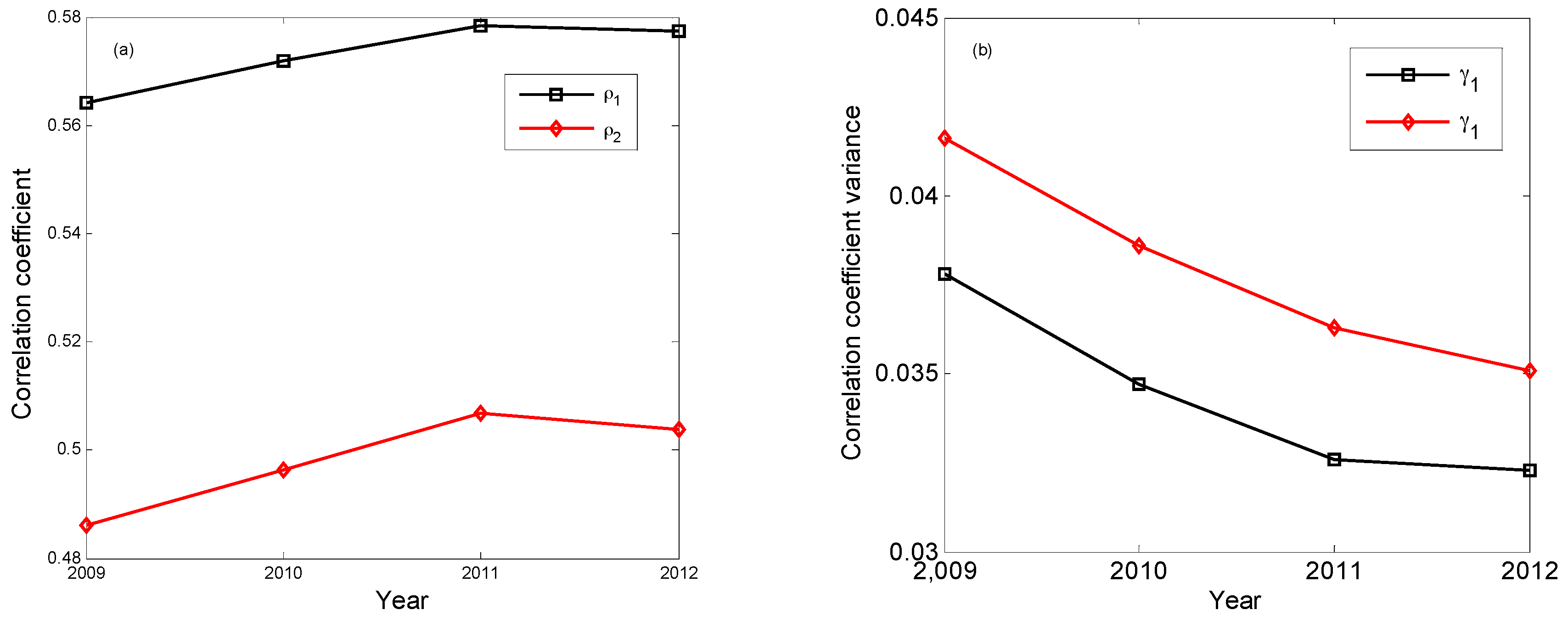
2.2.1. Selection of the Significant Correlation Coefficient
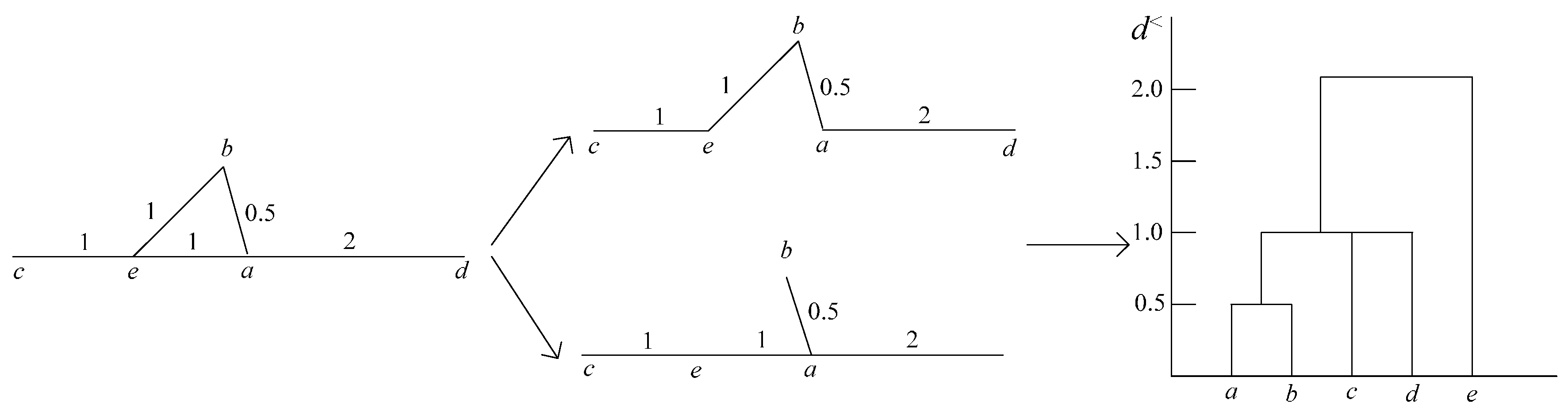
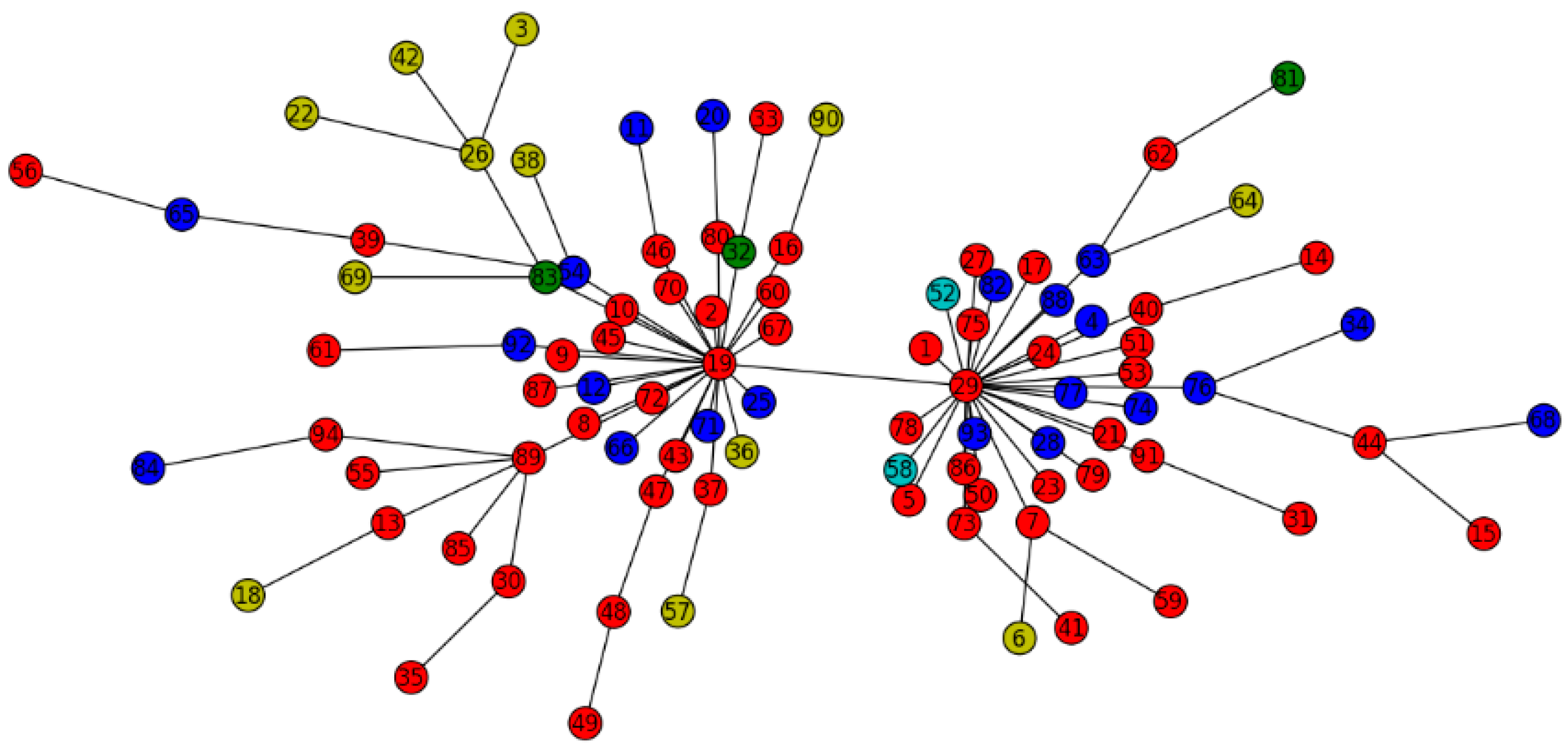
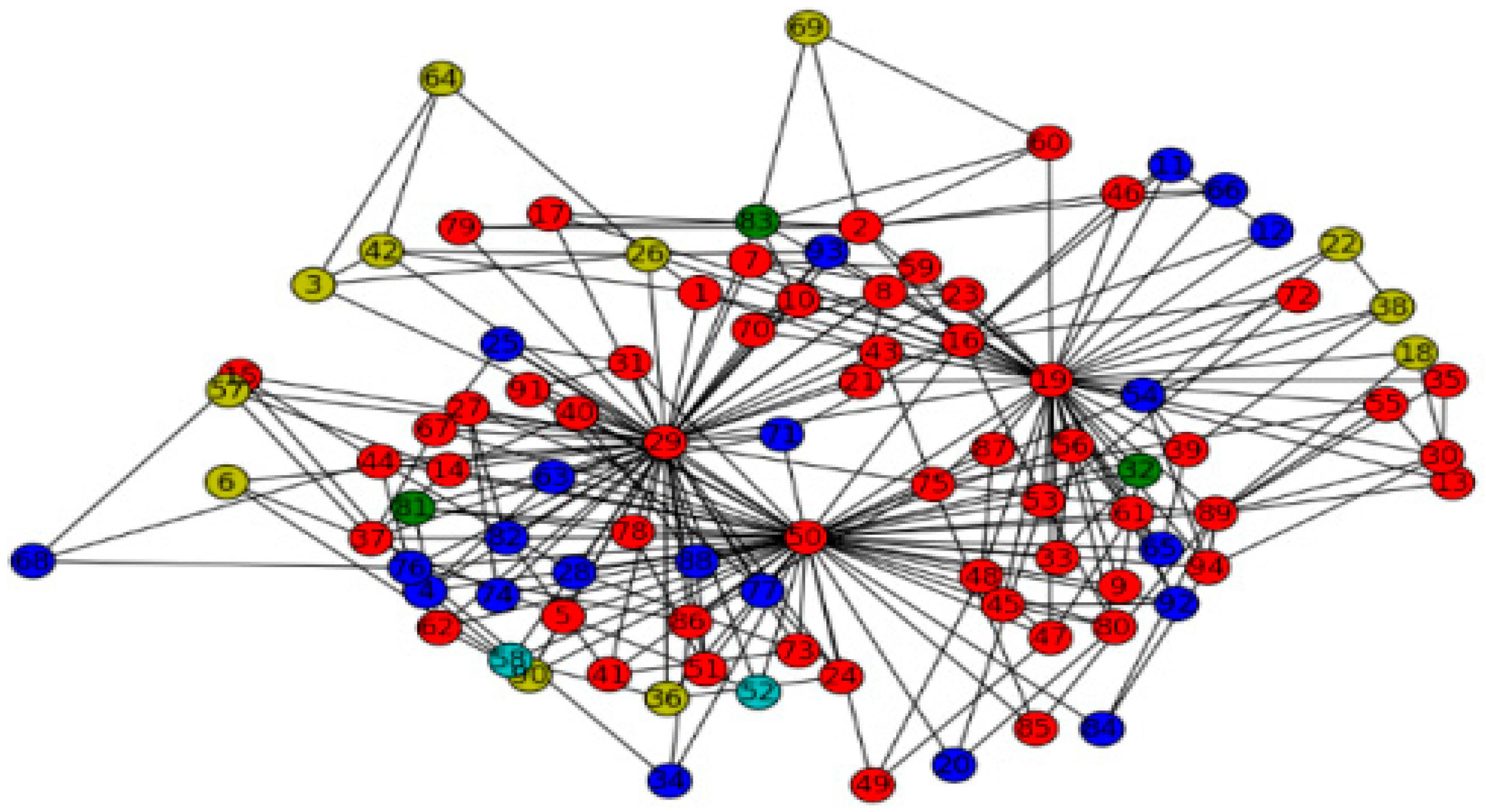
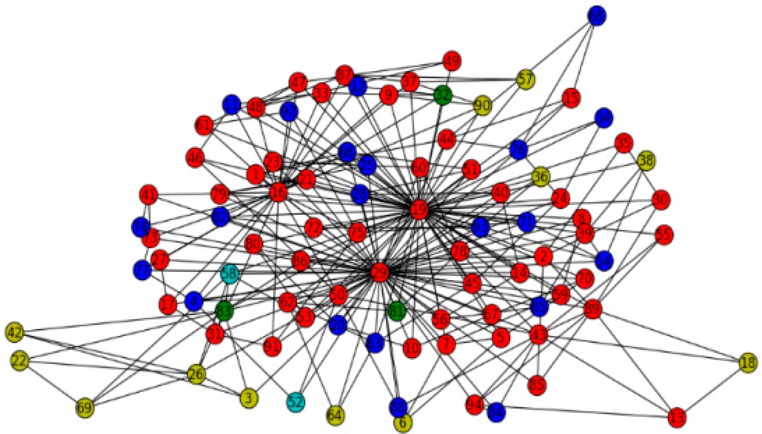
2.2.2. Network of MST and PMFG

2.2.3. Characteristic Indicators of a Network
3. Results and Discussion
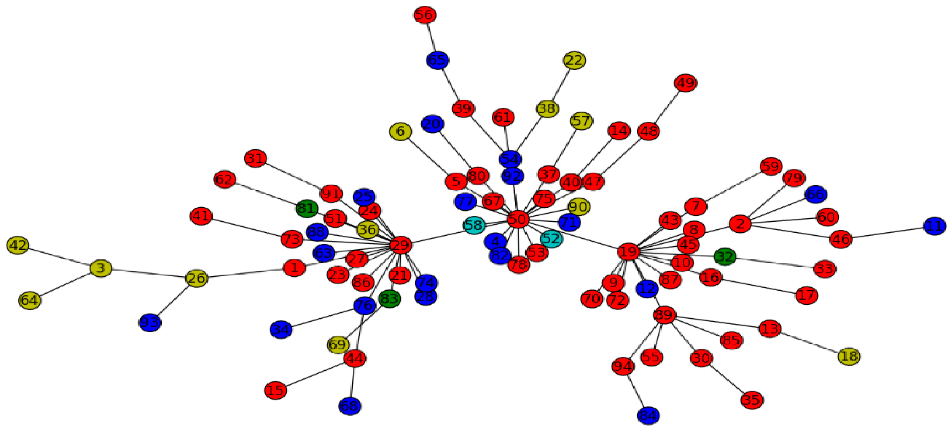
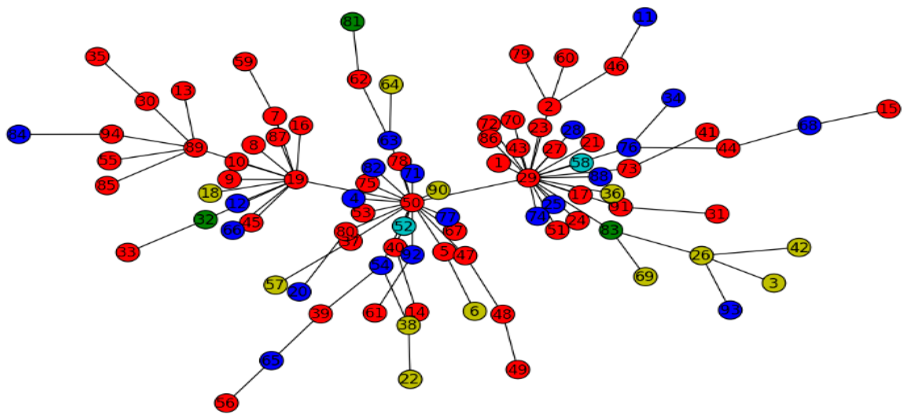
3.1. Evolution Characteristics and Strategy Identification over a Time Period


| Time Period | |||||||
|---|---|---|---|---|---|---|---|
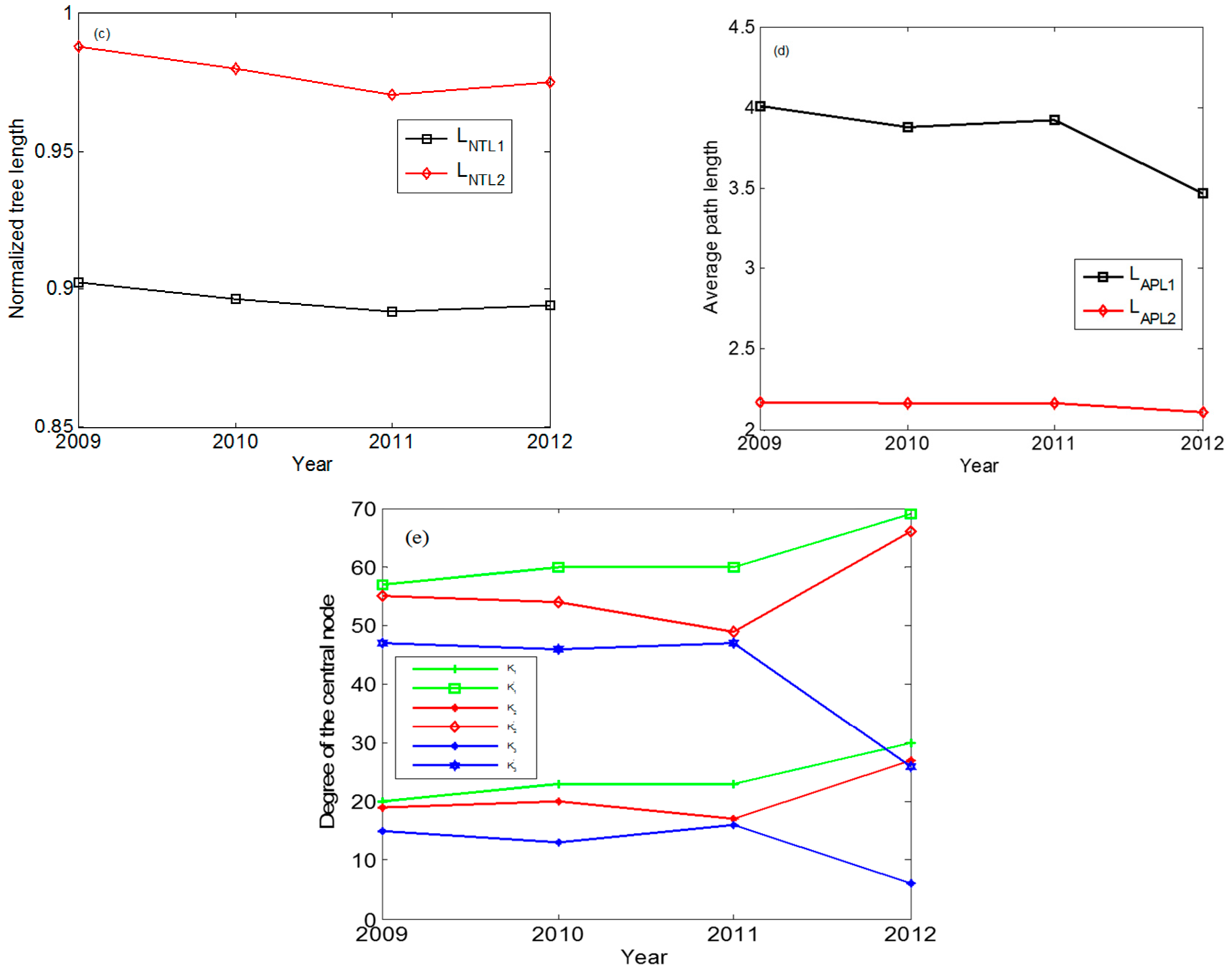
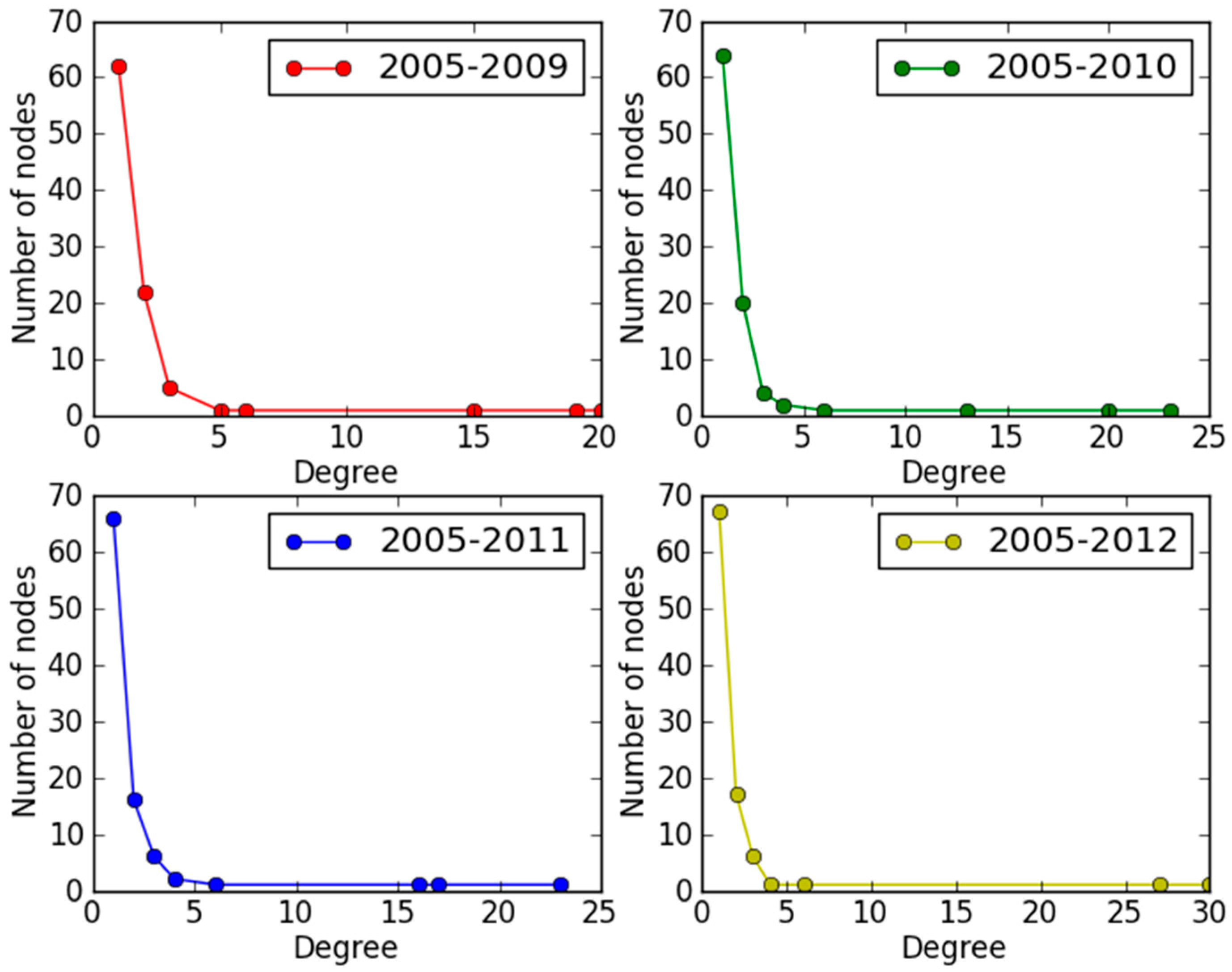
| 2005–2009 | 0.5642 | 0.0378 | 0.9025 | 4.0105 | 20(50) | 19(29) | 15(19) |
| 2005–2010 | 0.5718 | 0.0347 | 0.8964 | 3.8813 | 23(29) | 20(50) | 13(19) |
| 2005–2011 | 0.5784 | 0.0326 | 0.8916 | 3.9243 | 23(29) | 17(50) | 16(19) |
| 2005–2012 | 0.5775 | 0.0323 | 0.8940 | 3.4706 | 30(29) | 27(19) | 6(89) |
| Time period | |||||||
|---|---|---|---|---|---|---|---|
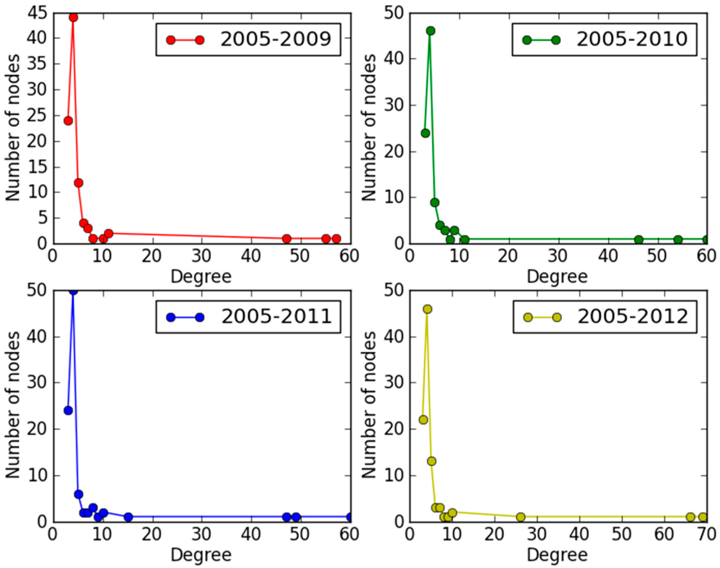
| 2005–2009 | 0.4862 | 0.0416 | 0.9879 | 2.1716 | 57(50) | 55(29) | 47(19) |
| 2005–2010 | 0.4963 | 0.0386 | 0.9796 | 2.1645 | 60(29) | 54(50) | 46(19) |
| 2005–2011 | 0.5067 | 0.0363 | 0.9703 | 2.1661 | 60(29) | 49(50) | 47(19) |
| 2005–2012 | 0.5039 | 0.0351 | 0.9750 | 2.1080 | 69(19) | 66(29) | 26(16) |


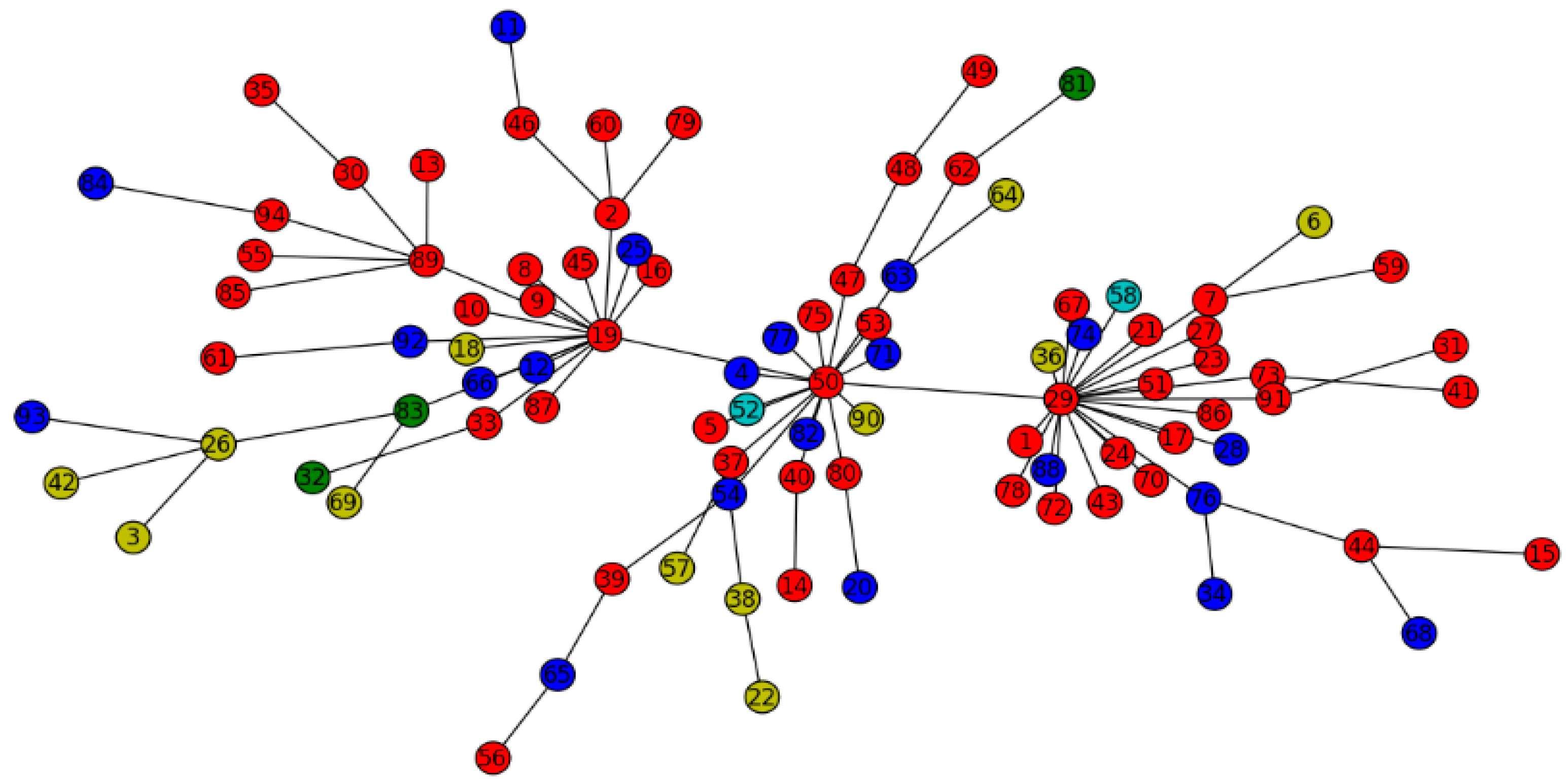
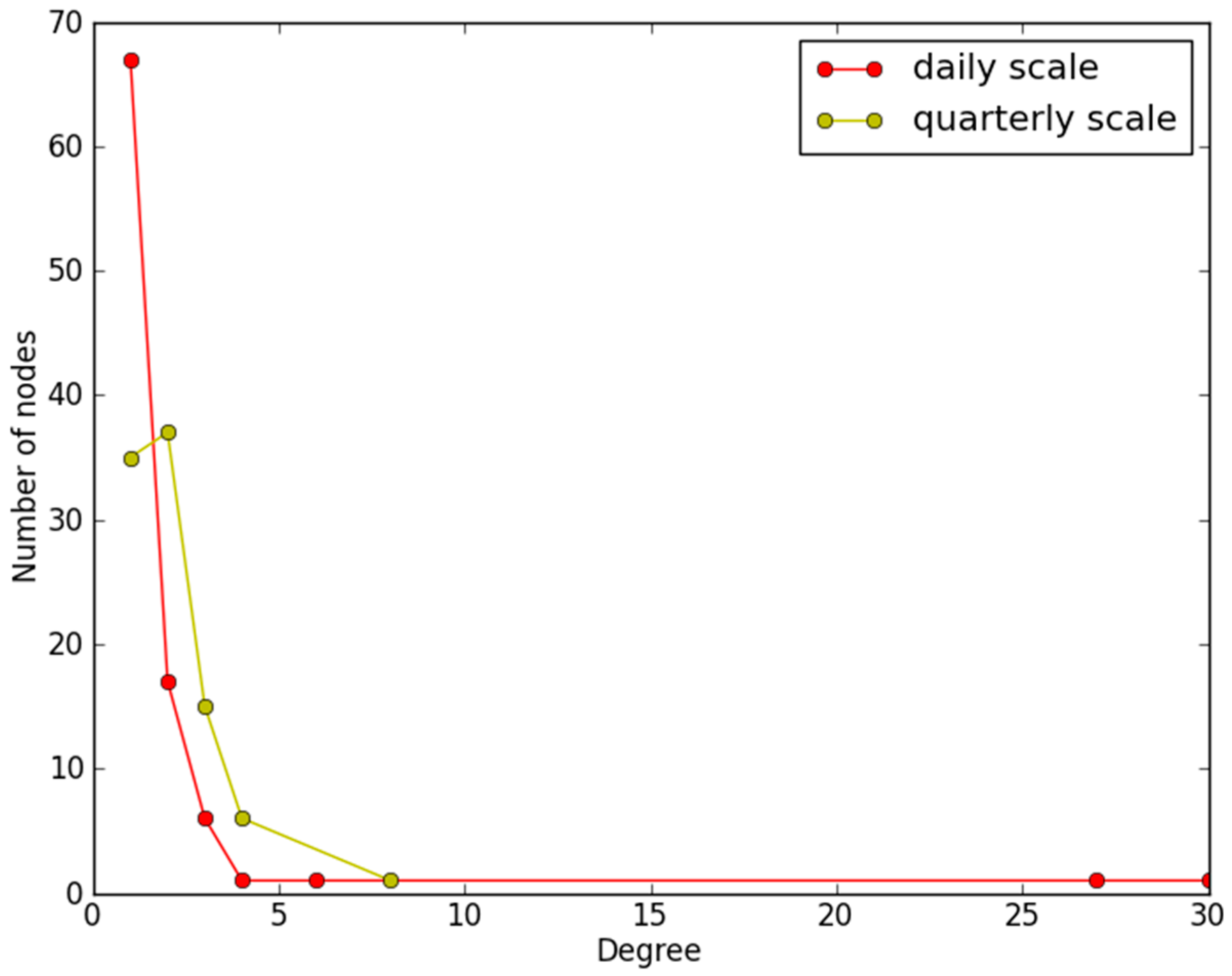
3.2. Evolution Characteristics and Strategy Identification over Timescales
| Timescale | ||||
|---|---|---|---|---|
| daily | 0.5775 | 0.03225 | 0.8940 | 3.4706 |
| weekly | 0.6631 | 0.0247 | 0.7947 | 5.2398 |
| monthly | 0.8008 | 0.0197 | 0.5943 | 8.8161 |
| quarterly | 0.9968 | 0.0003 | 0.0277 | 9.3811 |


4. Conclusions
Acknowledgments
Author Contributions
Conflicts of Interest
Appendix
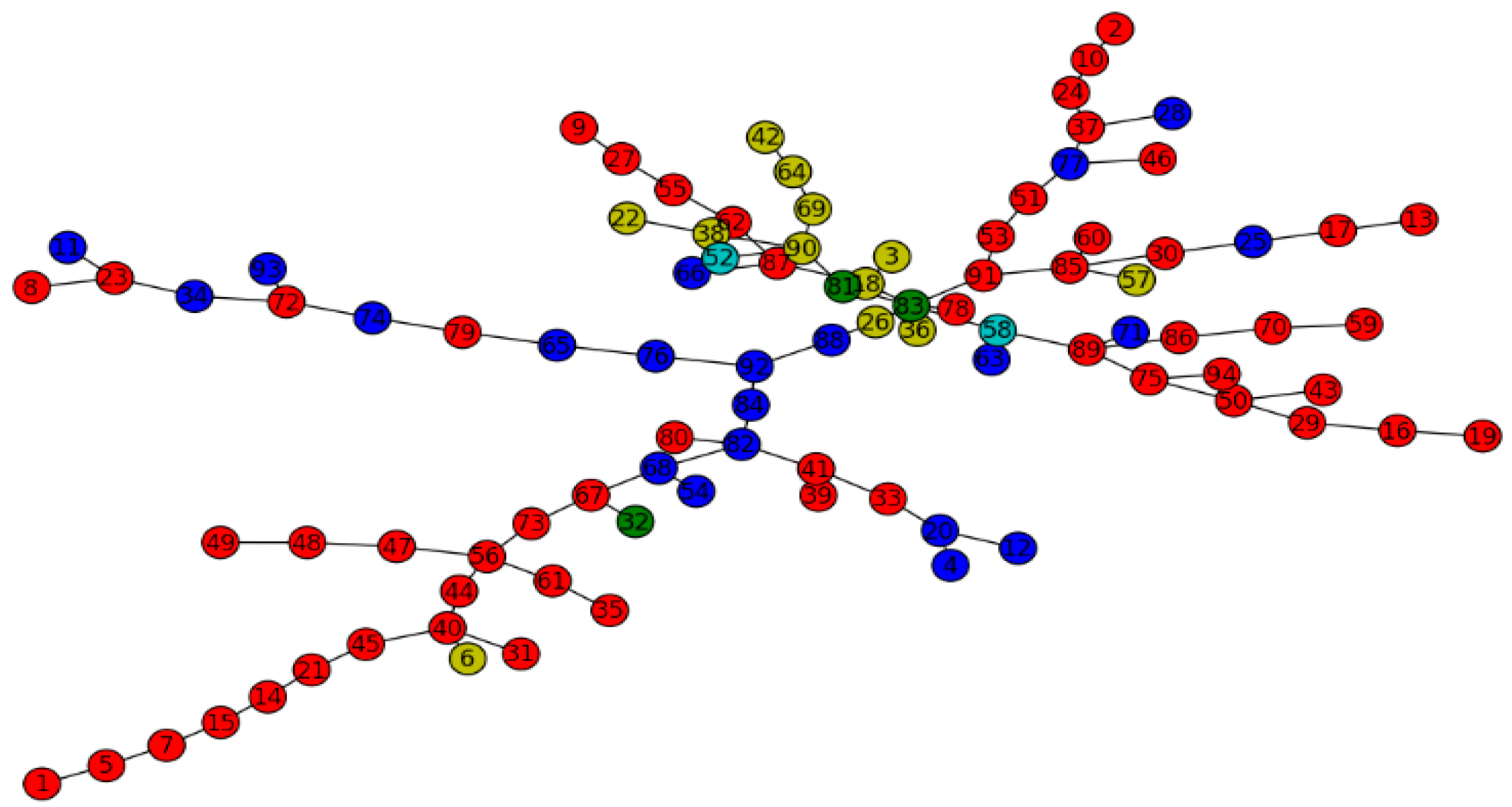
| Fund Code | Fund Name Abbreviation | Fund Type | Corresponding Code in Network (Color) | Fund Code | Fund Name Abbreviation | Fund Type | Corresponding Code in Network (Color) |
|---|---|---|---|---|---|---|---|
| 000001 | HXCZ | partial stock fund | 1 (red) | 162202 | TDZQ | partial stock fund | 48 (red) |
| 000011 | HXDP | partial stock fund | 2 (red) | 162203 | TDWD | partial stock fund | 49 (red) |
| 001001 | HXZQA/B | bond fund | 3 (yellow) | 162204 | TDJX | partial stock fund | 50 (red) |
| 002001 | HXHB | stock bond balanced fund | 4 (blue) | 180001 | YHYS | partial stock fund | 51 (red) |
| 020001 | GTJY | partial stock fund | 5 (red) | 180002 | YHBB | principal guaranteed fund | 52 (cyan) |
| 020002 | GTZQA | bond fund | 6 (yellow) | 180003 | YH88 | partial stock fund | 53 (red) |
| 020003 | GTJX | partial stock fund | 7 (red) | 200001 | CCJH | stock bond balanced fund | 54 (blue) |
| 020005 | GTJM | partial stock fund | 8 (red) | 200002 | CCJT | partial stock fund | 55 (red) |
| 040001 | HACX | partial stock fund | 9 (red) | 202001 | NFWJ | partial stock fund | 56 (red) |
| 040002 | HAAG | partial stock fund | 10 (red) | 202101 | NFBY | bond fund | 57 (yellow) |
| 040004 | HABL | stock bond balanced fund | 11 (blue) | 202202 | NFBX | principal guaranteed fund | 58 (cyan) |
| 050001 | BSZZ | stock bond balanced fund | 12 (blue) | 206001 | PHCZ | partial stock fund | 59 (red) |
| 050002 | BSYF | partial stock fund | 13 (red) | 210001 | JYYX | partial stock fund | 60 (red) |
| 050004 | BSJX | partial stock fund | 14 (red) | 213001 | BYHL | partial stock fund | 61 (red) |
| 070001 | JSCZ | partial stock fund | 15 (red) | 217001 | ZSGP | partial stock fund | 62 (red) |
| 070002 | JSZZ | partial stock fund | 16 (red) | 217002 | ZSPH | stock bond balanced fund | 63 (blue) |
| 070003 | JSWJ | partial stock fund | 17 (red) | 217003 | ZSZQA | bond fund | 64 (yellow) |
| 070005 | JSZQ | bond fund | 18 (yellow) | 217005 | ZSXF | stock bond balanced fund | 65 (blue) |
| 070006 | JSFW | partial stock fund | 19 (red) | 233001 | DMJC | stock bond balanced fund | 66 (blue) |
| 080001 | CSCZ | stock bond balanced fund | 20 (blue) | 240001 | BKXF | partial stock fund | 67 (red) |
| 090001 | DCJZ | partial stock fund | 21 (red) | 240002 | BKPZ | stock bond balanced fund | 68 (blue) |
| 090002 | DCZQA/B | bond fund | 22 (yellow) | 240003 | BKZQ | bond fund | 69 (yellow) |
| 090003 | DCLC | partial stock fund | 23 (red) | 240005 | HBCL | partial stock fund | 70 (red) |
| 090004 | DCJX | partial stock fund | 24 (red) | 255010 | WCWJ | stock bond balanced fund | 71 (blue) |
| 100016 | FGTY | stock bond balanced fund | 25 (blue) | 257010 | GLAJP | partial stock fund | 72 (red) |
| 100018 | FGTL | bond fund | 26 (yellow) | 260101 | JXGP | partial stock fund | 73 (red) |
| 100020 | FGTY | partial stock fund | 27 (red) | 260103 | JXDL | stock bond balanced fund | 74 (blue) |
| 110001 | YJPW | stock bond balanced fund | 28 (blue) | 260104 | JSZZ | partial stock fund | 75 (red) |
| 110002 | YJCL | partial stock fund | 29 (red) | 270001 | GFJF | stock bond balanced fund | 76 (blue) |
| 110003 | YJ50 | partial stock fund | 30 (red) | 270002 | GFWJ | stock bond balanced fund | 77 (blue) |
| 110005 | YJJJ | partial stock fund | 31 (red) | 288001 | HXJD | partial stock fund | 78 (red) |
| 121001 | GTRH | partial bond fund | 32 (green) | 290002 | TXXX | partial stock fund | 79 (red) |
| 121002 | GTJQ | partial stock fund | 33 (red) | 310308 | SLJX | partial stock fund | 80 (red) |
| 150103 | YHYT | stock bond balanced fund | 34 (blue) | 310318 | SLPZ | partial bond fund | 81 (green) |
| 151001 | YHWJ | partial stock fund | 35 (red) | 320001 | NAPH | stock bond balanced fund | 82 (blue) |
| 151002 | YHSY | bond fund | 36 (yellow) | 340001 | XQCJ | partial bond fund | 83 (green) |
| 160105 | NFJP | partial stock fund | 37 (red) | 350001 | TZCF | stock bond balanced fund | 84 (blue) |
| 160602 | PTZQA | bond fund | 38 (yellow) | 360001 | LHHX | partial stock fund | 85 (red) |
| 160603 | PTSY | partial stock fund | 39 (red) | 375010 | STYS | partial stock fund | 86 (red) |
| 160605 | PHZG50 | partial stock fund | 40 (red) | 398001 | ZHCZ | partial stock fund | 87 (red) |
| 161601 | XLC | partial stock fund | 41 (red) | 400001 | DFL | stock bond balanced fund | 88 (blue) |
| 161603 | RTZQA | bond fund | 42 (yellow) | 510050 | 50ETF | partial stock fund | 89 (red) |
| 161604 | RTSZ100 | partial stock fund | 43 (red) | 510080 | CSZQ | bond fund | 90 (yellow) |
| 161605 | RTLC | partial stock fund | 44 (red) | 510081 | CSJX | partial stock fund | 91 (red) |
| 161606 | RTHY | partial stock fund | 45 (red) | 519003 | HFSY | stock bond balanced fund | 92 (blue) |
| 162102 | JYZXP | partial stock fund | 46 (red) | 519011 | HFJX | stock bond balanced fund | 93 (blue) |
| 162201 | TDCZ | partial stock fund | 47 (red) | 519180 | WJ180 | partial stock fund | 94 (red) |
References
- Mantegna, R.N.; Stanley, H.E. An Introduction to Econophysics: Correlations and Complexity in Finance; Cambridge University Press: Cambridge, UK, 2000. [Google Scholar]
- Mantegna, R.N. Hierarchical structure in financial markets. Eur. Phys. J. B 1999, 5, 193–197. [Google Scholar] [CrossRef]
- Onnela, J.P.; Chakraborti, A.; Kaski, K.; Kertész, J. Dynamic asset trees and portfolio analysis. Eur. Phys. J. B 2002, 30, 285–288. [Google Scholar] [CrossRef]
- Onnela, J.P.; Chakraborti, A.; Kaski, K.; Kertész, J.; Kanto, A. Dynamics of market correlations: Taxonomy and portfolio analysis. Phys. Rev. E 2003, 68, 056110. [Google Scholar] [CrossRef] [PubMed]
- Brida, J.G.; Risso, W.A. Multidimensional minimal spanning tree: The Dow Jones case. Physica A 2008, 387, 5205–5210. [Google Scholar] [CrossRef]
- Gilmore, C.G.; Lucey, B.M.; Boscia, M. An ever-closer union? Examining the evolution of linkages of European equity markets via minimum spanning trees. Physica A 2008, 387, 6319–6329. [Google Scholar] [CrossRef]
- Jung, W.S.; Kwon, O.; Wang, F.; Kaizoji, T.; Moon, H.T.; Stanley, H.E. Group dynamics of the Japanese market. Physica A 2008, 387, 537–542. [Google Scholar] [CrossRef]
- Lee, J.; Youn, J.; Chang, W. Intraday volatility and network topological properties in the Korean Stock market. Physica A 2012, 391, 1354–1360. [Google Scholar] [CrossRef]
- Garas, A.; Argyrakis, P. Correlation study of the Athens stock exchange. Physica A 2007, 380, 399–410. [Google Scholar] [CrossRef]
- Pan, R.K.; Sinha, S. Collective behavior of stock price movements in an emerging market. Phys. Rev. E 2007, 76, 046116. [Google Scholar] [CrossRef] [PubMed]
- Emmert-Streib, F.; Dehmer, M. Influence of the time scale on the construction of Financial Networks. PLoS ONE 2010, 5, e12884. [Google Scholar] [CrossRef] [PubMed]
- Benjamin, M.T.; Thiago, R.S.; Daniel, O.C. The expectation hypothesis of interest rates and network theory: The case of Brazil. Physica A 2009, 388, 1137–1149. [Google Scholar]
- Matteo, T.D.; Aste, T.; Mantegna, R.N. An interest rates cluster analysis. Physica A 2004, 339, 181–188. [Google Scholar] [CrossRef]
- Naylor, M.J.; Rose, L.C.; Moyle, B.J. Topology of foreign exchange markets using hierarchical structure methods. Physica A 2007, 382, 199–208. [Google Scholar] [CrossRef]
- Plerou, V.; Gopikrishnan, P.; Rosenow, B.; NunesAmaral, L.A.; Guhr, T.H.; Stanley, H.E. Random matrix approach to cross correlations in financial data. Phys. Rev. E 2002, 65, 066126. [Google Scholar] [CrossRef] [PubMed]
- Tumminello, M.; Aste, T.; Matteo, T.D.; Mantegna, R.N. A tool for filtering information in complex systems. Proc. Natl. Acad. Sci. USA 2005, 102, 10421–10426. [Google Scholar] [CrossRef] [PubMed]
- Coronnello, C.; Tumminello, M.; Lillo, F.; Micciche, S.; Mantegna, R.N. Sector identification in a set of stock return time series traded at the London Stock Exchange. Acta Phys. Pol. B 2005, 36, 2653–2679. [Google Scholar]
- Tumminello, M.; Matteo, T.D.; Aste, T.; Mantegna, R.N. Correlation based networks of equity returns sampled at different time horizon. Eur. Phys. J. B 2007, 55, 209–217. [Google Scholar] [CrossRef]
- Miceli, M.; Susinno, G. Using trees to grow money. Risk 2003, 16, s11–s12. [Google Scholar]
- Miceli, M.; Susinno, G. Ultrametricity in fund of funds diversification. Physica A 2004, 344, 95–99. [Google Scholar] [CrossRef]
- Rammal, R.; Toulouse, G.; Virasoro, M.A. Ultrametricity for physicists. Rev. Mod. Phys. 1986, 58, 765–788. [Google Scholar] [CrossRef]
- Gopikrishnan, P.; Plerou, P.; Liu, Y.; Amaral, L.A.N.; Gabaix, X.; Stanley, H.E. Scaling and correlation in financial time series. Physica A 2000, 287, 362–373. [Google Scholar] [CrossRef]
- Yang, H.L.; Wan, H.; Zha, Y. Autocorrelation type, timescale and statistical property in financial time series. Physica A 2013, 392, 1681–1693. [Google Scholar] [CrossRef]
© 2015 by the authors; licensee MDPI, Basel, Switzerland. This article is an open access article distributed under the terms and conditions of the Creative Commons by Attribution (CC-BY) license (http://creativecommons.org/licenses/by/4.0/).
Share and Cite
Yang, H.; Fang, P.; Wan, H.; Liu, Y.; Lei, H. Evolution Characteristics of Complex Fund Network and Fund Strategy Identification. Entropy 2015, 17, 8073-8088. https://0-doi-org.brum.beds.ac.uk/10.3390/e17127861
Yang H, Fang P, Wan H, Liu Y, Lei H. Evolution Characteristics of Complex Fund Network and Fund Strategy Identification. Entropy. 2015; 17(12):8073-8088. https://0-doi-org.brum.beds.ac.uk/10.3390/e17127861
Chicago/Turabian StyleYang, Honglin, Penglan Fang, Hong Wan, Yucan Liu, and Hui Lei. 2015. "Evolution Characteristics of Complex Fund Network and Fund Strategy Identification" Entropy 17, no. 12: 8073-8088. https://0-doi-org.brum.beds.ac.uk/10.3390/e17127861