Entropy-Assisted Computing of Low-Dissipative Systems

Abstract

Entropy feedback is reviewed and highlighted as the guiding principle to reach extremely low dissipation. This principle is illustrated through turbulent flow simulations using the entropic lattice Boltzmann scheme.

1. Introduction

The operation of many natural and engineered systems depends crucially on their ability to function at very low dissipation rates, the lower most often the better [1]. Zero-dissipation, however, is an ideal limit which could only be reached if these systems could operate at virtually infinite processing speed. Hence, a very general question arises: how low can one keep dissipation in a given thermodynamic system?

Here we show that the ability of a specific class of fluid-kinetic systems [2,3,4] to function at a very low dissipation is dramatically enhanced by enforcing the second principle of thermodynamics in the form of an entropic feedback [5]. Through concrete examples of turbulent flows, we highlight how entropy-assisted simulation maintains the system at low viscosity, through a highly orchestrated and self-consistent interplay between local enhancement and reduction of the dissipation. Balancing of these dissipation fluctuations leads to a spatial distribution of the average effective viscosity which keeps the simulation “alive and well”. We envisage the entropy-assisted computing procedure to offer a general paradigm for the computer simulation of a wide class of low-dissipative complex phenomena, such as classical and quantum turbulence and wave propagation in active media.

2. Survival below Minimum Dissipation Threshold

The second principle of thermodynamics stands out as one of the most general and inescapable laws of physics, with profound bearings on the time evolution of virtually all natural systems [1]. In its essence, it states that any natural system is driven towards a state of maximum entropy (equilibrium), characterized by a maximum number of microscopic configurations. However, it says little about a most relevant question: how long does it take for a given system to reach its equilibrium state? This question, the heart of non-equilibrium thermodynamics, is all but academic, since most natural phenomena, life in the first place, depend on the time the system is able to borrow from temporary elusion of the second principle [1]. The rate of decay to equilibrium is measured by transport coefficients, such as kinematic viscosity, and can change widely from system to system, from seconds in an ordinary gas, to years and centuries in glassy materials.

The typical form of kinematic viscosity is given by $\nu \sim v_T^2\tau$, where $v_T=\sqrt{k_{B}T/m}$ is the thermal speed, τ a typical relaxation time. The kinematic viscosity measures the diffusivity of momentum across the system: such diffusivity results from the competition between kinetic energy, which sustains the free motion of molecules, and potential energy, which controls their interactions (collisions). Kinetic energy drives the system out of equilibrium, while molecular collisions pull it back to a local equilibrium, in which entropy is locally maximized (Boltzmann’s H-theorem) [6,7,8]. Thus, a low-viscous fluid is not one with nearly no collisions, but one where collisions are so frequent and effective that they inhibit any migration of momentum from place to place, which is the source of macroscopic dissipation. From the above argument, it is seen that zero-viscosity is a mirage because it would imply instantaneous relaxation, i.e., $\tau \to 0$. Given that strictly zero-viscosity is a chimera in a real (finite-speed) world, a natural question arises: what is the minimum dissipation which can be sustained by a given physical system? While the answer depends on the specific system in mind, here we shall focus on discrete dynamical systems, i.e., featuring a fundamental minimal length scale a and minimal time scale h.

For the case of simulated fluids, for instance, the condition is that the smallest coherent structures (eddies) capable of surviving dissipation be resolved by the discrete grid, i.e., $l_{\mathrm{K}}>a$, where $l_{\mathrm{K}}\sim L/{\mathrm{Re}}^{3/4}$ is the so-called Kolmogorov’s length [9], the smallest active scale in the game and $\mathrm{Re}=UL/\nu$ is the Reynolds number, i.e., the ratio of nonlinear energy transfer to dissipation, for a fluid moving at a macroscopic speed U on a domain of macroscopic size L. As a result, the minimal viscosity is given by ${\nu }_{\min }=(u/N^{1/3}){\nu }_l$, where $N=L/a$ is the grid size, $u\equiv U/U_{\mathrm{l}}$, $U_{\mathrm{l}}=a/h$ and ${\nu }_{\mathrm{l}}=a^2/h$ being the natural lattice speed and lattice viscosity, respectively. Given that $u<1$ for reasons of numerical stability, we see that the minimal viscosity is always smaller than the lattice viscosity, the ratio of the two decreasing like $1/N^{1/3}$, so that the minimum viscosity can be brought to zero only in the continuum limit $N\to \infty$. Another face of the same chimera. The message is that fluids cannot support viscosity below their minimum bound ${\nu }_{\min }$. Breaking such constraint leads to two basic scenarios: a mild reaction (loss of accuracy), whereby the resolved eddies, $l>a$, still survive, although with a corrupted dynamics, the degree of corruption increasing as they approach a. The second, more dramatic, possibility is loss of realizability: the system develops disruptive instabilities, typically in the form of an uncontrolled growth of the smallest eddies. This is nothing short of a survival problem, except that it concerns a discrete dynamical system. From the practical point of view, the art of keeping the system alive and well in the forbidden regime $\nu <{\nu }_{\min }$ is known as turbulence modeling, a topic of utmost practical and conceptual importance. Essentially, the idea is to replace the nominal viscosity with an effective one, representing the effects of unresolved eddies as “random” collisions on the resolved ones. This picture explicitly draws upon an analogy with kinetic theory, where there is a clear scale separation between molecular and hydrodynamic degrees of freedom. Turbulence, on the contrary, features a continuum spectrum of scales, hence the notion of eddy viscosity, although very useful, still resists a rigorous justification.

3. Minimum Viscosity in Discrete Phase-Space-Time

However, a modern formulation of continuum fluid mechanics in a form which explicitly ingrains the discreteness of space-time is known as the lattice Boltzmann equation [4]

$$f_i(x+c_{i}h;t+h)=f_i^{\prime }\equiv \left(1-\frac{h}{2\tau }\right)f_i(x,t)+\left(\frac{h}{2\tau }\right)f_i^{\mathrm{mirr}}(x,t)$$

(1)

In the above $f_i$ is the probability of finding a “particle” at position x in the lattice at time t, moving with discrete velocity $c_i$ along b lattice links; $f_i^{\mathrm{mirr}}$ is the so-called mirror state. In the simplest case [4], it is taken as $f_i^{\mathrm{mirr}}=2f_i^{\mathrm{eq}}-f_i$, with $f_i^{\mathrm{eq}}$ the local equilibrium, which is a universal non-linear function of the local order parameters. For standard fluids, these are the fluid density $n(x,t)={\sum }_i{f}_i(x,t)$ and velocity $u(x,t)=n^{-1}{\sum }_i{c}_i{f}_i(x,t)$. The left-hand side of Equation (1) represents the free-streaming step, while the right-hand side describes the interactions among the discrete populations $f_i$ at each given lattice site. On condition that the lattice obeys proper symmetries, the lattice Boltzmann Equation (1) reproduces fluid dynamics with the viscosity

$$\nu \sim \left(\frac{\tau }{h}-\frac{1}{2}\right){\nu }_{\mathrm{l}}$$

(2)

The negative shift, $-1/2$ in Equation (2) is crucial; indeed, if only in principle, it permits to achieve zero viscosity in the limit $\tau \to h/2$, i.e., without sending $\tau \to 0$, unlike in the continuum. This negative shift is the result of the broken time-symmetry, which contributes a negative viscosity (sometimes called propagation viscosity) to the overall momentum diffusivity, besides the conventional contribution due to the collisional relaxation. Thus, in a discrete world, the viscosity receives contributions from both dynamical steps of the kinetic description: free streaming and collisions. They carry opposite signs, hence, if only in principle, they can cancel each other, leaving the time step and relaxation time both finite. This property, typically regarded as a very useful numerical artifact, has played a major role in the lattice Boltzmann simulation of a variety of complex flows, and most notably turbulent ones [10].

Amazingly, suitably designed discrete kinetic systems keep describing correct fluid behavior several orders of magnitude below the hydrodynamic minimum viscosity bounds mentioned earlier in this paper. How come the minimal viscosity can be eluded by several orders of magnitude?

The key is the second principle in fully discrete setting. Indeed, the lattice Boltzmann Equation (1) is compatible with a discrete-time H-theorem, based on the H-function (negative of the entropy), $H\left[f\right]={\sum }_i{f}_{i}ln(f_i/w_i)$, where $w_i$ are suitable positive-definite weights. Lattice Boltzmann systems equipped with the H-theorem are known as entropic [5] and function on a feedback mechanism, whereby the local relaxation τ is adjusted in space and time, so as to secure the entropic bound, $H\left[f^{\prime }\right]\le H\left[f\right]$, where f and $f^{\prime }$ are the pre- and post-collisional states, respectively.

The working principle is explained in Figure 1 and amounts to using in Equation (1) the entropy-supervised mirror state $f_i^{\mathrm{mirr}}=(1-\alpha )f_i+\alpha f^{\mathrm{eq}}$, where the stretch α is found from the isentropic constraint, $H\left[f^{\mathrm{mirr}}\right]=H\left[f\right]$. This can be interpreted as the effective viscosity,

$${\nu }_{\mathrm{eff}}\sim \left(\frac{{\tau }_{\mathrm{eff}}}{h}-\frac{1}{2}\right){\nu }_{\mathrm{l}}$$

(3)

with the effective relaxation time, ${\tau }_{\mathrm{eff}}=2\tau /\alpha$. The entropy-assisted computation thus informs the pre-collision state f about its isentropic mirror $f^{\mathrm{mirr}}$ and stipulates the single condition that the second law is respected by the post-collision state $f^{\prime }$. Whenever non-equilibrium effects become strong enough to endanger realizability, the entropic constraint adjusts the relaxation time so as to secure compliance with the second principle. This feedback is self-activated “on demand”, i.e., only whenever and wherever the need arises. And when the danger is gone, most elegantly, the entropic feedback, leaves the stage unsolicited. The second principle decides by itself: sometimes viscosity is increased (${\nu }_{\mathrm{eff}}>\nu$) to smooth out sharp features, sometimes it is reduced (${\nu }_{\mathrm{eff}}<\nu$) to sharpen the dying ones. In the most demanding cases, the effective viscosity may even drop negative (${\tau }_{\mathrm{eff}}<h/2$) to promote local instabilities and sustain the system against dissipative death. The effective viscosity self-adapts to the actual state of turbulence to literally protect it against defective evolution and disruptive instabilities.

In Figure 2 we illustrate the above by the vorticity field of a flow past a circular cylinder at $\mathrm{Re}\sim 3300$, in which many active scales of motion are visible. The Reynolds number, $\mathrm{Re}=UD/\nu$, is based on the diameter of the cylinder, which is here taken as $D=30a$, while the mean flow velocity is $U=0.03(a/h)$, corresponding to a viscosity $\nu =UD/\mathrm{Re}\sim 2.7\times {10}^{-4}(a^2/h)$. With these parameters, the minimum viscosity is ${\nu }_{\min }=0.03/{30}^{1/3}\sim 0.01(a^2/h)$, so that $\nu /{\nu }_{\min }\sim 1/40$. The flow structures in Figure 2a are colored with the effective viscosity, normalized as $R=({\nu }_{\mathrm{eff}}-\nu )/\nu$. The high quality of resolution of the flow structures (vortex tubes, tangles etc.) is maintained by a concerted action of dampers ($R>0$) and promoters ($R<0$). The tiniest structures would not be able to survive unless the effective viscosity is enabled to go negative from time to time, in order to compensate for over-dissipation and “regenerate” small scale structures otherwise doomed by over-damping. Also to be noted (Figure 2b) is the spottiness of the effective viscosity, with a highly fine-grained mixing of dampers and promoters.

Figure 1. Entropy-assisted computing. The initial state f is over-relaxed to the state $f^{\prime }$ with the entropy function H value strictly below the value at the entropy mirror state $f^{\mathrm{mirr}}$. The zigzag trajectory of over-relaxations eventually ends up at the bottom of the well—at the equilibrium $f^{\mathrm{eq}}$.

Figure 1. Entropy-assisted computing. The initial state f is over-relaxed to the state $f^{\prime }$ with the entropy function H value strictly below the value at the entropy mirror state $f^{\mathrm{mirr}}$. The zigzag trajectory of over-relaxations eventually ends up at the bottom of the well—at the equilibrium $f^{\mathrm{eq}}$.

Figure 2. (a) Turbulent flow generated by a round cylinder. Snapshot of the vorticity iso-surfaces are shown, colored with the effective viscosity. Blue: $R>0$ (dampers); Red/Yellow: $R<0$ (promoters). The interplay between the dampers and promoters along each vortex tube is clearly seen. (b) Snapshot of the intertwining of dampers ($R>0$, blue) and promoters ($R<0$, red). Essential dampers ($R>1.5$) and promoters ($R<-0.6$) are shown. The entropic feedback is concentrated in the region behind the obstacle, where the transition to turbulence occurs. Gray background: Vorticity.

Figure 2. (a) Turbulent flow generated by a round cylinder. Snapshot of the vorticity iso-surfaces are shown, colored with the effective viscosity. Blue: $R>0$ (dampers); Red/Yellow: $R<0$ (promoters). The interplay between the dampers and promoters along each vortex tube is clearly seen. (b) Snapshot of the intertwining of dampers ($R>0$, blue) and promoters ($R<0$, red). Essential dampers ($R>1.5$) and promoters ($R<-0.6$) are shown. The entropic feedback is concentrated in the region behind the obstacle, where the transition to turbulence occurs. Gray background: Vorticity.

All of the above configures a very elegant preemptive scenario which we can take as the hallmark of entropic computing: very attentive “guardian angels”. Amazingly, the spatial pattern of the time-averaged effective viscosity shown in Figure 3 resembles indeed a “guardian angel”, protecting the system against numerical crisis!

Figure 3. Distribution of the time-averaged normalized effective viscosity $R=({\nu }_{\mathrm{eff}}-\nu )/\nu$ at the mid-section of the flow past a round cylinder. Red/Yellow: Promoters ($R<0$); Blue: Dampers ($R>0$); Green: Nominal ($R=0$). While the snapshot in Figure 2 demonstrates a larger variation of the effective viscosity, the time-average picture is much milder: most of the activity (strongest damping neighboring the strongest promotion) is concentrated at and around the twin shear layers, just behind the cylinder. In the rest of the domain, the deviation of the effective viscosity from its nominal value is less than a fraction of a percent.

Figure 3. Distribution of the time-averaged normalized effective viscosity $R=({\nu }_{\mathrm{eff}}-\nu )/\nu$ at the mid-section of the flow past a round cylinder. Red/Yellow: Promoters ($R<0$); Blue: Dampers ($R>0$); Green: Nominal ($R=0$). While the snapshot in Figure 2 demonstrates a larger variation of the effective viscosity, the time-average picture is much milder: most of the activity (strongest damping neighboring the strongest promotion) is concentrated at and around the twin shear layers, just behind the cylinder. In the rest of the domain, the deviation of the effective viscosity from its nominal value is less than a fraction of a percent.

4. Entropic Lattice Boltzmann Algorithm

Here we describe the essentials of the simulation method used above. In the entropic lattice Boltzmann scheme, populations associated with the discrete velocities $c_i$ evolve according to (1). The local equilibrium $f_i^{\mathrm{eq}}$ was found by minimizing the entropy function $H\left[f\right]$. The entropic mirror state $f_i^{\mathrm{mirr}}=(1-\alpha )f_i+\alpha f^{\mathrm{eq}}$ is specified by the stretch α, which is computed as the positive root of the entropy condition: $H[f+\alpha (f^{\mathrm{eq}}-f)]=H\left[f\right]$. Whenever the simulation is resolved at a particular grid node x, the stretch α becomes fixed automatically to the value $\alpha =2$ at that node, and the effective viscosity ${\nu }_{\mathrm{eff}}$ (3) reduces to the nominal viscosity $\nu$ (2). The stretch was obtained numerically at each grid point using Newton-Raphson method. For the simulation presented above, we used the lattice with $b=15$ discrete velocities [11]. Apart from an entropy-supported kinetic equation, we require augmenting boundary conditions that are capable of simulating both resolved and under-resolved flows. Existing boundary conditions such as the bounce-back scheme [4], provide reliable results for resolved simulations but with reducing grid sizes and increasing the Reynolds number, the quality of the simulations is lost due to shock-like instabilities generated at the walls. Hence, we used here the recently proposed Tamm–Mott-Smith boundary condition [12] for circumventing these instabilities. Entropy-supported kinetic Equation (1) provides reliable simulations for any choice of lattice and flow velocity as long as the Mach number remains small. Armed with stable boundary condition, the present scheme was extensively tested for various flow setups such as decaying turbulence ($\nu /{\nu }_{\min }\sim {10}^{-4}$) [13], turbulent channel ($\nu /{\nu }_{\min }\sim {10}^{-3}$) [12], grid generated turbulence ($\nu /{\nu }_{\min }\sim {10}^{-3}$), flow past an airfoil ($\nu /{\nu }_{\min }\sim {10}^{-4}$) and others. For the particular simulation of the flow past a circular cylinder presented in Figure 2 and Figure 3, we used a computational domain that is $9D$ long in the span-wise direction, $35D$ along in the stream-wise direction with $10D$ upstream of the cylinder and $25D$ downstream of it; along vertical direction the domain was $21D$ long with cylinder axis in the mid-plane. The cylinder was resolved with the diameter $D=30$ grid points. Apart from the simulation of turbulent flows, the entropy feedback has significantly improved stability of thermal flows with temperature gradients [14], multiphase flows [15] and other fluid dynamics problems. This gives us strong confidence that entropy-guidance can be extended to other low-dissipative physical systems.

5. ELBM: Questions and Answers

Here we answer some typical questions to the entropic lattice Boltzmann method (ELBM) reviewed above. For the sake of convenience, we rewrite the ELBM equation setting the time step $h=1$:

$$f_i(x+c_i,t+1)\equiv f_i^{\prime }=(1-\beta )f_i(x,t)+\beta f_i^{\mathrm{mirr}}(x,t)$$

(4)

where $\beta \in [0,1]$, while the entropic mirror state $f^{\mathrm{mirr}}$ is

$$f_i^{\mathrm{mirr}}=f_i+\alpha (f_i^{\mathrm{eq}}-f_i)$$

(5)

The stretch α is defined by the entropy balance between the pre-collision state f and the mirror state $f^{\mathrm{mirr}}$,

$$H\left(f^{\mathrm{mirr}}\right)=H\left(f\right)$$

(6)

A discrete-time H-theorem states: If the non-trivial solution α exists for the entropy balance (6), then the total entropy $\overline{H}\left(t\right)={\sum }_{\mathit{x}}H\left(f(\mathit{x},t)\right)$ is not increasing, $\overline{H}(t+1)\le \overline{H}\left(t\right)$. Note that the validity of the H-theorem requires not just the equilibrium to be evaluated through the minimization of H but also, and most importantly, the fulfillment of the entropy balance condition (6).

• Is the entropic feedback in ELBM a stabilizing technique or a physically sound subgrid-scale model for turbulence?
  A: The ELBM should be viewed as a built-in subgrid model rather than a mere stabilization technique. Stabilization in ELBM is a by-product of the discrete-time H-theorem. Instead of a mere addition of artificial viscosity, the ELBM allows the effective viscosity to fluctuate around the target value $\nu$. In order to clarify this point, note a few general features of the entropic stretch α.

  • Over-relaxation: Thanks to convexity of the entropy function, the solution to Equation (6) always leads to over-relaxation, $\alpha >1$;
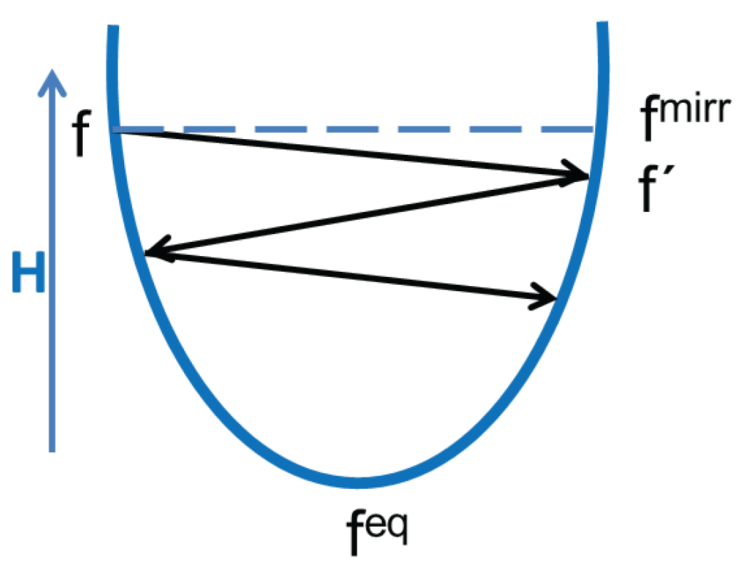
  • Duality: Let f be a population vector, and $f\left(\alpha \right)\equiv f+\alpha (f^{\mathrm{eq}}-f)$ its entropic mirror state, with the same value of the entropy, $H\left(f\right(\alpha \left)\right)=H\left(f\right)$. If the entropy estimate is applied to $f\left(\alpha \right)$ instead of f, then the initial state is recovered in the form $f=f\left(\alpha \right)+{\alpha }^{*}(f^{\mathrm{eq}}-f\left(\alpha \right))$, with another stretch ${\alpha }^{*}>1$ which satisfies a duality relation:

    $${\alpha }^{*}\alpha ={\alpha }^{*}+\alpha .$$

    (7)

    Equation (7) implies that whenever $\alpha \lessgtr 2$, the opposite holds for the dual, ${\alpha }^{*}\gtrless 2$.
  • Hydrodynamic limit: whenever the simulation is resolved (populations stay close to the local equilibrium), the stretch α tends to the fixed value $\alpha =2$ (and so does also the dual stretch, ${\alpha }^{*}=2$, according to (7)). Then ELBM self-consistently becomes equivalent to the lattice Bhatnagar–Gross–Krook (LBGK) equation ($\alpha =2$) and recovers the Navier-Stokes equations with the kinematic viscosity,

    $$\nu =c_{\mathrm{s}}^2\left(\frac{1}{2\beta }-\frac{1}{2}\right)$$

    (8)

    where $c_{\mathrm{s}}$ is speed of sound (a $O\left(1\right)$ lattice-dependent constant).
    Note that the above is a direct implication of the built-in H-theorem. Indeed, the resolved simulation, at the kinetic level, is characterized by the fact that all populations are asymptotically close to the local equilibrium. Then, the entropy function becomes well represented by its second-order approximation: at fixed locally conserved fields (density and momentum here), if $\delta f=f-f^{\mathrm{eq}}$, $|\delta f/f^{\mathrm{eq}}|\ll 1$, then $H\left(f\right)\approx H^{\mathrm{eq}}+(1/2){\sum }_i\delta f_i^2/f_i^{\mathrm{eq}}$. The levels of the entropy are then asymptotically close to the levels of the above quadratic form. It is under such condition that the entropy estimate (6) results in $\alpha =2$. Note that the standard Chapman–Enskog approximation is valid under precisely the same condition of closeness to the local equilibrium, thereby the viscosity $\nu$ is the same for both ELBM and LBGK.
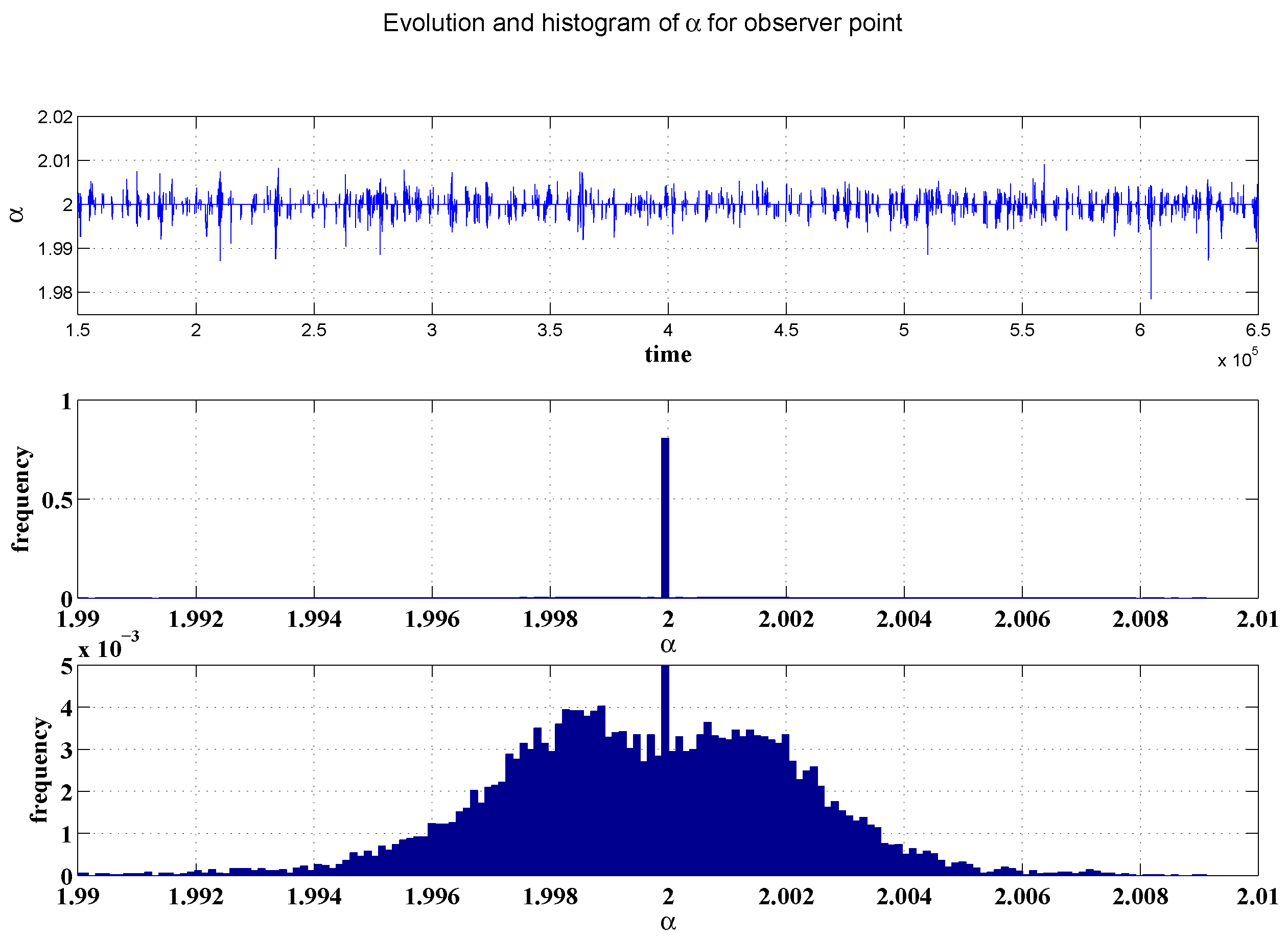
  • Effective viscosity and self-averaging: The effective viscosity in the above notation reads,

    $${\nu }_{\mathrm{eff}}=c_{\mathrm{s}}^2\left(\frac{1}{\alpha \beta }-\frac{1}{2}\right)$$

    (9)

    Depending on the outcome for stretch α, the effective viscosity ${\nu }_{\mathrm{eff}}\left(\alpha \beta \right)$ is larger than the viscosity $\nu \equiv {\nu }_{\mathrm{eff}}\left(2\beta \right)$ if $\alpha <2$, and it is smaller than $\nu$ if $\alpha >2$. In the first case, the (larger) effective viscosity leads to smoothing the velocity gradient at the given node, while in the second case, the smaller viscosity leads to a sharpening of the velocity gradient. Note that, when $\beta \to 1$ (vanishing viscosity $\nu \to 0$), the effective viscosity (9) can drop to even negative values if $\alpha >2$. This asymmetry between the over-relaxation being “shorter” ($\alpha <2$) or “longer” ($\alpha >2$) than the LBGK over-relaxation $\alpha =2$ is the crucial implication of the compliance with the H-theorem: even if the effective viscosity becomes negative at some lattice nodes, this does not lead to numerical instability because even in that case the H-theorem (and the proper behavior of the total entropy) remains valid.
    Parameterization with the effective viscosity ${\nu }_{\mathrm{eff}}\left(\alpha \beta \right)$ can be seen as an alternative to the parameterization with the over-relaxation α. Let us note that, if a pair $\{\alpha ,{\alpha }^{*}\}$ is connected by the duality relation (7), then the mean value of the corresponding effective viscosity is equal to the viscosity (8),

    $$\frac{{\nu }_{\mathrm{eff}}\left(\alpha \beta \right)+{\nu }_{\mathrm{eff}}\left({\alpha }^{*}\beta \right)}{2}={\nu }_{\mathrm{eff}}\left(2\beta \right)\equiv \nu$$

    (10)

    The relation (10) is termed self-averaging, and provides important albeit heuristic argument that the averaged-in-time effective viscosity in ELBM simulation is close to the viscosity $\nu$. In other words, we expect that it is only the matter of resolution that the average effective viscosity deviates from $\nu$. This assertion, while not rigorous, is supported by simulation (see Figure 3). The rapid fluctuations of the stretch α around $\alpha =2$ at a given monitoring point chosen at random in the simulation domain are clearly seen in Figure 4.

Figure 4. Top: History of the entropic strech α at a monitoring point; Middle: Histogram of α; Bottom: Close-up of the hystogram around the dominant value $\alpha =2$.

Figure 4. Top: History of the entropic strech α at a monitoring point; Middle: Histogram of α; Bottom: Close-up of the hystogram around the dominant value $\alpha =2$.

• In summary, the ELBGK exploits the self-adaptive mechanism of effective viscosity by choosing automatically the over-relaxation α at each node to guarantee the H-theorem at all sites and all discrete time-steps. When the grid is coarsened, over-relaxation α becomes “smeared” in an interval, $[{\alpha }_{\min },{\alpha }_{\max }]$, with $1<{\alpha }_{min}<2$, and ${\alpha }_{max}>2$. The self-adapted over-relaxation set up by (6), results in two oppositely directed effects: if $\alpha <2$, the effective viscosity is larger than $\nu$, and the ELBM will tend to smoothen any flow perturbation. On the other hand, if $\alpha >2$, the flow perturbation is enhanced (effective viscosity is smaller than $\nu$). In ELBM simulations, these two effects act simultaneously on various nodes, with the net effect combining stabilization (through smoothing, $\alpha <2$) with the preservation of the resolution (through sharpening, $\alpha >2$). Note that, as $\beta \to 1$, the effective viscosity can even drop to negative values when $\alpha >2$. This, however, does not lead to instabilities as the total entropy balance remains under control by the discrete-time H-theorem. This all is very different from a conventional perspective on “eddy viscosity” turbulence modeling, and it is not surprising that ELBM does not reduce to familiar large eddy simulation (LES) models [16].

2.

What is the relation of ELBM to the entropic stabilizing techniques proposed in CFD?

A: During the last four decades numerous entropic stabilizing techniques have been proposed in computational fluid dynamics (CFD) (see, e.g., Refs [17,18,19,20,21,22,23,24,25] and references therein). The idea behind is, roughly speaking, to maintain an appropriate amount of artificial viscosity through the analysis of discretization of the entropy balance (physical or artificial). In this regards, ELBM is based on a different premise: it applies to strictly discrete systems (in velocity-space-time), and the discrete-time H-theorem does not reduce to the estimate of the entropy production (cf., e.g., [26]).

3.

How ELBM performs in comparison to other stabilizing techniques proposed for LBM?

A: The closest analog of the conventional stabilization techniques in the LBM setting is perhaps the method of entropic limiters [27,28,29]. The idea behind is to measure the closeness of the pre-collision state to the corresponding local equilibrium (in the sense of the entropy difference), and to apply equilibration instead of over-relaxation if the difference exceeds a user-defined threshold. This is similar to conventional artificial viscosity stabilization techniques in CFD. Various versions of limiters were considered [27,28,29]. The authors of [29] claimed that entropic limiters “perform better” than ELBM.

4.

What is the main numerical mechanism promoting stability in ELBM?

A: Stability is promoted by the discrete-time H-theorem. Note that the implication of the H-theorem in the presence of the over-relaxation allows post-collision distributions to be both closer to the equilibrium than the LBGK outcome ($\alpha <2$) or further away from the equilibrium ($\alpha >2$). It must be noted that, in principle, for some pre-collision states, the corresponding entropic mirror state may not exist (and hence no entropy balance is possible). However, this happens beyond the domain of validity of the lattice Boltzmann models, and is of no concern in practice. In particular, pathological cases (no solution for α) occur in none of the simulations referred to in this paper.

5.

Very recently, in Ref. [30], Karlin et al. presented a new entropic stabilizer for LB schemes. How is it different from the ELBM?

A: ELBM is based on the discrete-time H-theorem which is imposed in a rather “orthodox” manner through the entropy balance condition (6) for the over-relaxation. A different realization of the entropic control was introduced recently by three of the present authors in [30] (we refer to this as KBC model). The idea is to replace the entropic over-relaxation on all the non-conserved moments as it is done in ELBM by a combination of the standard (unsupervised) over-relaxation of the stresses with the proper equilibration of the rest of the non-conserved moments. More specifically, if we write a moment representation of the populations, $f_i=k_i+s_i+h_i$, where $k_i$ is the contribution of locally conserved fields, $s_i$ are the stresses and $h_i$ are the remaining higher-order moments, then the mirror state for KBC models reads,

$$f_i^{\mathrm{mirr}}=k_i+[2s_i^{\mathrm{eq}}-s_i]+\left[(1-\gamma )h_i+\gamma h_i^{\mathrm{eq}}\right]$$

(11)

where $\gamma$ is the entropic stabilizer which is found by minimizing the entropy in the post-collision state (4) with the mirror state (11):

$$\frac{dH\left[f^{\prime }\left(\gamma \right)\right]}{d\gamma }=0$$

(12)

The rationale behind is this: The over-relaxation of the stresses in the mirror state is the only formal condition to recover the viscosity $\nu$ (8); hence, an optimal post-collision state should minimize the entropy under this constraint. Thus, the KBC post-collision state is a quasi-equilibrium which corresponds to the minimum of the entropy function once all the relevant constraints are applied. Moreover, Equation (12) admits the following approximate solution,

$$\gamma =\frac{1}{\beta }-\left(2-\frac{1}{\beta }\right)\frac{\langle \delta s|\delta h\rangle }{\langle \delta h|\delta h\rangle },$$

(13)

with $\langle X|Y\rangle ={\sum }_{i,j}{X}_i{[{\partial }^{2}H/\partial f_i\partial f_j]}_{\mathrm{eq}}{Y}_j$ the entropic scalar product, and $\delta s_i=s_i-s_i^{\mathrm{eq}}$, $\delta h_i=h_i-h_i^{\mathrm{eq}}$. While (11) lumps together all the higher-order moments in the h-part of the populations, a generalization which makes a distinction within these moments is straightforward: For $h_i={\sum }_m{h}_{mi}$ with m labeling the different higher-order moments (or groups of such moments), we have instead of (11),

$$f_i^{\mathrm{mirr}}=k_i+[2s_i^{\mathrm{eq}}-s_i]+\sum _m\left[(1-{\gamma }_m)h_i+{\gamma }_m{h}_i^{\mathrm{eq}}\right]$$

(14)

while the formula (13) generalizes to

$${\gamma }_m=\frac{1}{\beta }-\left(2-\frac{1}{\beta }\right)\sum _n{\left[C^{-1}\right]}_{mn}\langle \delta s|\delta h_n\rangle$$

(15)

with $C^{-1}$ the inverse of the correlation matrix $C_{mn}=\langle \delta h_m|\delta h_n\rangle$. While the H-theorem is not directly imposed in the KBC models (unlike the ELBM), simulations of various setups demonstrated they are ‘virtually indestructible’ (Ref. [31]).

Note that in both ELBM and KBC models (and eventually in any lattice Boltzmann model) a statement that “it recovers the viscosity $\nu$” refers only to a fully resolved simulation. Validity of the Navier-Stokes equation at small scales for a given simulation is checked independently, for example, by measuring the viscosity in the energy and enstrophy balance equations. For a detailed analysis of these aspects for the KBC models we refer to recent papers [32,33].

6. Conclusions

The second law of thermodynamics provides a parameter-free solution to the problem of controlling the effective turbulent viscosity, so as to tame numerical disruption. Besides turbulence, to which the above findings have an immediate impact on, the general notion of entropy-assisted computing, likely with different realizations of the entropy feedback, is expected to apply to other states of matter characterized by extremely low dissipation, such as superfluids [34] and cosmological fluids [35] near black-hole horizons. It is also of interest to explore whether a similar paradigm might inform the behavior of active matter systems [36]. Finally, one may extrapolate even further and conjecture that entropy-assisted feedback systems, functioning according to the feedback loop discussed above, may be engineered outside the realm of fluid mechanics, typically at the intersection of information, biology and statistical physics [37,38,39]. In an even broader perspective, we surmise that entropy-assisted procedures might also inspire the design of novel active feedback systems in natural, biological and possibly also medical sciences.

References

1. Nicolis, G.; Prigogine, I. Self-Organization in Nonequilibrium Systems; Wiley: Hoboken, NJ, USA, 1977. [Google Scholar]
2. Frisch, U.; Hasslacher, B.; Pomeau, Y. Lattice-gas automata for the Navier-Stokes equation. Phys. Rev. Lett. 1986, 56. [Google Scholar] [CrossRef] [PubMed]
3. Higuera, F.J.; Succi, S. Simulating the flow around a circular cylinder with a lattice Boltzmann equation. Europhys. Lett. 1989, 8. [Google Scholar] [CrossRef]
4. Succi, S. The Lattice Boltzmann Equation for Fluid Dynamics and Beyond; Clarendon Press: Oxford, UK, 2001. [Google Scholar]
5. Karlin, I.V.; Ferrante, A.; Öttinger, H.C. Perfect entropy functions of the lattice Boltzmann method. Europhys. Lett. 1999, 47, 182–188. [Google Scholar] [CrossRef]
6. Boltzmann, L. Vorlesungen über Gastheorie; Johann Ambrosius Barth: Leipzig, Germany, 1896. (In German) [Google Scholar]
7. Lebowitz, J.L. Boltzmann’s entropy and time’s arrow. Phys. Today 1993, 46, 32. [Google Scholar] [CrossRef]
8. Lieb, E.H.; Yngvason, J. The Physics and Mathematics of the Second Law of Thermodynamics. Phys. Rep. 1999, 310, 1–96. [Google Scholar] [CrossRef]
9. Kolmogorov, A.N. The local structure of turbulence in incompressible viscous fluid for very large Reynolds number. Dokl. Akad. Nauk SSSR 1941, 30, 301–305. [Google Scholar] [CrossRef]
10. Chen, H.; Kandasamy, S.; Orszag, S.; Shock, R.; Succi, S.; Yakhot, V. Extended Boltzmann kinetic equation for turbulent flows. Science 2003, 301, 633–636. [Google Scholar] [CrossRef] [PubMed]
11. Chikatamarla, S.S.; Ansumali, S.; Karlin, I.V. Entropic lattice Boltzmann models for hydrodynamic in three dimensions. Phys. Rev. Lett. 2006, 97, 010201. [Google Scholar] [CrossRef] [PubMed]
12. Chikatamarla, S.S.; Karlin, I.V. Entropic lattice Boltzmann method for turbulent flow simulations: Boundary conditions. Physica A 2013, 392, 1925–1930. [Google Scholar] [CrossRef]
13. Karlin, I.V.; Succi, S.; Chikatamarla, S.S. Comment on “Numerics of the lattice Boltzmann method: Effects of collision models on the lattice Boltzmann simulations”. Phys. Rev. E 2011, 84, 068701. [Google Scholar] [CrossRef] [PubMed]
14. Frapolli, N.; Chikatamarla, S.S.; Karlin, I.V. Multispeed entropic lattice Boltzmann model for thermal flows. Phys. Rev. E 2014, 90, 043306. [Google Scholar] [CrossRef] [PubMed]
15. Mazloomi M, A.; Chikatamarla, S.S.; Karlin, I.V. Entropic lattice Boltzmann method for multiphase flows. Phys. Rev. Lett. 2015, 114, 174502. [Google Scholar] [CrossRef] [PubMed]
16. Malaspinas, O.; Deville, M.; Chopard, B. Towards a physical interpretation of the entropic lattice Boltzmann method. Phys. Rev. E 2008, 78, 066705. [Google Scholar] [CrossRef] [PubMed]
17. Lax, P.D. Hyperbolic Systems of Conservation Laws and the Mathematical Theory of Shock Waves; Society for Industrial and Applied Amathematics (SIAM): Philadelphia, PA, USA, 1973. [Google Scholar]
18. Harten, A.; Hyman, J.M.; Lax, P.D.; Keyfitz, B. On finite-difference approximations and entropy conditions for shocks. Commun. Pure Appl. Math. 1976, 29, 297–322. [Google Scholar] [CrossRef]
19. Harten, A. On the symmetric form of systems of conservation laws with entropy. J. Comput. Phys. 1983, 49, 151–164. [Google Scholar] [CrossRef]
20. Hughes, T.J.R.; Franca, L.P.; Mallet, M. A new finite element formulation for computational fluid dynamics: I. Symmetric forms of the compressible Euler and Navier-Stokes equations and the second law of thermodynamics. Comput. Method Appl. Mech. Eng. 1986, 54, 223–234. [Google Scholar] [CrossRef]
21. Tadmor, E. Entropy stability theory for difference approximations of nonlinear conservation laws and related time-dependent problems. Acta Numer. 2003, 12, 451–512. [Google Scholar] [CrossRef]
22. Tadmor, E.; Zhong, W.G. Entropy stable approximations of Navier-Stokes equations with no artificial numerical viscosity. J. Hyper. Differ. Equ. 2006, 3, 529–559. [Google Scholar] [CrossRef]
23. Naterer, G.F.; Camberos, J.A. Entropy and the second law fluid flow and heat transfer simulation. J. Thermophys. Heat Transf. 2003, 17, 360–371. [Google Scholar] [CrossRef]
24. Naterer, G.F.; Camberos, J.A. Entropy Based Design and Analysis of Fluids Engineering Systems; CRC Press: Boca Raton, FL, USA, 2008. [Google Scholar]
25. Fisher, T.C.; Carpenter, M.H. High-order entropy stable finite difference schemes for nonlinear conservation laws: Finite domains. J. Comput. Phys. 2013, 252, 518–557. [Google Scholar] [CrossRef]
26. Succi, S.; Karlin, I.V.; Chen, H.D. Colloquium: Role of the H theorem in lattice Boltzmann hydrodynamics. Rev. Mod. Phys. 2002, 74, 1203–1220. [Google Scholar] [CrossRef]
27. Brownlee, R.A.; Gorban, A.N.; Levesley, J. Stabilization of the lattice Boltzmann method using the Ehrenfests’ coarse-graining idea. Phys. Rev. E 2006, 74, 037703. [Google Scholar] [CrossRef] [PubMed]
28. Brownlee, R.A.; Gorban, A.N.; Levesley, J. Nonequilibrium entropy limiters in lattice Boltzmann methods. Physica A 2008, 387, 385–406. [Google Scholar] [CrossRef]
29. Gorban, A.N.; Packwood, D.J. Enhancement of the stability of lattice Boltzmann methods by dissipation control. Physica A 2014, 414, 285–299. [Google Scholar] [CrossRef]
30. Karlin, I.V.; Bösch, F.; Chikatamarla, S.S. Gibbs’ principle for the lattice-kinetic theory of fluid dynamics. Phys. Rev. E 2014, 90, 031302. [Google Scholar] [CrossRef] [PubMed]
31. Mattila, K.K.; Hegele, L.A.; Philippi, P.C. Investigation of an entropic stabilizer for the lattice-Boltzmann method. Phys. Rev. E 2015, 91, 063010. [Google Scholar] [CrossRef] [PubMed]
32. Bösch, F.; Chikatamarla, S.S.; Karlin, I.V. Entropic multi-relaxation lattice Boltzmann scheme for turbulent flows. Phys. Rev. E 2015, 92, 043309. [Google Scholar] [CrossRef] [PubMed]
33. Bösch, F.; Chikatamarla, S.S.; Karlin, I.V. Entropic Multi-Relaxation Models for Simulation of Fluid Turbulence. Available online: http://arxiv.org/abs/1507.02509 (accessed on 8 December 2015).
34. Finne, A.P.; Araki, T.; Blaauwgeers, R.; Eltsov, V.B.; Kopnin, N.B.; Krusius, M.; Skrbek, L.; Tsubota, M.; Volovik, G.E. An intrinsic velocity-independent criterion for superfluid turbulence. Nature 2003, 424, 1022–1025. [Google Scholar] [CrossRef] [PubMed]
35. Vogelsberger, M.; Genel, S.; Springel, V.; Torrey, P.; Sijacki, D.; Xu, D.; Snyder, G.; Bird, S.; Nelson, D.; Hernquist, L. Properties of galaxies reproduced by a hydrodynamic simulation. Nature 2014, 509, 177–182. [Google Scholar] [CrossRef] [PubMed]
36. Cavagna, A.; Giardina, I.; Ginelli, F.; Mora, T.; Piovani, D.; Tavarone, R.; Walczak, A.M. Dynamical maximum entropy approach to flocking. Phys. Rev. E 2014, 89, 042707. [Google Scholar] [CrossRef] [PubMed]
37. Barato, A.C.; Seifert, U. Unifying Three Perspectives on Information Processing in Stochastic Thermodynamics. Phys. Rev. Lett. 2014, 112, 090601. [Google Scholar] [CrossRef] [PubMed]
38. Han, B.; Wang, J. Least dissipation cost as a design principle for robustness and function of cellular networks. Phys. Rev. E 2008, 77, 031922. [Google Scholar] [CrossRef] [PubMed]
39. England, J.L. Statistical physics of self-replication. J. Chem. Phys. 2013, 139, 121923. [Google Scholar] [CrossRef] [PubMed]