Hydrodynamic Force Evaluation by Momentum Exchange Method in Lattice Boltzmann Simulations

Abstract

As a native scheme to evaluate hydrodynamic force in the lattice Boltzmann method, the momentum exchange method has some excellent features, such as simplicity, accuracy, high efficiency and easy parallelization. Especially, it is independent of boundary geometry, preventing from solving the Navier–Stokes equations on complex boundary geometries in the boundary-integral methods. We review the origination and main developments of the momentum exchange method in lattice Boltzmann simulations. Then several practical techniques to fill newborn fluid nodes are discussed for the simulations of fluid-structure interactions. Finally, some representative applications show the wide applicability of the momentum exchange method, such as movements of rigid particles, interactions of deformation particles, particle suspensions in turbulent flow and multiphase flow, etc.

1. Introduction

Fluid-structure interaction plays an important role in a variety of physical phenomena and many fields of engineering applications. For the computational fluid dynamics (CFD), hydrodynamic force evaluation is a key junction reflecting the interaction between fluid and structure. Especially, for the simulations of an object moving in fluid, accurate hydrodynamic force evaluation is a prerequisite to exactly depict the behaviors of the object. Over the past two decades, the lattice Boltzmann method (LBM) [1,2,3,4,5] has developed into a promising and alternative numerical approach for the simulations of complex fluid flows [6,7,8,9]. Hydrodynamic force evaluation in LBM mainly includes the momentum exchange method [10,11,12,13], the stress integration method [14,15,16], the immersed boundary method [17,18,19], etc. The methods based on the boundary integration have difficulty to solve the Navier–Stokes equations on complex boundary geometries, as well as a challenge to find a suitable computational mesh to compute fluid flow [10]. Owing to the regular lattice, the discrete velocities and the handy density distribution functions in LBM, the momentum exchange method is convenient to implement and is highly efficient for parallel performance. In recent years, some improvements are proposed to make the method more accurate [20,21,22]. Remarkably, the Galilean invariant improvement [13] promotes the momentum exchange method to become an exact scheme for hydrodynamic force evaluation without any loss of its simplicity and efficiency. Nowadays, it is very easy to implement the momentum exchange method for the simulations of fluid-structure interactions based on LBM.

The review is organized as follows. Section 2 briefly summarizes the lattice Boltzmann method. Section 3 describes the origin, theory and development of the momentum exchange method in detail. Section 4 is focused on the refill of new fluid nodes for the simulations of moving boundaries. Section 5 introduces a few kinds of application of the momentum exchange method, including rigid particle movements, deformable particle interactions, particle suspensions in turbulent flow and in multiphase flow. Finally, Section 6 presents the conclusions.

2. The Lattice Boltzmann Method

With its roots in the cellular automaton concept and kinetic theory, the lattice Boltzmann equation can recover the incompressible Navier–Stokes equations in the nearly incompressible limit [6,7,8]. Discretized fully in space, time and velocity, the lattice Boltzmann equation (LBE) can be concisely written as

$$f_i(x+e_i,t+1)-f_i(x,t)=\Omega (f_i)$$

(1)

where $f_i(x,t)$ is the particle distribution function at lattice site $x$ and time $t$, moving along the direction defined by the discrete speeds $e_i$ with $i=0,\mathrm{...},N$, $\Omega (f_i)$ is the collision operator and the time step takes 1 in the review. The mass density and the momentum density are defined by

$$\mathsf{\rho }={\displaystyle \sum f_i},\mathsf{\rho }u={\displaystyle \sum e_i{f}_i}+\mathsf{\tau }g$$

(2)

where $g$ is the acceleration due to force of gravity. One can consider $f_i$ to be a mass component of a lattice node, and $e_i{f}_i$ to be the corresponding momentum component.

With the different collision operators, several variations of the LBE can be read as the single-relaxation-time model [2,3,4,5], the multiple-relaxation-time model [23,24], the two-relaxation-time model [25], the entropic lattice Boltzmann equation [26,27], etc. It should be noted that the momentum exchange method is based on the momentum components and is independent of the given form of collision operator.

Using the two-dimensional model with nine velocities on a square lattice, of which the discrete velocity set is e = {(0, 0), (1, 0), (0, 1), (−1, 0), (0, −1), (1, 1), (−1, 1), (−1, −1), (1, −1)}, the single-relaxation-time collision operator can be written as [2]

$$\Omega (f_i)=-\frac{1}{\mathsf{\tau }}\left[f_i(x,t)-f_i^{(eq)}(x,t)\right]$$

(3)

while the equilibrium distribution function is

$$f_i^{(eq)}=\mathsf{\rho }{\mathsf{\omega }}_i[1+3(e_i\cdot u)+\frac{9}{2}{(e_i\cdot u)}^2-\frac{3}{2}{u}^2]$$

(4)

where ${\mathsf{\omega }}_i$ is the weighting coefficient ${\mathsf{\omega }}_0=4/9$, ${\mathsf{\omega }}_{1,2,3,4}=1/9$, ${\mathsf{\omega }}_{5,6,7,8}=1/36$, and $u$ is the fluid velocity calculated by Equation (2). The viscosity in the macroscopic equations is $\mathsf{\nu }=\frac{2\mathsf{\tau }-1}{6}$.

With the most general form which is derived from the linearized collision model, the multiple-relaxation-time collision operator can be defined as [28,29,30]

$$\Omega (f_i)=-{\text{M}}^{\text{-1}}\cdot \text{S}\cdot \left[\mathbf{m}-{\mathbf{m}}^{(\text{eq})}\right]$$

(5)

where $\mathbf{m}$ and ${\mathbf{m}}^{(\text{eq})}$ represent the velocity moments of the distribution functions and their equilibria, respectively. For the model with two dimensions and nine discrete velocities, $i$ is an integer $0\le i\le 8$ and the velocity moments are $\mathrm{m}={\text{(}\mathsf{\rho }\text{,}e\text{,}\mathsf{\epsilon }\text{,}{j}_x\text{,}{q}_x\text{,}{j}_y\text{,}{q}_y\text{,}{p}_{xx}\text{,}{p}_{xy}\text{)}}^{\text{T}}$. The conserved moments are the density $\mathsf{\rho }$ and the flow momentum $j=\text{(}{j}_x\text{,}{j}_y\text{)}=\mathsf{\rho }u$, $u$ is the local velocity. The equilibria of nonconserved moments depend only on the conserved moments: $e^{(eq)}=-2\mathsf{\rho }+\frac{3}{\mathsf{\rho }}\text{(}{j}_x^2+j_y^2\text{)}$, ${\mathsf{\epsilon }}^{(eq)}=\mathsf{\rho }-\frac{3}{\mathsf{\rho }}\text{(}{j}_x^2+j_y^2\text{)}$, $q_x^{(eq)}=-j_x$, $q_y^{(eq)}=j_y$, $p_{xx}^{(eq)}=\frac{1}{\mathsf{\rho }}\text{(}{j}_x^2-j_y^2\text{)}$, $p_{xy}^{(eq)}=\frac{1}{\mathsf{\rho }}\text{(}{j}_x{j}_y\text{)}$. $\text{M}$ is a linear transformation matrix mapping between discrete velocity space and moment space, $\mathrm{m}=\text{M}\cdot \text{f}$ and $\mathrm{f}={\text{M}}^{\text{-1}}\cdot \mathrm{m}$. $\text{S}$ is a diagonal matrix of nonnegative relaxation factors and is given by $\text{S}=\text{diag(0,}{s}_e\text{,}{s}_{\mathsf{\epsilon }}\text{, 0,}{s}_q\text{, 0,}{s}_q\text{,}{s}_{\nu }\text{,}{s}_{\nu }\text{)}$. Then the shear viscosity is $\mathsf{\nu }=\frac{1}{3}\left(\frac{1}{s_v}-\frac{1}{2}\right)$.

The evolution of the LBE can be decomposed into two elementary steps, namely collision and advection, to reveal the flow phenomena at the mesoscopic scale [6]:

$$\text{collision:\hspace{0.17em}}{\tilde{f}}_i(x,t)=f_i(x,t)+\Omega (f_i)$$

(6)

$$\text{advection:\hspace{0.17em}}{f}_i(x+e_i,t+1)={\tilde{f}}_i(x,t)$$

(7)

where $f_i$ and ${\tilde{f}}_i$ denote pre-collision and post-collision states of the particle distribution functions, respectively. The collision step, as the dominant part of the computations, is completely local, hence the full discrete equation is natural to parallelize.

3. The Momentum Exchange Method

3.1. The Original Particulate Suspensions by Ladd

Ladd created the original momentum exchange method in the lattice Boltzmann method in order to evaluate hydrodynamic interactions for the numerical simulations of particulate suspensions [10,11]. His pioneer studies promoted the lattice Boltzmann method to develop into a popular tool for the simulations of fluid-solid interaction, which, nowadays, is still one of the most active fields in LBM. Ladd defined the suspension particle by a boundary shell and treated all lattices, both inner and outer of the solid particle, in an identical fluid fashion. The particulate boundary, as shown in Figure 1, is laid approximately and discretely at the middle of every fluid-solid links, each of which crosses the boundary and connects a fluid node with a solid node.

Figure 1. Location of boundary nodes for a curved surface. The velocities along links cutting the boundary surface are indicated by arrows. The locations of the boundary nodes are shown by solid squares, and the fluid nodes by solid circles. The open circles indicate those nodes in the solid adjacent to fluid nodes. (Ladd, 1994 [10]).

Figure 1. Location of boundary nodes for a curved surface. The velocities along links cutting the boundary surface are indicated by arrows. The locations of the boundary nodes are shown by solid squares, and the fluid nodes by solid circles. The open circles indicate those nodes in the solid adjacent to fluid nodes. (Ladd, 1994 [10]).

Taking into account the movement of the particulate surface, each of the distribution functions on the fluid-solid links is then updated by the following simple rule. Assuming that a moving boundary is intersected at $x_b$ by a fluid-solid link which connects a solid node $x_s$ and a fluid node $x_f$, and the discrete velocity $e_i$ is from $x_f$ to $x_s$, a momentum item computed by the boundary velocity is added to the distribution functions which are bounced back from the particulate boundary

$$f_{\overline{i}}\text{(}{x}_f\text{,}t+1\text{)}={\tilde{f}}_i\text{(}{x}_f\text{,}t\text{)}-\frac{2{\mathsf{\omega }}_i\mathsf{\rho }}{c_s^2}\text{(}{e}_i\cdot u_b\text{)}$$

(8)

$$f_i\text{(}{x}_s\text{,}t+1\text{)}={\tilde{f}}_{\overline{i}}\text{(}{x}_s\text{,}t\text{)}-\frac{2{\mathsf{\omega }}_{\overline{i}}\mathsf{\rho }}{c_s^2}\text{(}{e}_{\overline{i}}\cdot u_b\text{)}$$

(9)

where $c_s$ is the sound speed and $u_b$ is the boundary velocity at the intersection. The momentum-exchange occurs during the advection step, and the momentum-exchange value on a fluid-solid link in a time step, namely the force, is written as [10,11]:

$$F_i(x_b,t+\frac{1}{2})=2\left[{\tilde{f}}_i\text{(}{x}_f\text{,}t\text{)}-{\tilde{f}}_{\overline{i}}\text{(}{x}_s\text{,}t\text{)}-\frac{2{\mathsf{\omega }}_i\mathsf{\rho }}{c_s^2}\text{(}{e}_i\cdot u_b\text{)}\right]e_i$$

(10)

For a circular or spherical rigid particle suspended in fluid, the total hydrodynamic force $F$ as well as the torque $T$ exerting on the particle are calculated by

$$F(t)={\displaystyle \sum F(x_b,t)}$$

(11)

and

$$T(t)={\displaystyle \sum (x_b-R)\times F(x_b,t)}$$

(12)

where $R$ is the mass center of the solid particle. The summations in Equations (11) and (12) run over all the fluid-solid links. The boundary velocity of point $x_s$ is computed by the particulate translational velocity $U$ and the angular velocity $\Omega$ [31]

$$u_b(t)=U(t)+\Omega (t)\times (x_b-R)$$

(13)

The time evolutions of the particle velocity and angle velocity are found by solving Newton’s equations of motion,

$$U(t+1)\equiv U(t)+\frac{F(t)}{M}+\frac{({\mathsf{\rho }}_p-\mathsf{\rho })}{{\mathsf{\rho }}_p}g$$

(14)

and

$$\Omega (t+1)\equiv \Omega (t)+\frac{T(t)}{I}$$

(15)

where $I$ is the moment of inertia, $M$ is the mass of the particle and ${\mathsf{\rho }}_p$ is the particle density. For an uniform circle or sphere with the radius $r$, the particle mass is computed by $M=\mathsf{\pi }{r}^2{\mathsf{\rho }}_p$ and $M=\frac{4}{3}\mathsf{\pi }{r}^3{\mathsf{\rho }}_p$, while the moment of inertia is computed by $I=\frac{1}{2}{r}^{2}M$ and $I=\frac{2}{5}{r}^{2}M$, respectively.

Ladd’s method treats both fluid node and particle node as fluid, therefore it is very simple to update the motion of particles. Especially, the method remains the conservations of mass and momentum locally. However, the solid particle is indeed different from the interior fluid. Although the fluid movement in the particle is closely similar to that of a rigid solid [11], the inertial lag of the fluid is obvious at short times, and the contribution of the interior fluid on the force and torque of the particle reduces the stability of the particle velocity update [8]. Nguyen and Ladd [32,33] upgraded the original model by removing the effect of the interior fluid from fluid-particle momentum exchanges and proposed an effective lubrication force for particles in near contact. Başağaoğlu et al. [34,35] applied the upgraded model to investigate the lateral migration of a particle in a horizontal channel and a microchannel at different Reynolds numbers.

3.2. The Direct Particle Simulations by Aidun et al.

Aidun et al. [12,36] removed the interior fluid from the suspending particle and considered the particle as a real and impermeable one. They arranged the particle boundary approximately at the midpoint of fluid-solid links same as Ladd’s method and applied the halfway bounce-back condition to calculate the distribution functions from solid to fluid. A momentum item including the boundary velocity is added into the distribution function which is bounced back from the particle boundary. For a post-collision distribution function ${\tilde{f}}_i$, whose discrete velocity $e_i$ has the direction from a fluid node to a solid one, the momentum component $e_i{\tilde{f}}_i$ moves into the particle and gives the particle a momentum increment. On the opposite direction, $e_{\overline{i}}{\tilde{f}}_{\overline{i}}$ moves out of the particle and gives the particle a momentum decrement. Thus, the momentum change value of the boundary on the fluid-solid link in a time step, namely the force, is written as [12,36,37]:

$$F_i(x_b)=e_i{\tilde{f}}_i(x_f,t)-e_{\overline{i}}{\tilde{f}}_{\overline{i}}(x_s,t)=e_i[{\tilde{f}}_i(x_f,t)+{\tilde{f}}_{\overline{i}}(x_s,t)]$$

(16)

where ${\tilde{f}}_{\overline{i}}(x_s,t)$ is calculated by the half-way bounce-back boundary condition

$${\tilde{f}}_{\overline{i}}(x_s,t)={\tilde{f}}_i\text{(}{x}_f\text{,}t\text{)}-\frac{2{\mathsf{\omega }}_i\mathsf{\rho }}{c_s^2}\text{(}{e}_i\cdot u_b\text{)}$$

(17)

Equation (17) was also derived by the work of Nguyen and Ladd [32], in which fluid occupies the entire region, but fluid inside the particle does not contribute to particle-fluid hydrodynamics. This approach ensures the continuity in the flow field and avoids large artificial pressure gradients, which are caused by the expansion and compression of the fluid near the particle surface. We call the Equation (16) as the conventional momentum exchange (CME) equation.

A common drawback in Ladd’s and Aidun’s methods is that the boundary geometry, which is located at the middles of fluid-solid links, is zigzag. Mei et al. [37] employed the curved boundary conditions [38,39,40] in the momentum-exchange method, thus, on the grid level, the particulate geometry could be accurately depicted. The distribution functions bounced back from the solid boundary are calculated by curved boundary condition, and the force evaluation is based on the real particulate geometry instead of the previous stepping edges. They also verified that the momentum exchange method, namely Equation (16), is accurate on a stationary boundary for both two-dimensional and three-dimensional flows.

Another improvement by Aidun et al. [12] was that the hydrodynamic force evaluation of moving solid particles involved the momenta raised from the lattice type changes of the covered and uncovered nodes. Ding and Aidun [41] further studied lubrication forces between particles in near contact and hydrodynamic interactions between two solid objects in relative motion. Wen et al. [20] investigated carefully the effect of these type-changing lattices and applied the curved boundary conditions [38,39,40,42,43,44,45] to simulate moving boundaries.

In the numerical simulations of fluid-structure interactions in LBM, every of the momentum components moving through the boundary will alter the boundary momentum. Figure 2A shows that, in a time step, a boundary shifts from the dotted curve to the real one, the initial fluid node (a₁) is devoured by the solid boundary and changes into a newborn solid lattice node. Every of momentum components on the lattice node moves into the particulate boundary and provides a momentum increment. Thus, the impulse force caused by the type changing of the node (a₁) is written as [12,20]:

$$F(x_c)={\displaystyle \sum _i{e}_i{\tilde{f}}_i(x_c,t)}$$

(18)

where x_c represents the lattice node altering from fluid to solid and relates to the node (a₁) in Figure 2A.

In the same style, when a boundary shifts, the previous solid lattice node (a₂) is uncovered and changes into a newborn fluid one, as shown in Figure 2B. Every of momentum components on the lattice shifts out of the boundary and provides a momentum decrement. Thus, the impulse force produced by the newborn lattice node (a₂) is written as [12,20]:

$$F(x_c)=-{\displaystyle \sum _i{e}_i{\tilde{f}}_i(x_c,t)}$$

(19)

where x_c represents the lattice node altering from solid to fluid and concerns to the node (a₂) in Figure 2B.

Figure 2. The lattice type is changed if the boundary shifts from the dotted curve to the real one. Squares denote the particle and circles denote the fluid. (A) The shaded square a₁ represents a newborn solid lattice node changing from a fluid one. (B) The shaded circle a₂ represents a newborn fluid lattice node changing from a solid one. (Wen et al., 2012 [20]).

Figure 2. The lattice type is changed if the boundary shifts from the dotted curve to the real one. Squares denote the particle and circles denote the fluid. (A) The shaded square a₁ represents a newborn solid lattice node changing from a fluid one. (B) The shaded circle a₂ represents a newborn fluid lattice node changing from a solid one. (Wen et al., 2012 [20]).

The impulse forces exerted by the covered/uncovered lattice nodes are added into the conventional momentum exchange equation, therefore the hydrodynamic force on a moving boundary includes two parts: one is calculated on fluid-solid links, and the other is complemented by the impulse forces on type-changing lattices. Therefore, the total hydrodynamic force and torque acting on the particle are now defined as:

$$F={\displaystyle \sum F(x_b)}+{\displaystyle \sum F(x_c)}$$

(20)

and

$$T={\displaystyle \sum (x_b-R)\times F(x_b)+}{\displaystyle \sum (x_c-R)\times F(x_c)}$$

(21)

where the summation of x_b is on all fluid-solid links and the summation of x_c is on all covered/uncovered lattice nodes.

Wen et al. [20] verified the accuracy of the method by simulating a series of cylinder sedimentations and the Segré–Silberberg effects [46,47]. However, it is really a discrete event that a lattice node passes through a moving boundary. Therefore, the impulse force leads to a significant force fluctuation and may reduce the simulation stability, so that a time average of velocity is necessary to smooth the velocity profile.

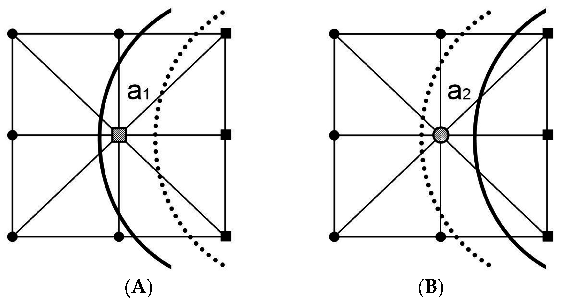
3.3. The Improved Schemes by Caiazzo, Chen, Hu, et al.

In recent years, a few schemes were proposed to improve the accuracy and Galilean invariance of the momentum exchange method. Caiazzo and Junk [48] presented an modified momentum exchange method according to the asymptotic expansion technique,

$$F_i(x_b)=e_i{\tilde{f}}_i(x_f,t)-e_{\overline{i}}{\tilde{f}}_{\overline{i}}(x_s,t)-2{\mathsf{\omega }}_i{e}_i-{\mathsf{\omega }}_i{c}_s^{-2}\text{(}{c}_s^{-2}{\left|e_i\cdot u_b\right|}^{\text{2}}-u_b^2)e_i$$

(22)

Clausen and Aidun [49] obtained a similar correction to reduce the error of normal stress and investigated the effect on the rheological properties in particle suspensions. Lorrenz et al. [50] investigated Galilean invariance and accuracy of the improved method by simulating particle suspensions with Lees-Edwards boundary conditions [51] and a shear flow test.

For a particle suspension model without fluid inside, simulations by Wen et al. [20] and Chen et al. [22] showed when the impulse force was not included, the numerical results of the conventional exchange equation deviated from both results of finite element method and LBM with the stress integration method, no matter the curved boundary condition or the halfway bounce-back boundary condition was used. Because the conventional momentum exchange equation, namely Equation (16), for stationary boundaries was verified to be accurate [37] and the impulse force was not necessary for LBM with the stress integration method, Chen et al. [22] thought that the problem could lie in the calculation of momentum exchange in the moving boundary treatment.

Considering a distribution function as a mass component, the distribution function will gain an additional momentum when it collides with a moving boundary. Due to the constant discrete velocities in LBM, the additional part has to be modified by adjusting the particle distribution function in the bounce back procedure like the last part of Equation (17). The modification leads to a net mass transfer on a fluid-solid link through the physical boundary for the direct simulation of suspending particles without interior fluid. From another angle, the net mass transfer can be seen as a bit of fluid mass which is covered (or uncovered) and is injected, at the time step, back to (or down from) the fluid field [22], as shown in Figure 3. The initial momenta of the net fluid mass must be complemented to CME and a straightforward correct is given by Chen et al. [22]:

$$F_i(x_b)=e_i{\tilde{f}}_i(x_f,t)-e_{\overline{i}}{\tilde{f}}_{\overline{i}}(x_s,t)-\frac{2{\mathsf{\omega }}_i\mathsf{\rho }}{c_s^2}\text{(}{e}_i\cdot u_b\text{)}{u}_b$$

(23)

Associating with the Aidun’s method [12,20], the total impulse produced from Equations (18) and (19) is equal to the total initial momenta of the fluid which is covered or uncovered by the unit length boundary when the boundary shifts from a lattice node to its neighbor.

Figure 3. A schematic illustration of a moving boundary on lattice grid. (Chen et al., 2013 [22]).

Figure 3. A schematic illustration of a moving boundary on lattice grid. (Chen et al., 2013 [22]).

Based on the finite-volume lattice Boltzmann method, Hu et al. [52] proposed a modified momentum exchange method to compute the interactions between fluid and particle. Their aim is to remove the common restriction in the momentum exchange method, in which the boundary points are set at the middle of the grid lines or the intersection of the solid boundaries and the grid lines. The particulate surface is described by some arc (area) elements, and the inside fluid is also used. Considering the control volume, the momentum exchange method is modified by

$$F_i(x_b)=2e_i\left[{\tilde{f}}_{\overline{i}}(x_s,t)-\frac{{\mathsf{\omega }}_i\mathsf{\rho }}{c_s^2}\text{(}{e}_i\cdot u_b\text{)}\right]V_{\overline{i}}$$

(24)

where $V_{\overline{i}}$ is the area (volume) of the local curved edge. By means of numerical integration, the fluid mass which collide with an arc (area) element in the control volume is obtained.

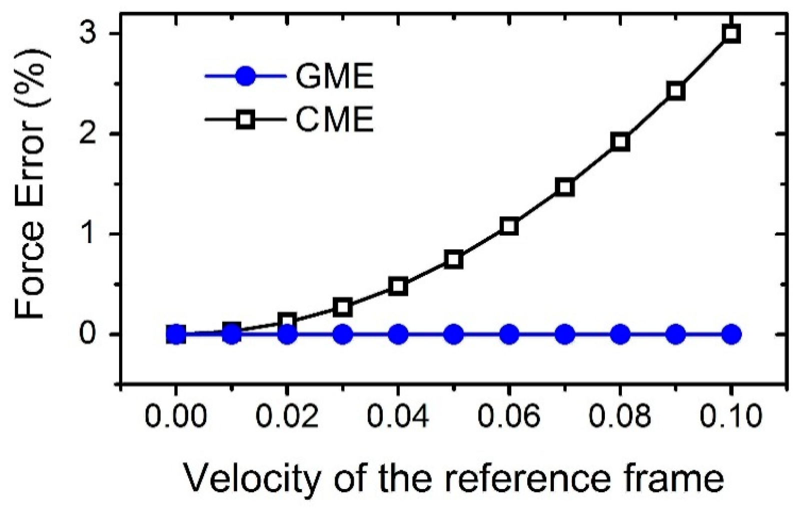
3.4. The Galilean Invariant Hydrodynamics Force by Wen et al.

The interfacial momentum transfer can be generalized by a common schematic diagram as shown in Figure 4, in which a moving boundary is located between a fluid node $x_f$ and a boundary node $x_s$ and the boundary has a velocity $v$ at the point of intersection $b$. In the collision step, the distribution function ${\tilde{f}}_{\overline{i}}(x_b\text{,}t)$ has to be calculated by the half-way bounce-back boundary condition [10,12] or the curved boundary conditions [20,22,37,53], in which the forcing terms [54,55,56] must be included based on the boundary velocity.

Figure 4. A common schematic diagram to illustrate a moving boundary crossing a fluid-solid link at the point of intersection b. x_f and x_s denote the adjacent fluid and solid nodes. The boundary has a velocity v at the point b. (Wen et al., 2014 [13]).

Figure 4. A common schematic diagram to illustrate a moving boundary crossing a fluid-solid link at the point of intersection b. x_f and x_s denote the adjacent fluid and solid nodes. The boundary has a velocity v at the point b. (Wen et al., 2014 [13]).

Galilean invariance is a fundamental physical property; however, although the dynamics of lattice Boltzmann equation in hydrodynamic restrict meets Galilean invariance [57], this property needs a specific consideration in the treatment of the fluid-structure interactions. According to the theorem of momentum, the momentum transfer through a moving boundary is correlated to the relative velocity and then is independent of the speed of reference frame. Crossing the point of intersection $b$, the mass component ${\tilde{f}}_i(x_f\text{,}t)$ has the velocity $(e_i-v)$ relative to the boundary and contributes a momentum increment $(e_i-v){\tilde{f}}_i(x_f\text{,}t)$ to the boundary. Simultaneously, the mass component ${\tilde{f}}_{\overline{i}}(x_s\text{,}t)$ has the relative velocity $(e_{\overline{i}}-v)$ and decreases a momentum $(e_{\overline{i}}-v){\tilde{f}}_{\overline{i}}(x_s\text{,}t)$ from the boundary. Thus, the Galilean invariant momentum exchange method (GME) can be defined by

$$F_i(x_b)=(e_i-v){\tilde{f}}_i(x_f\text{,}t)-(e_{\overline{i}}-v){\tilde{f}}_{\overline{i}}(x_s\text{,}t)$$

(25)

It is clear that GME turns into CME when the boundary is motionless. GME evaluates the hydrodynamic force in the fluid-structure interaction and works on the motion state of a moving boundary, but has not any direct influence on distribution functions. The similar relative velocity was mentioned in the study of Krithivasan et al. [58].

A simple theoretical analysis is employed to compare GME and CME. Suppose the system in Figure 4 is relative static and is physically related to a reference frame with arbitrary uniform velocity $-v$. It is equivalent to an equilibrium system in which the fluid and boundary have the same uniform velocity $v$. Substituting Equation (4) into Equation (16), the hydrodynamic force on a fluid-solid link can be evaluated:

$$\begin{array}{c}{F}_i=e_i{f}_i^{(eq)}(x_f\text{,}t)-e_{\overline{i}}{f}_{\overline{i}}^{(eq)}(x_s\text{,}t)\\ =e_i\mathsf{\rho }{\mathsf{\omega }}_i[1+3(e_i\cdot v)+\frac{9}{2}{(e_i\cdot v)}^2-\frac{3}{2}{v}^2]-e_{\overline{i}}\mathsf{\rho }{\mathsf{\omega }}_{\overline{i}}[1+3(e_{\overline{i}}\cdot v)+\frac{9}{2}{(e_{\overline{i}}\cdot v)}^2-\frac{3}{2}{v}^2]\\ =2\mathsf{\rho }{\mathsf{\omega }}_i{e}_i+3\mathsf{\rho }{\mathsf{\omega }}_i[3{(e_i\cdot v)}^2-v^2]e_i\text{.}\end{array}$$

(26)

Because of the term $3\mathsf{\rho }{\mathsf{\omega }}_i[3{(e_i\cdot v)}^2-v^2]e_i$, the hydrodynamic force is abnormally connected to the speed of the reference frame, and thus the conventional equation presents an inherent flaw of Galilean invariance.

As the discrete velocity $e_i$ is constant, Galilean invariance cannot be satisfied on a single fluid-solid link, just like a single $e_i$ cannot express the fluid velocity of a lattice node. However, since the discrete velocity set is symmetrical, the Galilean invariant force evaluation can be achieved locally on the lattice. Without loss of generality, the boundary is assumed to intersect with the discrete velocities, $e_1$, $e_5$ and $e_8$. Substituting Equation (4) into Equation (25) and summating the three directions, the local hydrodynamic force can be analyzed

$$\begin{array}{l}F=F_1+F_5+F_8\\ ={\displaystyle \sum _{i=1,5,8}[(e_i-v)f_i^{(eq)}(x_f\text{,}t)-(e_{\overline{i}}-v)f_{\overline{i}}^{(eq)}(x_s\text{,}t)]}\\ ={\displaystyle \sum _{i=1,5,8}\{2\mathsf{\rho }{\mathsf{\omega }}_i{e}_i+3\mathsf{\rho }{\mathsf{\omega }}_i[3{(e_i\cdot v)}^2-v^2]e_i-6\mathsf{\rho }{\mathsf{\omega }}_i(e_i\cdot v)v\}}\\ ={\displaystyle \sum _{i=1,5,8}2\mathsf{\rho }{\mathsf{\omega }}_i{e}_i}.\end{array}$$

(27)

The local hydrodynamic force remains constant regardless of the reference speed, therefore GME is proven to be completely Galilean invariant in the equilibrium system.

Another simple simulation can quantitatively show the difference between GME and CME. A vertical thin plate is placed in the relatively static fluid without boundary. GME and CME are used to compute the one-sided pressure of the plate and the equilibrium system is connected to a reference frame. The percentage of the computational errors by GME and CME are shown in Figure 5. It is clear that CME violates Galilean invariance whereas GME fully satisfies in the equilibrium system. The case is independent of the relaxation time and the plate’s length.

Figure 5. Relative errors in the one-sided pressure on a vertical thin plate in the relatively stationary fluid without boundaries. This equilibrium system is connected to various velocities of the reference frame. Since it properly considers the boundary velocity, Galilean invariant momentum exchange method (GME) is the Galilean invariant and thus has a very high computational accuracy. (Wen et al., 2014 [13]).

Figure 5. Relative errors in the one-sided pressure on a vertical thin plate in the relatively stationary fluid without boundaries. This equilibrium system is connected to various velocities of the reference frame. Since it properly considers the boundary velocity, Galilean invariant momentum exchange method (GME) is the Galilean invariant and thus has a very high computational accuracy. (Wen et al., 2014 [13]).

GME is further examined in a dynamic fluid field in which a cylinder sedimentates in a vertical channel. The width of the channel is 0.4 cm and the cylinder diameter is 0.1 cm. The fluid and particle densities are 1 g/cm³ and 1.03 g/cm³, and the kinematic viscosity is 0.01 cm²/s. The cylinder is located at 0.076 cm to the left channel wall, and then it moves under the gravity acceleration |G| = 980 cm²/s. The width of the channel is 120 lattice units and the length is 10 times the width. The simulations apply the second-order interpolation boundary condition [56] on the single-relaxation-time model with the relaxation time $\mathsf{\tau }=0.6$. The particle mass is 8.0896 × 10⁻³ g and the inertia moment is 1.0112 × 10⁻⁵ g∙cm². The Reynolds numbers is defined by $Re=d{u}_p/v$, where d is the channel width, u_p is the final velocity of the particle and $v$ is the kinematic viscosity. The highly consistent results are obtained by using the multireflection boundary condition [59] on the multiple-relaxation-time model with the diagonal relaxation matrix $S=\text{diag}(0\text{, 1.64, 1.54, 0, 1.9, 0, 1.9,}1/\mathsf{\tau }\text{,}1/\mathsf{\tau })$ [23,30].

Figure 6a,b draws the compare with the simulating results from the momentum exchange methods by Aidun et al. (ALD) [12] and the lattice-type-dependent momentum exchange method (LME) [20], together with the benchmarks calculated by the arbitrary Lagrangian–Eulerian technique (ALE) [60,61]. The hydrodynamic forces computed by GME extremely agree with the benchmarks, while the results by ALD and LME have large fluctuations. Please note that all of the data from GME are raw, whereas the data from ALD and LME have been smoothed by using the adjacent-averaging method per 30 points for the horizontal forces and per 100 points for the vertical forces. As so much improvement in the force evaluation is achieved, the force fluctuation of GME is very small and the time average becomes unnecessary.

Figure 6. (a) Time-dependent horizontal forces and (b) time-dependent vertical forces evaluated by GME, lattice-type-dependent momentum exchange method (LME), and Aidun’s method (ALD), compared with the ALE benchmark. The density of the cylinder is 1.03 g/cm³. The GME data is raw, whereas the ALD and LME data have been smoothed by the adjacent-averaging method. (Wen et al., 2014 [13]).

Figure 6. (a) Time-dependent horizontal forces and (b) time-dependent vertical forces evaluated by GME, lattice-type-dependent momentum exchange method (LME), and Aidun’s method (ALD), compared with the ALE benchmark. The density of the cylinder is 1.03 g/cm³. The GME data is raw, whereas the ALD and LME data have been smoothed by the adjacent-averaging method. (Wen et al., 2014 [13]).

Figure 7a,b draws the accuracy of the velocity and angle velocity computed by GME, ALD and LME. All velocities from GME are very smooth and in excellent agreement with the ALE benchmarks, whereas the results from ALD and LME clearly fluctuate with some deviations. The GME results are so accurate and steady that the time average of the velocities is totally unnecessary.

Figure 7. Time-dependent (a) horizontal velocities and (b) angular velocities evaluated by GME, LME, and ALD, compared with the ALE benchmark. (Wen et al., 2014 [13]).

Figure 7. Time-dependent (a) horizontal velocities and (b) angular velocities evaluated by GME, LME, and ALD, compared with the ALE benchmark. (Wen et al., 2014 [13]).

The deviations of forces and velocities are quantitatively analyzed by a relative L₂-norm error, which is defined by

$$E=\frac{{\{\int {[f(t)-F(t)]}^{2}dt\}}^{\raisebox{1ex}{$1$}\!\left/ \!\raisebox{-1ex}{$2$}\right.}}{{\{\int {[F(t)]}^{2}dt\}}^{\raisebox{1ex}{$1$}\!\left/ \!\raisebox{-1ex}{$2$}\right.}}$$

(28)

To investigate the effects of lattice scale, the lattice width of the channel increases gradually from 50 to 200 lattice units, while the length remains 10 times the width. For Equation (28), f(t) is a LBM result and F(t) is an ALE result. Figure 8a illustrates that the relative errors of the GME results rapidly decrease with the increase of the lattice scale. However, the relative errors of the ALD and LME results always remain very high and are more than one order larger than those from GME. To investigate the influences of Reynolds number, we perform a set of simulations in which the particle densities increase from 1.02 to 1.22 g/cm³, and the corresponding Reynolds number grows gradually from 6.13 to 34.75. As shown in Figure 8b, the relative L₂-norm errors reflect the fluctuation range in particle velocities. Here, f(t) is the simulation result and F(t) is the smoothed simulation result by the adjacent-averaging method per 20 points. It is clear that the GME results are more accurate and far steadier than the ALD and LME results. Peng et al. [62] confirmed the computational accuracy and Galilean invariance of GME by theoretical analyses and numerical simulations.

Figure 8. (a) The relative L₂-norm error of the horizontal forces (Fx, black) and vertical forces (Fy, blue) with increasing lattice scales; (b) The relative L₂-norm errors of the horizontal velocity (Vx, black) and the angular velocity (ω, red) with various Reynolds numbers. (Wen et al., 2014 [13]).

Figure 8. (a) The relative L₂-norm error of the horizontal forces (Fx, black) and vertical forces (Fy, blue) with increasing lattice scales; (b) The relative L₂-norm errors of the horizontal velocity (Vx, black) and the angular velocity (ω, red) with various Reynolds numbers. (Wen et al., 2014 [13]).

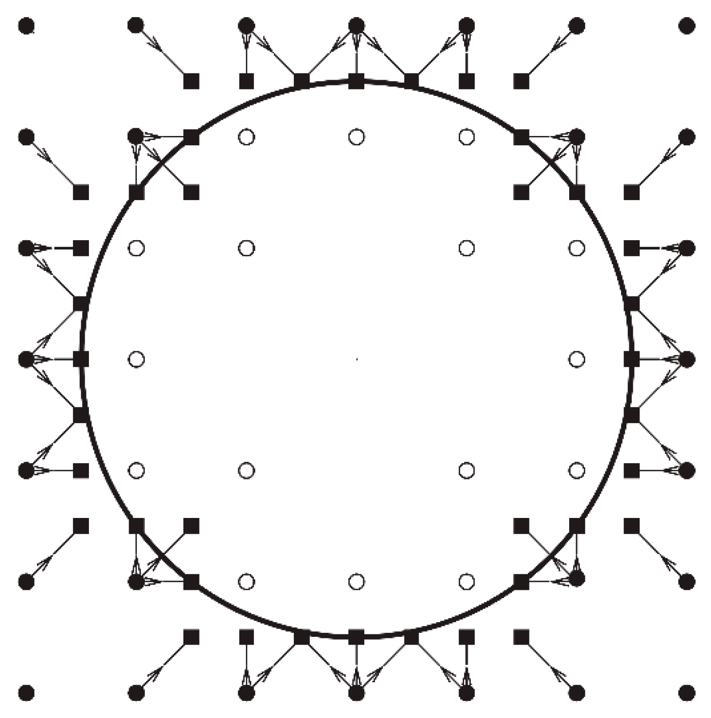
4. Refill of New Fluid Nodes

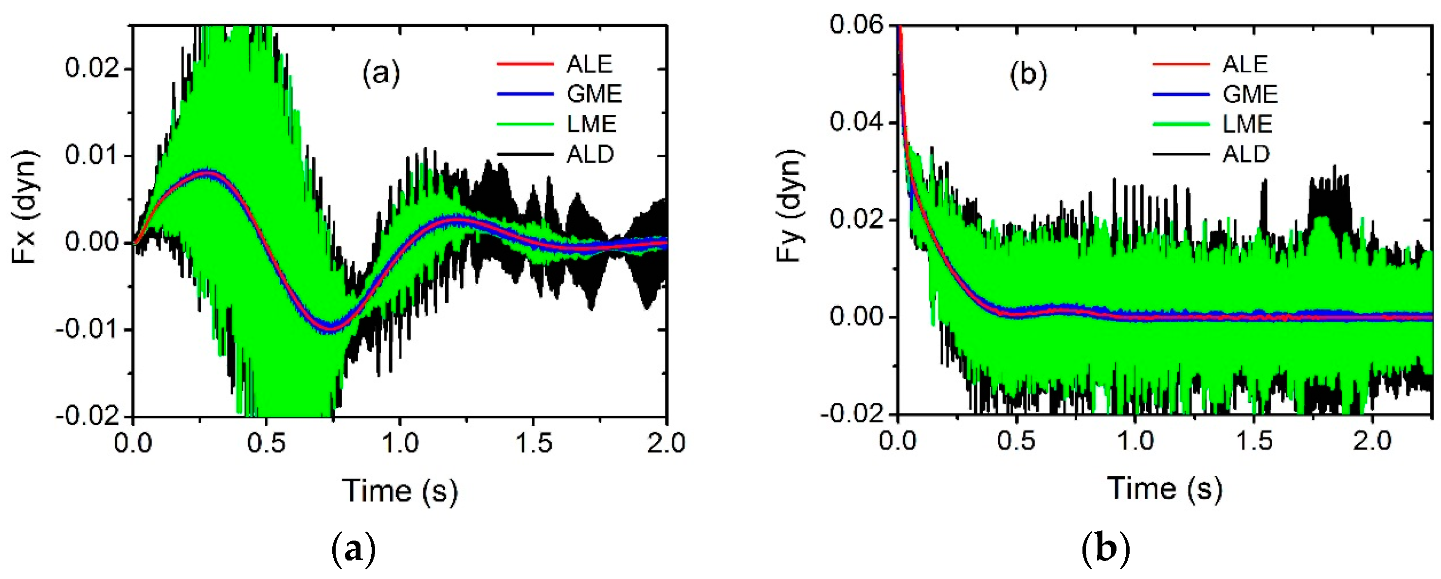
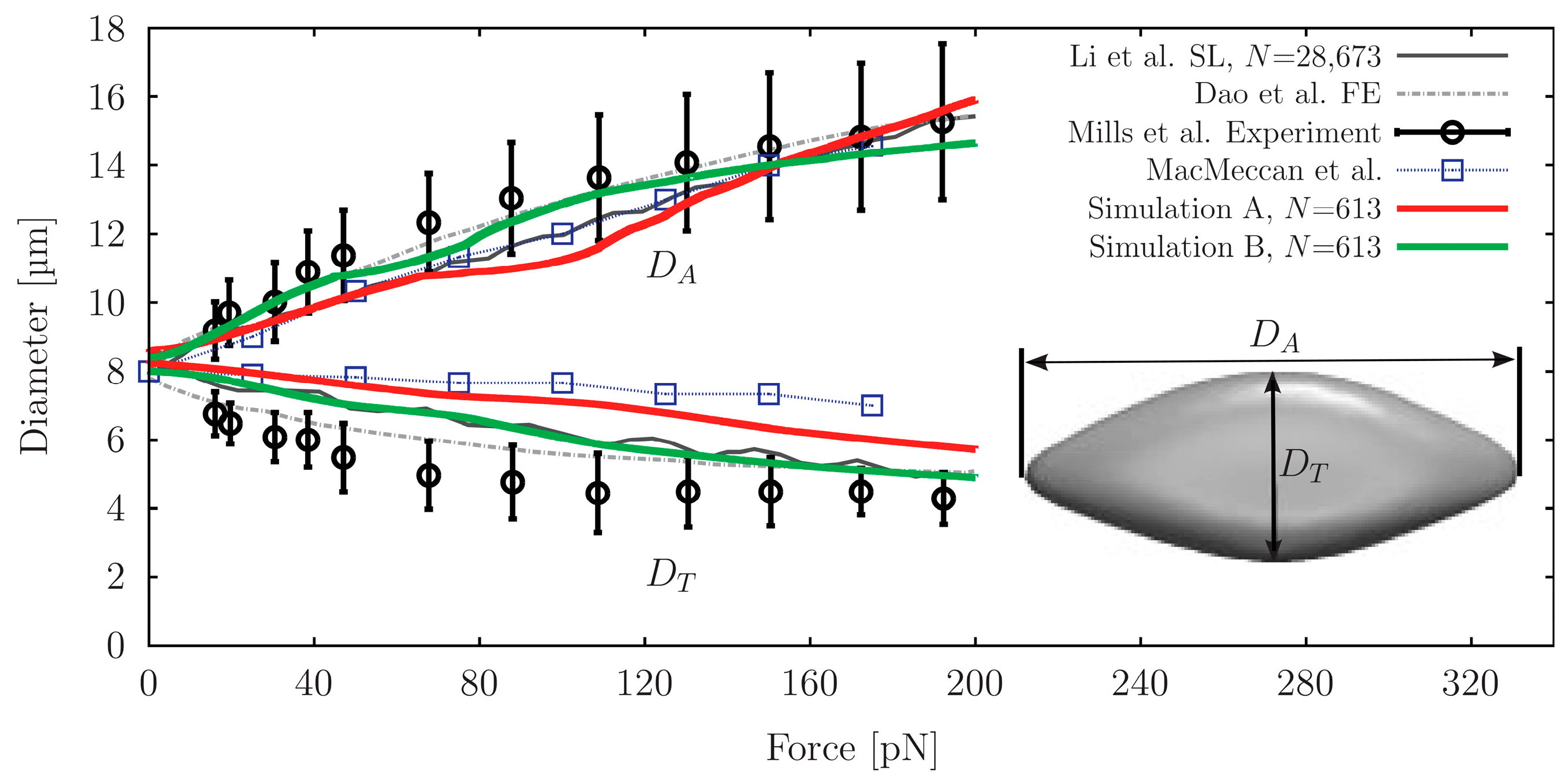
While a suspended particle is moving in fluid some lattices will be covered and uncovered by the particle, and then the type of these lattices will be changed consequently. Ladd’s method does not need a further process because all lattice nodes, both inside and outside of a particle, are treated as fluid nodes. When an interior node changes into an exterior node, it is justified if the density of the interior node approximates the right characteristic of the exterior one. This may be only true in the situations that the particulate acceleration is low. If a particle is accelerated, the fluid directly behind the particle typically suffers a lower pressure while the adjacent inner node bears a rather high pressure [50]. This may reduce the stability of the particle velocity update. For the methods without inner fluid node, when a lattice node is changing from a particle node to a fluid one, its properties has to be refilled, such as density, velocity and distribution functions [13,20,22]. Here, we introduce some algorithms used in practice as follows.

Aidun et al. [12] presented a simple algorithm to refill the newborn fluid node when they directly simulated particle suspensions. When a boundary node is uncovered due to the movement of the solid particle and becomes a new fluid node, its density is obtained with the following relation:

$$\mathsf{\rho }(x\text{,}t)=\frac{1}{N}{\displaystyle \sum _N\mathsf{\rho }(x+e_i\text{,}t)}$$

(29)

where $x$ is the newborn fluid lattice node and $N$ indicates the number of fluid nodes adjacent to this lattice node. The equation shows that the fluid density of the newborn node is equal to the average density of its neighboring lattice nodes. The velocity of the solid boundary node at the same time step is used as the macroscopic velocity of the new fluid node,

$$u(x\text{,}t)=U(t)+\Omega (t)\times (x-R(t))$$

(30)

where $U$ is the particle translational velocity, $\Omega$ is the angular velocity and $R$ is the particulate mass center. The distribution functions on the newly uncovered node are set as the equilibrium distribution functions calculated by the density and velocity above.

Lallemand and Luo [56] used a second-order normal extrapolation to calculate the missed distribution functions. Along the direction of a chosen discrete velocity $e_i$, the extrapolation considers the boundary normal direction to maximize the quantity $\widehat{n}\cdot e_i$, where $\widehat{n}$ is the normal vector out of the wall. For instance, the unknown distribution functions $\{f_i(x)\}$ at node $x$ as drawn in Figure 9 can be calculated by the extrapolation formula as follow:

$$f_i(x)=3f_i(x^{\prime })-3f_i(x^{″})+f_i(x^{‴})$$

(31)

where $x^{‴}$ is the next lattice node along the direction $x^{\prime }$ to $x^{″}$.

Figure 9. A boundary is moving with velocity u_w. The circles (○) and disks (●) denote fluid and boundary nodes, respectively. The squares (□) denote the nodes turning from boundary nodes to fluid ones at a time step. The solid and dotted curves are the positions of wall boundary at time t and t + 1, respectively. (Lallemand and Luo, 2003 [56]).

Figure 9. A boundary is moving with velocity u_w. The circles (○) and disks (●) denote fluid and boundary nodes, respectively. The squares (□) denote the nodes turning from boundary nodes to fluid ones at a time step. The solid and dotted curves are the positions of wall boundary at time t and t + 1, respectively. (Lallemand and Luo, 2003 [56]).

Caiazzo [63] suggested a refill scheme by reconstructing the equilibrium and non-equilibrium parts separately according to an asymptotic analysis prediction. The initialization of the populations includes an approximation of the non-equilibrium part which, in practice, can be copied simply from a neighbor of the new fluid node. The equilibrium part is computed basing on the density and velocity which can be gotten by a simple first order extrapolation.

$$f_i(x,t)=f_i^{eq}(x,t,\mathsf{\rho },u)+f_i^{neq}(x+e_j,t)\text{}$$

(32)

where $e_j$ indicates the extrapolation direction according to the boundary velocity at a point of interface close to the new fluid node. Lorenz et al. [50,51] employed a similar approach, in which the equilibrium part was calculated basing on the local pressure.

Krithivasan et al. [58] recently developed a diffuse bounce-back boundary condition to simulate moving boundaries instead of imposing the no-slip conditions. This scheme ensures positive-definite populations and retains the simplicity of bounce-back technique. Meanwhile it suggests a refill algorithm to model distributions at the fluid nodes uncovered due to solid movement by quasi-equilibrium distributions. The scheme is demonstrated to reduce force fluctuations and diminish the requirements of interpolation or extrapolation. However, a diffuse boundary condition will introduce some degree of boundary slip [64,65,66], which would damage simulating accuracy and Galilean invariance.

Fang et al. [13,67] used the fluid nodes around the newborn fluid nodes to extrapolate the distribution functions of the newborn fluid nodes. If the extrapolating participants are more than one, the newborn distribution functions are assigned as their average. Three extrapolation algorithms, namely neighbor-node average (A1), linear extrapolation (A2) and second order extrapolation (A3), are as follows [13]

$$\text{A1}:f_i(x)=\frac{1}{N}{\displaystyle \sum _N{f}_i(x^{\prime })}$$

(33)

$$\text{A2}:f_i(x)=\frac{1}{N}{\displaystyle \sum _{N}2f_i(x^{\prime })-f_i(x^{″})}$$

(34)

$$\text{A3}:f_i(x)=\frac{1}{N}{\displaystyle \sum _{N}3f_i(x^{\prime })-3f_i(x^{″})+f_i(x^{‴})}$$

(35)

where $N$ is the number of extrapolation participants. The density and velocity of the newborn fluid node at the present time step are computed by the resulting distribution functions,

$$\mathsf{\rho }(x,t)={\displaystyle \sum _i{f}_i(x)}$$

(36)

$$u(x,t)=\frac{1}{\mathsf{\rho }(x,t)}{\displaystyle \sum _i{e}_i{f}_i(x)}$$

(37)

They investigated the three algorithms in the simulations of cylinder sedimentation as shown in Figure 10. It is evident that the algorithm with second order extrapolation can remarkably reduce the fluctuations.

Peng et al. [62] proposed a refill scheme by velocity-constrained normal extrapolation based on the multiple-relaxation-time LBM. After the missing distribution functions of a newborn fluid node are completed by the normal extrapolation refill scheme, all moments at the newborn node are computed by multiplying the transfer matrix $\text{M}$,

$$\mathbf{m}\text{(}x\text{,}t\text{)}=\text{M}\cdot \widehat{\mathbf{f}}\text{(}x\text{,}t\text{)}$$

(38)

where $\widehat{\mathbf{f}}$ indicates the temporary distribution functions. Then the momentum moments are constrained to use the velocity of the nearest boundary,

$$J={\mathsf{\rho }}_0{u}_b$$

(39)

This makes a new moment vector ${\mathbf{m}}^{*}\text{(}x\text{,}t\text{)}$. Finally, transfer ${\mathbf{m}}^{*}\text{(}x\text{,}t\text{)}$ back to the distribution functions as

$$\mathbf{f}\text{(}x\text{,}t\text{)}={\text{M}}^{\text{-1}}\cdot {\mathbf{m}}^{*}\text{(}x\text{,}t\text{)}$$

(40)

They found that this constraint could significantly reduce the fluctuations in the hydrodynamic forces.

Figure 10. The horizontal forces in cylinder sedimentation. GME is coupled with the different algorithms to fill newborn fluid nodes, neighbor-node average (A1), linear extrapolation (A2) and second-order extrapolation (A3). (Wen et al., 2014 [13]).

Figure 10. The horizontal forces in cylinder sedimentation. GME is coupled with the different algorithms to fill newborn fluid nodes, neighbor-node average (A1), linear extrapolation (A2) and second-order extrapolation (A3). (Wen et al., 2014 [13]).

Obviously, the scheme is not unique to compute the unknown values, such as density, velocities and distribution functions, on the lattice nodes which move from non-fluid to fluid region. In the particle sedimentation in low Reynolds number, these schemes will produce similar macroscopic results. However, at the micro-scale, they lead to different fluctuating ranges in hydrodynamic forces, which inevitably influence the accuracy and stability of simulations.

5. Applications

As a method to evaluate hydrodynamic force, the momentum exchange method possesses the advantages of simplicity, efficiency, accuracy and robustness. Remarkably, it is independent of the boundary geometry, preventing from solving the Navier–Stokes equations in complex boundary geometries in the boundary-integral methods [10]. Since the pioneer works of Ladd [10,11] and Aidun [12,36], the lattice Boltzmann method has developed into a popular tool for simulations of particle suspensions. In this section, we review some representative applications, such as movements of rigid particles, interactions of deformation particles, particle suspensions in turbulent flow and multiphase flow, etc. Particle Brownian motion due to thermal fluctuations and particle surface charges are not covered.

5.1. Rigid Particle Movements

The sedimentation of a single rigid particle is a common case in the simulations of particle suspensions [68,69,70,71] and is often used as a benchmark [13,20,22]. Qi [72] simulated sedimentations of spherical and non-spherical particles in finite-Reynolds-number flows and observed phenomena of drafting, kissing and tumbling motion of two particles in a smooth-walled channel. Recently, Wen et al. [13] used circle sedimentations to verify Galilean invariance of the momentum exchange method. The configuration is the same to that in Section 3.4. The simulation system is related to several uniform frames of reference in order to investigate Galilean invariance of the hydrodynamic force [13]. Explicitly, the additional uniform velocities V = 0, 0.01, 0.02 are initially assigned to the fluid, the particle and the channel.

Figure 11 presents the time-dependent trajectories, angular velocities, horizontal velocities and vertical velocities relative to the channel, comparing with the results by CME and ALE [60,61]. Obviously, regardless of the reference speeds, the GME results are always in excellent agreement with the ALE benchmarks. This supports that GME is highly accurate and Galilean invariant in dynamic fluid. Oppositely, even if the reference frame is motionless, the CME results show noticeable deviations from the benchmark. And the differences become larger and larger when the reference speed increases. These suggest that CME is non-Galilean invariant and is not suitable for moving boundaries.

The lateral migration of a particle suspended in a Poiseuille flow is a classic case. A suspending biconcave particle in a tube flow is studied by using the multiple-relaxation-time lattice Boltzmann method together with GME. The biconcave shape of a red blood cell (RBC) follows the descriptive equation proposed by Fung et al. in 1980s [73] and the characteristic radius is 15 lattice units.

The biconcave particles are located at 0.04 and 0.02 cm away from the low channel wall and at the center of the channel in the horizontal direction. Figure 12 draws the particle trajectories at Reynolds numbers 12 and 3, respectively. The biconcave particle shows lateral migrating movement and equilibrium state, which are close to the classic Segré–Silberberg effect [46,47]. Because of the interaction of the parabolic velocity distribution of Poiseuille flow and the biconcave shape, the particulate movement exhibits regular waves and nonuniform rotation. Remarkably, they observe two lateral equilibrium positions corresponding to the particulate releasing positions [74]. The biconcave particle is in successive postures in a rotating period and Figure 13 illustrates a set of velocity contours to draw the dynamic flow field.

Figure 11. Time-dependent (a) trajectories; (b) angular velocities; (c) horizontal velocities; and (d) vertical velocities relative to the channel. The density of the cylinder is 1.03 g/cm³ and the terminal Reynolds number is 8.33. The dynamic simulation system is connected to three velocities of the reference frame, i.e., V = 0, 0.01, and 0.02. (Wen et al., 2014 [13]).

Figure 11. Time-dependent (a) trajectories; (b) angular velocities; (c) horizontal velocities; and (d) vertical velocities relative to the channel. The density of the cylinder is 1.03 g/cm³ and the terminal Reynolds number is 8.33. The dynamic simulation system is connected to three velocities of the reference frame, i.e., V = 0, 0.01, and 0.02. (Wen et al., 2014 [13]).

Figure 12. The trajectories of a suspending biconcave particle migrating in a Poiseuille flow. The Reynolds numbers are (a) Re = 3 and (b) Re = 12. The biconcave particles are located at 0.04 and 0.02 cm away from the low channel wall. The classic Segré–Silberberg effect with a circular particle is represented by the black trajectories. (Wen et al., 2013 [74]).

Figure 12. The trajectories of a suspending biconcave particle migrating in a Poiseuille flow. The Reynolds numbers are (a) Re = 3 and (b) Re = 12. The biconcave particles are located at 0.04 and 0.02 cm away from the low channel wall. The classic Segré–Silberberg effect with a circular particle is represented by the black trajectories. (Wen et al., 2013 [74]).

Figure 13. The velocity contours of the fluid around the biconcave particles. (a)–(f) represent six different postures in a half rotation period. (Wen et al., 2013 [74]).

Figure 13. The velocity contours of the fluid around the biconcave particles. (a)–(f) represent six different postures in a half rotation period. (Wen et al., 2013 [74]).

GME can be easily implemented in 3D simulations. The Segré–Silberberg effect [46,47] is repeated by simulating a neutrally buoyant rigid sphere migrating laterally in a tube Poiseuille flow. Figure 14 draws two trajectories of the spheres, which are released at the dimensionless radial positions of r*/R = 0.66 and 0.21, where r* is the radial distance from the tube centerline. The numerical results are highly consistent with the experiments by Karnis et al. [47]. This verifies that GME is competent to 3D simulations of particle suspensions.

Chen et al. [22] simulated an elliptical particle sedimentating in a vertical channel in order to verified their improved momentum exchange method. The major axis is 0.05 cm and the minor axis is 0.025 cm. The kinematic viscosity of the fluid is 1 × 10⁻⁶ m²/s. The channel width is 0.4 cm and is 104 lattice units in the numerical simulation. The density ratio of the solid particle and fluid is 1.1. Figure 15 shows an elliptical sedimentation with a moderate Reynolds number 6.6. It is clear that the results of the three improved schemes agree very well with the benchmarks of the finite element method.

Figure 14. Three-dimensional simulations of the Segré–Silberberg effect by the lattice Boltzmann equation with GME. (Wen et al., 2014 [13]).

Figure 14. Three-dimensional simulations of the Segré–Silberberg effect by the lattice Boltzmann equation with GME. (Wen et al., 2014 [13]).

Figure 15. The trajectories and orientations of the particle with Reynolds number 6.6 obtained by the finite element method [75] and LBM with the curved boundary condition. The results of the three improved schemes [12,20,22,48] are in good agreement with the benchmark. (Chen et al., 2013 [22]).

Figure 15. The trajectories and orientations of the particle with Reynolds number 6.6 obtained by the finite element method [75] and LBM with the curved boundary condition. The results of the three improved schemes [12,20,22,48] are in good agreement with the benchmark. (Chen et al., 2013 [22]).

To determinate the critical parameters in platelet margination, Reasor et al. [76] investigated the margination dependences on hematocrit, platelet shape, and viscosity ratio of plasma to cytoplasm. The hydrodynamic force is evaluated by the momentum exchange method. Their results emphasize that an increase in hematocrit increases the rate of margination. The viscosity ratio between the interior cytoplasm and suspending fluid can considerably alter the rate of margination. Spherical particles tend to migrate more quickly than disks. The effect of platelet aspect ratio is demonstrated in Figure 16. The spherical-shaped particles have a diameter of 1.73 μm. The platelet-shaped particles are oblate spheroids and rigid, with a major diameter of 2.3 μm and a thickness of 1.0 μm. The disk-shaped particles with a major diameter of 3.26 μm and a thickness of 0.523 μm. It can be seen that both the mean distance to the wall and the standard deviation are reduced with decreasing aspect ratio. The peak concentrations at the wall are larger for the spherical particles and the distributions evolve more rapidly than the disk-shaped particles. The simulations also show the lateral migration of particles with various shapes in tube flow.

Figure 16. Temporal evolution of platelet distributions for the concentration 0.2 for (a) spheres; (b) platelets; and (c) disk shaped particles. The initial and ending end views of the tube are also given to display the distribution of platelets before and after margination. (Reasor et al., 2013 [76]).

Figure 16. Temporal evolution of platelet distributions for the concentration 0.2 for (a) spheres; (b) platelets; and (c) disk shaped particles. The initial and ending end views of the tube are also given to display the distribution of platelets before and after margination. (Reasor et al., 2013 [76]).

5.2. Deformation Particle Interactions

A growing interest in the simulations of deformation suspensions has promoted the development of coupled methods, in which LBM is combined with an appropriate boundary model to capture the particle deformations. Aidun et al. implemented a spectrin-link red blood cell membrane method coupled with the lattice Boltzmann method [7,76,77,78,79]. In the method, the particle is represented by a triangular shell mesh, on which the local hydrodynamic force is calculated by momentum exchange method.

To capture the deformation process, Reasor et al. [77,78] took a spherical capsule to create a baseline RBC mesh whose surface includes a network of 613 points. Then, 59% of its initial volume was deflated while the surface area keeps constant. The RBC radius was 12 lattice units which approximately equates to 4 μm. Figure 17 illustrates the continuous deformation from a sphere to a biconcave RBC. The equilibrium biconcave shape was reached after 25,000 time steps and is an artifact of minimizing the Helmholtz free energy which involves contributions due to bending.

The spectrin-link method is further compared with experiments [80] and other computational approaches [81] by an optical tweezer experiment performed by Mills et al. [80]. The RBC is initially static and is immersed in fluid which simulates blood plasma and hemoglobin. The axial and transverse diameters of an RBC are stretched by optical tweezers with silica beads attached at both ends. As shown in Figure 18, the simulating results are in good agreement with previous researches. MacMeccan et al. [77] simulated multiply deformable particle suspensions by coupling the lattice Boltzmann method with finite element analysis. They studied more than 200 fluid-filled and initially spherical capsules in unbounded shear flow. The capsules occupied 40% volume fraction and had identical properties with RBC membranes. Aidun and Clausen [7] further investigated the deformation and interaction of more than 2000 deformable particle suspensions. Melchionna et al. [82,83] simulated cardiovascular blood flow, aiming to cardiovascular diagnosis for commodity clinical applications.

Figure 17. A spherical particle is deflated and become biconcave particle of red blood cell. (a) t = 0; (b) t = 5000; (c) t = 10000; (d) t = 15000; (e) t = 20000; (f) t = 25000. (Reasor et al., 2012 [78]).

Figure 17. A spherical particle is deflated and become biconcave particle of red blood cell. (a) t = 0; (b) t = 5000; (c) t = 10000; (d) t = 15000; (e) t = 20000; (f) t = 25000. (Reasor et al., 2012 [78]).

Figure 18. The axial and transverse diameters, D_A and D_T, in μm of the RBC plotted against the applied force. The simulating results are compared to the high-resolution spectrin-level modeling [81], the high-resolution the finite element method [84], the experiments [80], and using the LB–FE implementation [77]. (Reasor et al., 2012 [78]).

Figure 18. The axial and transverse diameters, D_A and D_T, in μm of the RBC plotted against the applied force. The simulating results are compared to the high-resolution spectrin-level modeling [81], the high-resolution the finite element method [84], the experiments [80], and using the LB–FE implementation [77]. (Reasor et al., 2012 [78]).

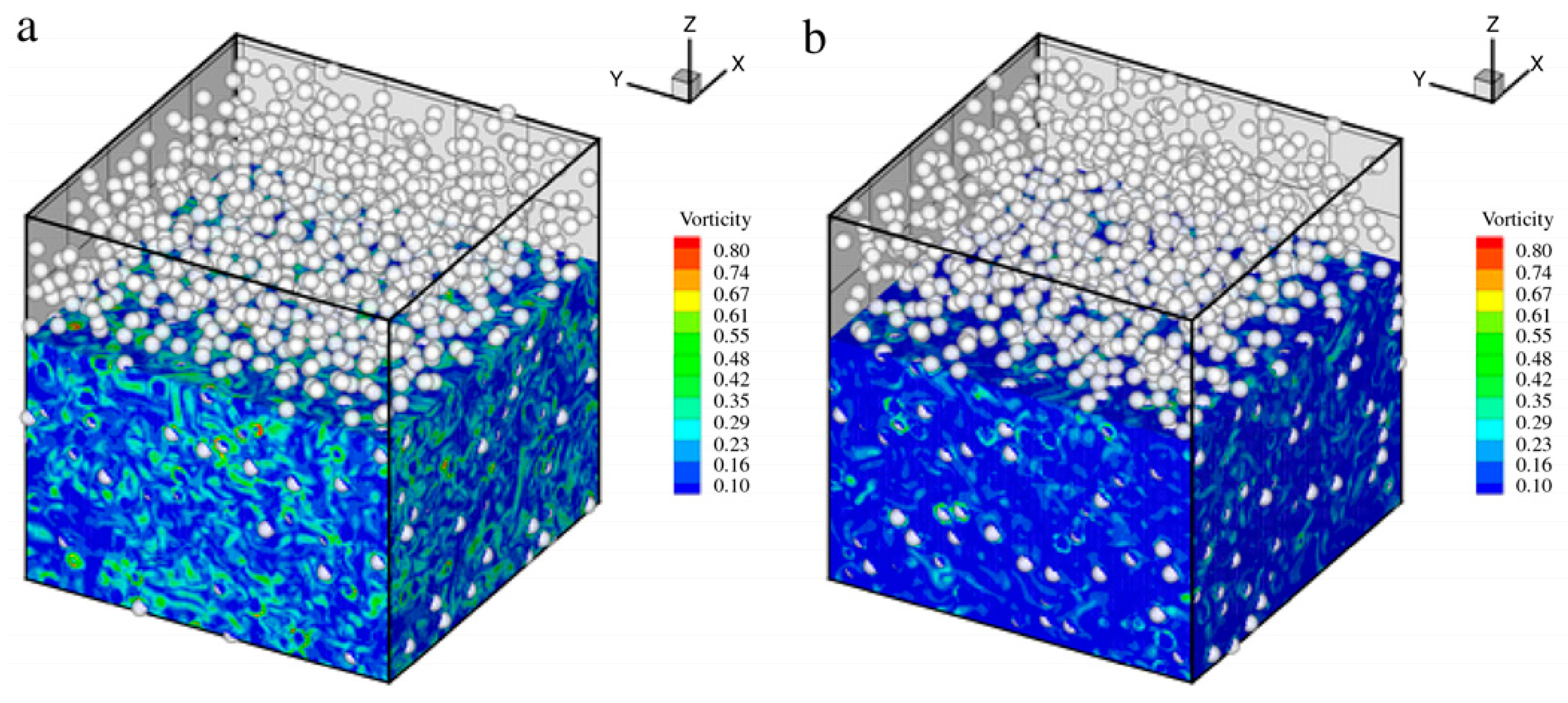
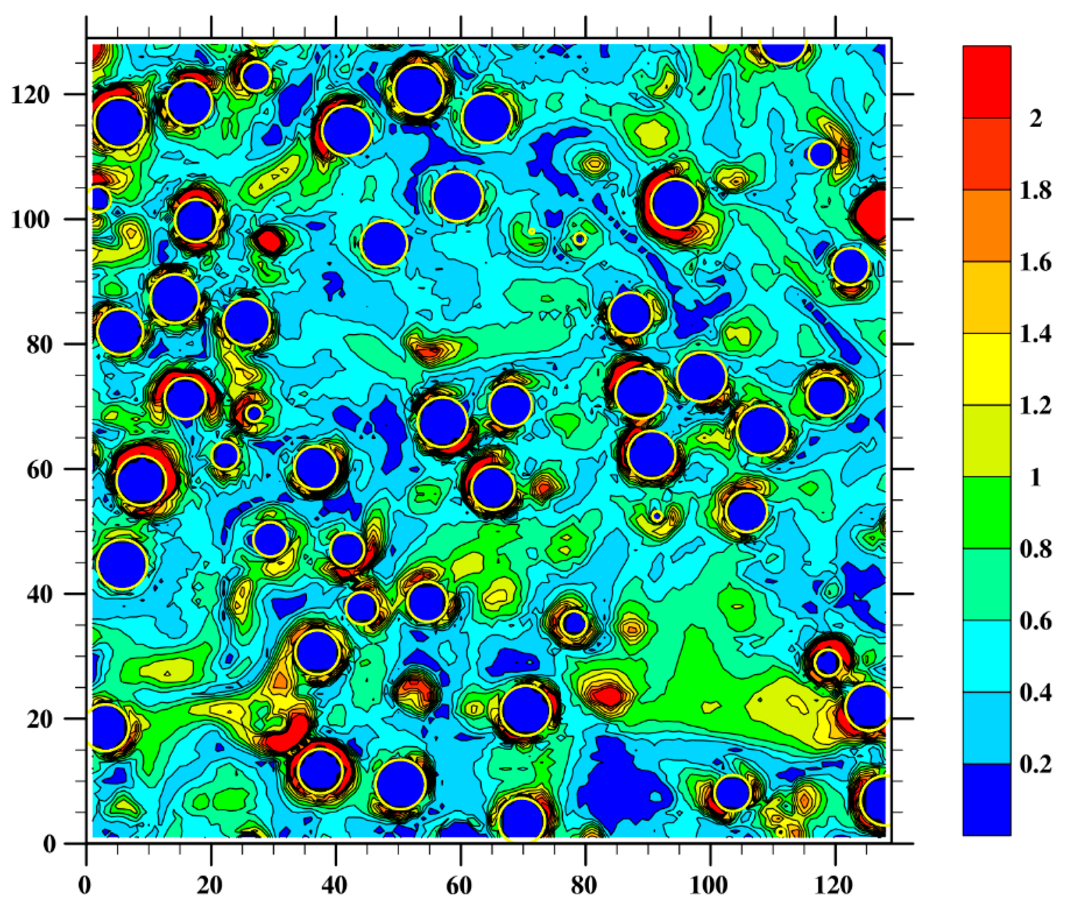
5.3. Particle Suspensions in Turbulent Flow

Turbulent flows laden with gas bubbles, small droplets or solid particles are relevant to a wide variety of engineering applications and natural processes, such as plankton dynamics, dust storms, pollutant transport [85]. Using the lattice Boltmzann method coupled with the momentum exchange method, Wang et al. [85,86,87] made a comparative analysis to single-phase turbulence and particle-laden turbulence and studied a decaying isotropic turbulence laden with finite-size particles of Kolmogorov to Taylor microscale sizes. Zhang et al. [88,89] investigated the differential settling of cohesive sediment and the non-equilibrium flocculation of cohesive sediments in homogeneous turbulent flows.

For the particle-laden turbulence simulations, Gao et al. [85] randomly released particles into the fluid domain after the single-phase flow field developed till a converged velocity-derivative skewness. They implemented a second-order interpolation boundary condition [56] and MPI parallel acceleration based on multiple-relaxation-time LBM. A short-range repulsive force is indroduced to prevent particles from voerlap. Figure 19 draws the vorticity contours of the two evolution times, 1.27 Te and 2.12 Te, where Te is the eddy turnover time. The compuational domain is 256³ and contains 2304 rigid particles with uniform diameter 11 lattice units. The density ratio of particle and fluid is 2.56. A top layer of fluid has been removed in order to show the scatter of a portion of the particles. It is clear that the magnitude of vorticity diminishes with the time evolution.

Figure 19. Vorticity contour at (a) 1.27 Te and (b) 2.12 Te. A layer of fluid is removed to show the particles in the top portion. (Gao et al., 2013 [85]).

Figure 19. Vorticity contour at (a) 1.27 Te and (b) 2.12 Te. A layer of fluid is removed to show the particles in the top portion. (Gao et al., 2013 [85]).

The two-dimensional visualizations of the vorticity magnitude and the particle scatter are provided by horizontally cutting the fluid through the slice near the center of the domain [86,87]. The compuational domain is 256³ and contains 6400 rigid particles with uniform diameter 8 lattice units. The density ratio of particle and fluid is 5. The Reynolds number of particles are about 10. The turbulent flow is driven by the well-known stochastic forcing scheme of Eswaran and Pope [90]. The particles are observed often associating with high voritcity values (the red spots), as shown in Figure 20. This suggests that, in turbulent flow, motions of finite size particles can produce small-scale flow structures near their surfaces.

Figure 20. Horizontal snapshots of vorticity contour and particle location in particle-laden turbulent channel flow. The presence of particles can be observed often associating with high vorticity values (represented by the colors towards the red end). This indicates relatively larger dissipation near particle surfaces. (Wang et al., 2014 [86]).

Figure 20. Horizontal snapshots of vorticity contour and particle location in particle-laden turbulent channel flow. The presence of particles can be observed often associating with high vorticity values (represented by the colors towards the red end). This indicates relatively larger dissipation near particle surfaces. (Wang et al., 2014 [86]).

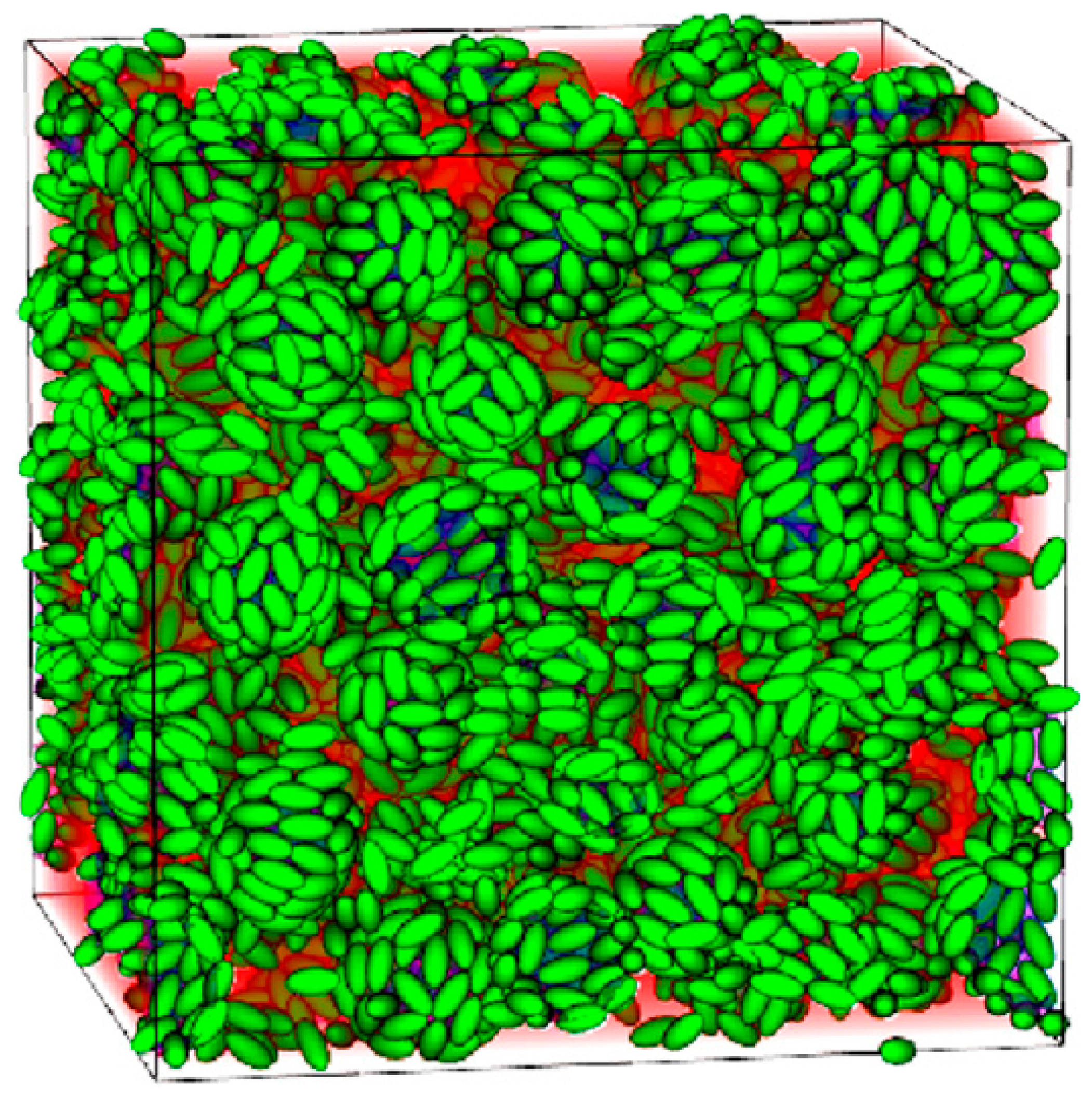
5.4. Particle Suspensions in Multiphase Flow

Particles or colloids suspended in multiphase flow are commonly encountered in scientific researches and engineering applications such as particle self-assembly, emulsion stabilized by particles and microbe transport in air-water flow. Joshi and Sun [91] combined the Shan-Chen multiphase flow model [9,92,93,94,95] with particle suspension to study the capillary interactions between two suspended particles, which were on a liquid-vapor interface and suffered different external forces. The pseudopotential model is applied to calculate the nonideal force in multiphase flow and the momentum exchange method is employed to evaluate the fluid-particle interactions, coupling with the lubrication and Hookean force between pairs of particles. The computational domain uses a 300² lattice with periodic boundaries. 36 suspended particles of radius 4.8 lattice units are arrayed in the multiphase flow. The liquid-vapor density ratio is about 30 and the relaxation time is 1. Figure 21 exhibits particle movements during a phase transition process. The adhesive force in the multiphase system is −0.04 and is corresponding to a 77° equilibrium contact angle. Therefore, the particles are hydrophilic. With the development of the two phases, particles are inclined to stay at the gas-liquid interface and then obstruct the phases from growing.

The combined model is further extended to a three-dimensional droplet simulations, considering drop evaporation and particle deposition [96,97]. Adjusting the substrate surface wettability, namely the surface energy, the substrate patterning can control the particle deposition. The computational domain is 250 × 250 × 100 in lattice unit for investigating the surface wetting effect on drop dynamics. In the pattern, the central band is 70 lattice units in width and is hydrophilic, while the side bands are relatively hydrophobic. The equilibrium contact angle of the central hydrophilic band is 30°, and those of the side bands are 60°, 90°, and 120°, respectively. The liquid drop includes 90 particles (10% by volume). Due to an initial offset, the drop impacts the substrate outside the central band. Figure 22 shows that repelling from the bands with relatively low energy, the initially offset drop with suspending particles gradually and automatically moves into the hydrophilic central band. The moving velocities of the drops are affected both by the effective viscosity of the drop and the relative wetting strengths of the bands. Similarly, Liang et al. [98] simulated the self-assemblies of colloidal particles on the substrate and investigated the lateral capillary forces and many-body effects.

Figure 21. Spinodal decomposition with suspended particles simulated by LBM. The particles are initially arranged in a uniform array. The particles tend to inhibit coarsening of the interface and accumulate at the liquid-vapor interface, as the green liquid domains begin to coalesce and form. (Joshi et al., 2009 [91]).

Figure 21. Spinodal decomposition with suspended particles simulated by LBM. The particles are initially arranged in a uniform array. The particles tend to inhibit coarsening of the interface and accumulate at the liquid-vapor interface, as the green liquid domains begin to coalesce and form. (Joshi et al., 2009 [91]).

Figure 22. Effect of surface wetting strength on drop dynamics for a liquid drop containing suspending particles. The hydrophilic bands (red) keep 30° contact angle, while the hydrophobic bands are (a) 60°, (b) 90°, and (c) 120° contact angle. The faster driving velocity can be clearly seen in the case (c). (Joshi et al., 2010 [96]).

Figure 22. Effect of surface wetting strength on drop dynamics for a liquid drop containing suspending particles. The hydrophilic bands (red) keep 30° contact angle, while the hydrophobic bands are (a) 60°, (b) 90°, and (c) 120° contact angle. The faster driving velocity can be clearly seen in the case (c). (Joshi et al., 2010 [96]).

Particle stabilized emulsions are ubiquitous in the food and cosmetics industry. Jansen and Hurting [99] simulated interactions of multiple spheroidal particles in a multiphase flow lattice Boltzmann method. They demonstrated that the transition from a Bijel to a Pickering emulsion is dependent of the particle concentration, the contact angle, and the ratio of the solvents. Günther et al. [100] investigated anisotropic particles at liquid interfaces by simulating emulsions stabilized by particles with complex shapes. The computational domain is a cubic volume with a side length 256 lattice units and periodic boundary conditions are applied. The particles are ellipsoids with major axis 12 and minor axis 6 lattice units and occupy a volume concentration of 0.2. The particle surface has equilibrium contact angles of 90°. As shown in Figure 23 in which the ratio of two phase fluids is 5:2, the ellipsoid particles assemble to some clusters surrounding a fluid phase in an other phase and become Pickering emulsions. They also simulated the Bijel in which the ratio of two phase fluids is 1:1.

Figure 23. A snapshot of Pickering emulsions stabilized by ellipsoidal particles with an aspect ratio 2 and a volume concentration 0.2. (Günther et al., 2013 [100]).

Figure 23. A snapshot of Pickering emulsions stabilized by ellipsoidal particles with an aspect ratio 2 and a volume concentration 0.2. (Günther et al., 2013 [100]).

6. Conclusions

The momentum exchange method is a native scheme in the lattice Boltzmann method. It directly uses discrete velocity and distribution function to evaluate hydrodynamic force. This is totally different from the stress integration method and the immersed boundary method, which have to compute the stress tensor before force evaluation. Therefore, the momentum exchange method has a gift to obtain the simplest and most accurate hydrodynamic force in LBM. Since hydrodynamic force is evaluated based on the momentum transfer on each fluid-solid link, the momentum exchange method only needs local data and is independent of boundary geometry. This endues it with excellent computational efficiency and parallel performance.

Thus far, the momentum exchange method has promoted LBM to become a popular tool for numerical simulations of fluid-structure interactions. Its computational accuracy and Galilean invariance on stationary and moving boundaries in moderate Reynolds numbers have been verified [13,37]. In practice, all kinds of simulations of fluid-structure interactions can benefit from the efficient method. An open issue is to further investigate its computation accuracy in more complex circumstances, such as high Reynolds number flow even turbulence, slip boundary, multiphase flow and so on.

References

1. Higuera, F.J.; Succi, S.; Benzi, R. Lattice gas dynamics with enhanced collisions. Europhys. Lett. 1989, 9, 345–349. [Google Scholar] [CrossRef]
2. Qian, Y.H.; d’Humières, D.; Lallemand, P. Lattice BGK models for Navier–Stokes equation. Europhys. Lett. 1992, 17, 479–484. [Google Scholar] [CrossRef]
3. Chen, S.Y.; Chen, H.D.; Martinez, D.; Matthaeus, W. Lattice boltzmann model for simulation of magnetohydrodynamics. Phys. Rev. Lett. 1991, 67, 3776–3779. [Google Scholar] [CrossRef] [PubMed]
4. Chen, H.D.; Chen, S.Y.; Matthaeus, W.H. Recovery of the Navier–Stokes equations using a lattice-gas Boltzmann method. Phys. Rev. A 1992, 45, R5339–R5342. [Google Scholar] [CrossRef] [PubMed]
5. Benzi, R.; Succi, S.; Vergassola, M. The lattice Boltzmann equation: Theory and applications. Phys. Rep. 1992, 222, 145–197. [Google Scholar] [CrossRef]
6. Chen, S.; Doolen, G.D. Lattice Boltzmann method for fluid flows. Annu. Rev. Fluid Mech. 1998, 30, 329–364. [Google Scholar] [CrossRef]
7. Aidun, C.K.; Clausen, J.R. Lattice-Boltzmann method for complex flows. Annu. Rev. Fluid Mech. 2010, 42, 439–472. [Google Scholar] [CrossRef]
8. Dünweg, B.; Ladd, A.J.C. Lattice Boltzmann Simulations of Soft Matter Systems. In Advanced Computer Simulation Approaches for Soft Matter Sciences III; Springer: Berlin/Heidelberg, Germany, 2009; pp. 89–166. [Google Scholar]
9. Chen, L.; Kang, Q.; Mu, Y.; He, Y.-L.; Tao, W.-Q. A critical review of the pseudopotential multiphase lattice Boltzmann model: Methods and applications. Int. J. Heat Mass Transf. 2014, 76, 210–236. [Google Scholar] [CrossRef]
10. Ladd, A.J.C. Numerical simulations of particulate suspensions via a discretized Boltzmann equation. Part 1. Theoretical foundation. J. Fluid Mech. 1994, 271, 285–309. [Google Scholar] [CrossRef]
11. Ladd, A.J.C. Numerical simulations of particulate suspensions via a discretized Boltzmann equation. Part 2. Numerical results. J. Fluid Mech. 1994, 271, 311–339. [Google Scholar] [CrossRef]
12. Aidun, C.K.; Lu, Y.N.; Ding, E.-J. Direct analysis of particulate suspensions with inertia using the discrete Boltzmann equation. J. Fluid Mech. 1998, 373, 287–311. [Google Scholar] [CrossRef]
13. Wen, B.; Zhang, C.; Tu, Y.; Wang, C.; Fang, H. Galilean invariant fluid–solid interfacial dynamics in lattice Boltzmann simulations. J. Comput. Phys. 2014, 266, 161–170. [Google Scholar] [CrossRef]
14. He, X.; Doolen, G. Lattice Boltzmann method on curvilinear coordinates system: Flow around a circular cylinder. J. Comput. Phys. 1997, 134, 306–315. [Google Scholar] [CrossRef]
15. Inamuro, T.; Maeba, K.; Ogino, F. Flow between parallel walls containing the lines of neutrally buoyant circular cylinders. Int. J. Multiph. Flow 2000, 26, 1981–2004. [Google Scholar] [CrossRef]
16. Li, H.; Lu, X.; Fang, H.; Qian, Y. Force evaluations in lattice Boltzmann simulations with moving boundaries in two dimensions. Phys. Rev. E 2004, 70, 026701. [Google Scholar] [CrossRef] [PubMed]
17. Peskin, C.S. Numerical analysis of blood flow in the heart. J. Comput. Phys. 1977, 25, 220–252. [Google Scholar] [CrossRef]
18. Feng, Z.-G.; Michaelides, E.E. The immersed boundary-lattice Boltzmann method for solving fluid–particles interaction problems. J. Comput. Phys. 2004, 195, 602–628. [Google Scholar] [CrossRef]
19. Zhou, Q.; Fan, L.-S. A second-order accurate immersed boundary-lattice Boltzmann method for particle-laden flows. J. Comput. Phys. 2014, 268, 269–301. [Google Scholar] [CrossRef]
20. Wen, B.; Li, H.; Zhang, C.; Fang, H. Lattice-type-dependent momentum-exchange method for moving boundaries. Phys. Rev. E 2012, 85, 016704. [Google Scholar] [CrossRef] [PubMed]
21. Caiazzo, A.; Junk, M.; Rheinländer, M. Comparison of analysis techniques for the lattice Boltzmann method. Comput. Math. Appl. 2009, 58, 883–897. [Google Scholar] [CrossRef]
22. Chen, Y.; Cai, Q.; Xia, Z.; Wang, M.; Chen, S. Momentum-exchange method in lattice Boltzmann simulations of particle-fluid interactions. Phys. Rev. E 2013, 88, 013303. [Google Scholar] [CrossRef] [PubMed]
23. Lallemand, P.; Luo, L.-S. Theory of the lattice Boltzmann method: Dispersion, dissipation, isotropy, Galilean invariance, and stability. Phys. Rev. E 2000, 61, 6546–6562. [Google Scholar] [CrossRef]
24. D’Humières, D.; Ginzburg, I.; Krafczyk, M.; Lallemand, P.; Luo, L.-S. Multiple-relaxation-time lattice Boltzmann models in three dimensions. Philos. Trans. R. Soc. Lond. A 2002, 360, 437–451. [Google Scholar] [CrossRef] [PubMed]
25. Ginzburg, I.; Verhaeghe, F.; d’Humières, D. Two-relaxation-time lattice Boltzmann scheme: About parametrization, velocity, pressure and mixed boundary conditions. Commun. Comput. Phys. 2008, 3, 427–478. [Google Scholar]
26. Karlin, I.V.; Ferrante, A.; Öttinger, H.C. Perfect entropy functions of the lattice Boltzmann method. Europhys. Lett. 1999, 47, 182–188. [Google Scholar] [CrossRef]
27. Succi, S.; Karlin, I.V.; Chen, H. Colloquium: Role of the H theorem in lattice Boltzmann hydrodynamic simulations. Rev. Mod. Phys. 2002, 74, 1203–1220. [Google Scholar] [CrossRef]
28. D’Humières, D. Generalized lattice-Boltzmann equations. Rarefied Gas Dyn. 1994, 159, 450–458. [Google Scholar]
29. Luo, L.-S. Theory of the lattice Boltzmann method: Lattice Boltzmann models for nonideal gases. Phys. Rev. E 2000, 62, 4982–4996. [Google Scholar] [CrossRef]
30. Luo, L.-S.; Liao, W.; Chen, X.; Peng, Y.; Zhang, W. Numerics of the lattice Boltzmann method: Effects of collision models on the lattice Boltzmann simulations. Phys. Rev. E 2011, 83, 056710. [Google Scholar] [CrossRef] [PubMed]
31. Ladd, A.J.C.; Verberg, R. Lattice-Boltzmann simulations of particle-fluid suspensions. J. Stat. Phys. 2001, 104, 1191–1251. [Google Scholar] [CrossRef]
32. Nguyen, N.-Q.; Ladd, A.J.C. Lubrication corrections for lattice-Boltzmann simulations of particle suspensions. Phys. Rev. E 2002, 66, 046708. [Google Scholar] [CrossRef] [PubMed]
33. Nguyen, N.-Q.; Ladd, A.J.C. Sedimentation of hard-sphere suspensions at low Reynolds number. J. Fluid Mech. 2005, 525, 73–104. [Google Scholar] [CrossRef]
34. Başağaoğlu, H.; Meakin, P.; Succi, S.; Redden, G.R.; Ginn, T.R. Two-dimensional lattice Boltzmann simulation of colloid migration in rough-walled narrow flow channels. Phys. Rev. E 2008, 77, 031405. [Google Scholar] [CrossRef] [PubMed]
35. Başağaoğlu, H.; Allwein, S.; Succi, S.; Dixon, H.; Carrola, J.T., Jr.; Stothoff, S. Two-and three-dimensional lattice Boltzmann simulations of particle migration in microchannels. Microfluid. Nanofluid. 2013, 15, 785–796. [Google Scholar] [CrossRef]
36. Aidun, C.K.; Lu, Y. Lattice Boltzmann simulation of solid particles suspended in fluid. J. Stat. Phys. 1995, 81, 49–61. [Google Scholar] [CrossRef]
37. Mei, R.; Yu, D.; Shyy, W.; Luo, L.-S. Force evaluation in the lattice Boltzmann method involving curved geometry. Phys. Rev. E 2002, 65, 041203. [Google Scholar] [CrossRef] [PubMed]
38. Filippova, O.; Hänel, D. Grid refinement for lattice-BGK models. J. Comput. Phys. 1998, 147, 219–228. [Google Scholar] [CrossRef]
39. Mei, R.; Luo, L.-S.; Shyy, W. An accurate curved boundary treatment in the lattice Boltzmann method. J. Comput. Phys. 1999, 155, 307–330. [Google Scholar] [CrossRef]
40. Mei, R.; Shyy, W.; Yu, D.; Luo, L.-S. Lattice Boltzmann method for 3-D flows with curved boundary. J. Comput. Phys. 2000, 161, 680–699. [Google Scholar] [CrossRef]
41. Ding, E.-J.; Aidun, C.K. Extension of the lattice-Boltzmann method for direct simulation of suspended particles near contact. J. Stat. Phys. 2003, 112, 685–708. [Google Scholar] [CrossRef]
42. Bouzidi, M.; Firdaouss, M.; Lallemand, P. Momentum transfer of a Boltzmann-lattice fluid with boundaries. Phys. Fluids 2001, 13, 3452–3459. [Google Scholar] [CrossRef]
43. Guo, Z.L.; Zheng, C.G.; Shi, B.C. An extrapolation method for boundary conditions in lattice Boltzmann method. Phys. Fluids 2002, 14, 2007–2010. [Google Scholar] [CrossRef]
44. Kao, P.-H.; Yang, R.-J. An investigation into curved and moving boundary treatments in the lattice Boltzmann method. J. Comput. Phys. 2008, 227, 5671–5690. [Google Scholar] [CrossRef]
45. Bao, J.; Yuan, P.; Schaefer, L. A mass conserving boundary condition for the lattice Boltzmann equation method. J. Comput. Phys. 2008, 227, 8472–8487. [Google Scholar] [CrossRef]
46. Segré, G.; Silberberg, A. Radial particle displacements in poiseuille flow of suspensions. Nature 1961, 189, 209–210. [Google Scholar] [CrossRef]
47. Karnis, A.; Goldsmith, H.L.; Mason, S.G. The flow of suspensions through tubes: V. inertial effects. Can. J. Chem. Eng. 1966, 44, 181–193. [Google Scholar] [CrossRef]
48. Caiazzo, A.; Junk, M. Boundary forces in lattice Boltzmann: Analysis of momentum exchange algorithm. Comput. Math. Appl. 2008, 55, 1415–1423. [Google Scholar] [CrossRef]
49. Clausen, J.R.; Aidun, C.K. Galilean invariance in the lattice-Boltzmann method and its effect on the calculation of rheological properties in suspensions. Int. J. Multiph. Flow 2009, 35, 307–311. [Google Scholar] [CrossRef]
50. Lorenz, E.; Caiazzo, A.; Hoekstra, A.G. Corrected momentum exchange method for lattice Boltzmann simulations of suspension flow. Phys. Rev. E 2009, 79, 036705. [Google Scholar] [CrossRef] [PubMed]
51. Lorenz, E.; Hoekstra, A.G.; Caiazzo, A. Lees-edwards boundary conditions for lattice Boltzmann suspension simulations. Phys. Rev. E 2009, 79, 036706. [Google Scholar] [CrossRef] [PubMed]
52. Hu, Y.; Li, D.; Shu, S.; Niu, X. Modified momentum exchange method for fluid-particle interactions in the lattice Boltzmann method. Phys. Rev. E 2015, 91, 033301. [Google Scholar] [CrossRef] [PubMed]
53. Huang, H.; Yang, X.; Krafczyk, M.; Lu, X.-Y. Rotation of spheroidal particles in couette flows. J. Fluid Mech. 2012, 692, 369–394. [Google Scholar] [CrossRef]
54. Luo, L.-S. Unified theory of lattice Boltzmann models for nonideal gases. Phys. Rev. Lett. 1998, 81, 1618–1621. [Google Scholar] [CrossRef]
55. Guo, Z.; Zheng, C.; Shi, B. Discrete lattice effects on the forcing term in the lattice Boltzmann method. Phys. Rev. E 2002, 65, 046308. [Google Scholar] [CrossRef] [PubMed]
56. Lallemand, P.; Luo, L.-S. Lattice Boltzmann method for moving boundaries. J. Comput. Phys. 2003, 184, 406–421. [Google Scholar] [CrossRef]
57. Qian, Y.-H.; Zhou, Y. Complete Galilean-invariant lattice BGK models for the Navier–Stokes equation. Europhys. Lett. 1998, 42, 359–364. [Google Scholar] [CrossRef]
58. Krithivasan, S.; Wahal, S.; Ansumali, S. Diffused bounce-back condition and refill algorithm for the lattice Boltzmann method. Phys. Rev. E 2014, 89, 033313. [Google Scholar] [CrossRef] [PubMed]
59. Ginzburg, I.; d’Humières, D. Multireflection boundary conditions for lattice Boltzmann models. Phys. Rev. E 2003, 68, 066614. [Google Scholar] [CrossRef] [PubMed]
60. Hu, H.H.; Joseph, D.D.; Crochet, M.J. Direct simulation of fluid particle motions. Theor. Comput. Fluid Dyn. 1992, 3, 285–306. [Google Scholar] [CrossRef]
61. Hu, H.H.; Patankar, N.A.; Zhu, M.Y. Direct Numerical Simulations of Fluid–Solid Systems Using the Arbitrary Lagrangian–Eulerian Technique. J. Comput. Phys. 2001, 169, 427–462. [Google Scholar] [CrossRef]
62. Peng, C.; Teng, Y.; Hwang, B.; Guo, Z.; Wang, L.-P. Implementation issues and benchmarking of lattice Boltzmann method for moving rigid particle simulations in a viscous flow. Comput. Math. Appl. 2015, in press. [Google Scholar] [CrossRef]
63. Caiazzo, A. Analysis of lattice Boltzmann nodes initialisation in moving boundary problems. Prog. Comput. Fluid Dyn. 2008, 8, 3–10. [Google Scholar] [CrossRef]
64. Ansumali, S.; Karlin, I.V. Kinetic boundary conditions in the lattice Boltzmann method. Phys. Rev. E 2002, 66, 026311. [Google Scholar] [CrossRef] [PubMed]
65. Tang, G.H.; Tao, W.Q.; He, Y.L. Lattice Boltzmann method for gaseous microflows using kinetic theory boundary conditions. Phys. Fluids 2005, 17, 058101. [Google Scholar] [CrossRef]
66. Guo, Z.L.; Shi, B.; Zhao, T.S.; Zheng, C. Discrete effects on boundary conditions for the lattice Boltzmann equation in simulating microscale gas flows. Phys. Rev. E 2007, 76, 056704. [Google Scholar] [CrossRef] [PubMed]
67. Fang, H.; Wang, Z.; Lin, Z.; Liu, M. Lattice Boltzmann method for simulating the viscous flow in large distensible blood vessels. Phys. Rev. E 2002, 65, 051925. [Google Scholar] [CrossRef] [PubMed]
68. Wan, R.-Z.; Fang, H.-P.; Lin, Z.; Chen, S. Lattice Boltzmann simulation of a single charged particle in a Newtonian fluid. Phys. Rev. E 2003, 68, 011401. [Google Scholar] [CrossRef] [PubMed]
69. Li, H.; Fang, H.; Lin, Z.; Xu, S.X.; Chen, S. Lattice Boltzmann simulation on particle suspensions in a two-dimensional symmetric stenotic artery. Phys. Rev. E 2004, 69, 031919. [Google Scholar] [CrossRef] [PubMed]
70. Zhang, C.-Y.; Shi, J.; Tan, H.-L.; Liu, M.-R.; Kong, L.-J. Sedimentation of a single charged elliptic cylinder in a Newtonian fluid by lattice Boltzmann method. Chin. Phys. Lett. 2004, 21, 1108–1110. [Google Scholar]
71. Zhang, C.-Y.; Tan, H.-L.; Liu, M.-R.; Kong, L.-J.; Shi, J. Lattice Boltzmann simulation of sedimentation of a single charged elastic dumbbell in a Newtonian fluid. Chin. Phys. Lett. 2005, 22, 896–899. [Google Scholar]
72. Qi, D. Lattice-Boltzmann simulations of particles in non-zero-Reynolds-number flows. J. Fluid Mech. 1999, 385, 41–62. [Google Scholar] [CrossRef]
73. Fung, Y.C. Biomechanics; Springer: New York, NY, USA, 1981. [Google Scholar]
74. Wen, B.-H.; Chen, Y.-Y.; Zhang, R.-L.; Zhang, C.-Y.; Fang, H.-P. Lateral migration and nonuniform rotation of biconcave particle suspended in Poiseuille flow. Chin. Phys. Lett. 2013, 30, 064701. [Google Scholar] [CrossRef]
75. Xia, Z.; Connington, K.W.; Rapaka, S.; Yue, P.; Feng, J.J.; Chen, S. Flow patterns in the sedimentation of an elliptical particle. J. Fluid Mech. 2009, 625, 249–272. [Google Scholar] [CrossRef]
76. Reasor, D.A.; Mehrabadi, M.; Ku, D.N.; Aidun, C.K. Determination of critical parameters in platelet margination. Ann. Biomed. Eng. 2013, 41, 238–249. [Google Scholar] [CrossRef] [PubMed]
77. MacMeccan, R.M.; Clausen, J.R.; Neitzel, G.P.; Aidun, C.K. Simulating deformable particle suspensions using a coupled lattice-Boltzmann and finite-element method. J. Fluid Mech. 2009, 618, 13–39. [Google Scholar] [CrossRef]
78. Reasor, D.A., Jr.; Clausen, J.R.; Aidun, C.K. Coupling the lattice-Boltzmann and spectrin-link methods for the direct numerical simulation of cellular blood flow. Int. J. Numer. Meth. Fluids 2012, 68, 767–781. [Google Scholar] [CrossRef]
79. Wu, J.; Aidun, C.K. Simulating 3D deformable particle suspensions using lattice Boltzmann method with discrete external boundary force. Int. J. Numer. Meth. Fluids 2010, 62, 765–783. [Google Scholar] [CrossRef]
80. Mills, J.P.; Qie, L.; Dao, M.; Lim, C.T.; Suresh, S. Nonlinear elastic and viscoelastic deformation of the human red blood cell with optical tweezers. Mech. Chem. Biosys. 2004, 1, 169–180. [Google Scholar]
81. Li, J.; Dao, M.; Lim, C.; Suresh, S. Spectrin-level modeling of the cytoskeleton and optical tweezers stretching of the erythrocyte. Biophys. J. 2005, 88, 3707–3719. [Google Scholar] [CrossRef] [PubMed]
82. Melchionna, S.; Bernaschi, M.; Succi, S.; Kaxiras, E.; Rybicki, F.J.; Mitsouras, D.; Coskun, A.U.; Feldman, C.L. Hydrokinetic approach to large-scale cardiovascular blood flow. Comput. Phys. Commun. 2010, 181, 462–472. [Google Scholar] [CrossRef]
83. Bernaschi, M.; Melchionna, S.; Succi, S.; Fyta, M.; Kaxiras, E.; Sircar, J.K. MUPHY: A parallel MUlti PHYsics/scale code for high performance bio-fluidic simulations. Comput. Phys. Commun. 2009, 180, 1495–1502. [Google Scholar] [CrossRef]
84. Dao, M.; Lim, C.T.; Suresh, S. Mechanics of the human red blood cell deformed by optical tweezers. J. Mech. Phys. Solids 2003, 51, 2259–2280. [Google Scholar] [CrossRef]
85. Gao, H.; Li, H.; Wang, L.-P. Lattice Boltzmann simulation of turbulent flow laden with finite-size particles. Comput. Math. Appl. 2013, 65, 194–210. [Google Scholar] [CrossRef]
86. Wang, L.-P.; Ayala, O.; Gao, H.; Andersen, C.; Mathews, K.L. Study of forced turbulence and its modulation by finite-size solid particles using the lattice Boltzmann approach. Comput. Math. Appl. 2014, 67, 363–380. [Google Scholar] [CrossRef]
87. Wang, L.-P.; Peng, C.; Guo, Z.; Yu, Z. Lattice Boltzmann simulation of particle-laden turbulent channel flow. Comput. Fluids 2016, 124, 226–236. [Google Scholar] [CrossRef]
88. Zhang, J.-F.; Zhang, Q.-H. Lattice Boltzmann simulation of the flocculation process of cohesive sediment due to differential settling. Cont. Shelf Res. 2011, 31, S94–S105. [Google Scholar] [CrossRef]
89. Zhang, J.; Zhang, Q.; Qiao, G. A lattice Boltzmann model for the non-equilibrium flocculation of cohesive sediments in turbulent flow. Comput. Math. Appl. 2014, 67, 381–392. [Google Scholar]
90. Eswaran, V.; Pope, S.B. An examination of forcing in direct numerical simulations of turbulence. Comput. Fluids 1988, 16, 257–278. [Google Scholar] [CrossRef]
91. Joshi, A.S.; Sun, Y. Multiphase lattice Boltzmann method for particle suspensions. Phys. Rev. E 2009, 79, 066703. [Google Scholar] [CrossRef] [PubMed]
92. Shan, X.; Chen, H. Lattice Boltzmann model for simulating flows with multiple phases and components. Phys. Rev. E 1993, 47, 1815–1819. [Google Scholar] [CrossRef]
93. Shan, X.; Chen, H. Simulation of nonideal gases and liquid-gas phase transitions by the lattice Boltzmann equation. Phys. Rev. E 1994, 49, 2941–2948. [Google Scholar] [CrossRef]
94. Shan, X. Analysis and reduction of the spurious current in a class of multiphase lattice Boltzmann models. Phys. Rev. E 2006, 73, 047701. [Google Scholar] [CrossRef] [PubMed]
95. Shan, X. Pressure tensor calculation in a class of nonideal gas lattice Boltzmann models. Phys. Rev. E 2008, 77, 066702. [Google Scholar] [CrossRef] [PubMed]
96. Joshi, A.S.; Sun, Y. Wetting dynamics and particle deposition for an evaporating colloidal drop: A lattice Boltzmann study. Phys. Rev. E 2010, 82, 041401. [Google Scholar] [CrossRef] [PubMed]
97. Joshi, A.S.; Sun, Y. Numerical simulation of colloidal drop deposition dynamics on patterned substrates for printable electronics fabrication. J. Disp. Tech. 2010, 6, 579–585. [Google Scholar] [CrossRef]
98. Liang, G.; Zeng, Z.; Chen, Y.; Onishi, J.; Ohashi, H.; Chen, S. Simulation of self-assemblies of colloidal particles on the substrate using a lattice Boltzmann pseudo-solid model. J. Comput. Phys. 2013, 248, 323–338. [Google Scholar] [CrossRef]
99. Jansen, F.; Harting, J. From bijels to pickering emulsions: A lattice Boltzmann study. Phys. Rev. E 2011, 83, 046707. [Google Scholar] [CrossRef] [PubMed]
100. Günther, F.; Janoschek, F.; Frijters, S.; Harting, J. Lattice Boltzmann simulations of anisotropic particles at liquid interfaces. Comput. Fluids 2013, 80, 184–189. [Google Scholar] [CrossRef]