Review

On Equivalence of Nonequilibrium Thermodynamic and Statistical Entropies

by
Purushottam D. Gujrati
1,2
1
Department of Physics, The University of Akron, Akron, OH 44325, USA
2
Department of Polymer Science, The University of Akron, Akron, OH 44325, USA 
Submission received: 2 December 2013 / Revised: 2 December 2013 / Accepted: 27 January 2015 / Published: 5 February 2015
(This article belongs to the Special Issue Advances in Methods and Foundations of Non-Equilibrium Thermodynamics)

Abstract

:
We review the concept of nonequilibrium thermodynamic entropy and observables and internal variables as state variables, introduced recently by us, and provide a simple first principle derivation of additive statistical entropy, applicable to all nonequilibrium states by treating thermodynamics as an experimental science. We establish their numerical equivalence in several cases, which includes the most important case when the thermodynamic entropy is a state function. We discuss various interesting aspects of the two entropies and show that the number of microstates in the Boltzmann entropy includes all possible microstates of non-zero probabilities even if the system is trapped in a disjoint component of the microstate space. We show that negative thermodynamic entropy can appear from nonnegative statistical entropy.

1. Introduction

Although the concept of entropy plays important roles in diverse fields ranging from classical thermodynamics of Clausius [19], statistical thermodynamics of Boltzmann and Gibbs [4,1013], dissipation theorems and stochastic thermodynamics [1416], quantum mechanics and uncertainty [1719], quantum Carnot engine [2022], black holes [23,24], and coding and computation [2527], to information technology [2830], it does not seem to have a standard definition; see for example [3034]. Here, we are interested in its application to nonequilibrium classical thermodynamics [17,9] and its statistical formulation for a macroscopic system shown in Figure 1 as developed recently by us [3539]. The system is contained within a clearly defined boundary (real or imaginary); the latter specifies a volume V associated with the system, which may change in time. In thermodynamics, we also need other physical quantities such as the energy E, number of particles N, etc. to specify its (thermodynamic) state. As is the case in classical thermodynamics, these quantities are taken to be extensive1. For this we require the interactions to be tempered (such as screened Coulomb forces) 2 and the system to be stable [40] (pp. 320–321) and references therein. In the words of Lieb and Lebowitz, “That thermodynamics is applicable to systems with Coulomb forces is a fact of common experience, …. ” They also establish that the thermodynamic properties in most cases of interest, including Coulombic interactions, are not sensitive to the shape of the boundary of the system. We are mostly interested in nonequilibrium states (NEQSs) of a macroscopic system; we will not always identify states as nonequilibrium from now on unless clarity is needed to distinguish it from equilibrium states (EQSs).
Without a proper identification of a NEQS, there is no hope of identifying its entropy. In the absence of a precisely defined nonequilibrium entropy, the law of increase of entropy S0 as formulated by Clausius [1] for an isolated system, see Σ0 in Figure 1a,b, is also deprived of its power as the ultimate law of Nature according to which (see also Section 3)
d S 0 / d t 0.
For an interacting system, such as Σ in Figure 1b, the law of increase of entropy reduces to the law of decrease of a thermodynamic potential such as the Gibbs free energy [4] with time; see also Section 3.9. It is known that the entropy for an EQS in classical thermodynamics is a thermodynamic quantity without any mechanical analog as opposed to mechanical quantities such as E, V, etc. that are also defined for a mechanical system. It can be determined calorimetrically by integrating the heat capacity and following rules of equilibrium thermodynamics. There is some doubt whether nonequilibrium thermodynamic entropy has any meaning in classical thermodynamics, despite the fact that its existence follows directly from Equation (1). Indeed, classical thermodynamics is not restricted to the study of EQSs only [1,4,6] since the first law of thermodynamics applies equally well to all (equilibrium and nonequilibrium) processes. To see how nonequilibrium entropy appears, consider a classic example, treated in almost all standard textbooks, in which two bodies at different temperatures in thermal contact form an isolated system. The latter is obviously out of equilibrium, but its entropy S0 is uniquely specified as the sum of the entropies of the two bodies [4] (p. 35); see footnote 1. The entropy must have explicit time dependence as seen in Equation (1). The example is invariably used to prove that the energy flows from a hotter to a colder body.
We quote Landau and Lifshitz [4] (p. 29), which leaves no doubt that the entropy in the second law in classical thermodynamics applies equally well to nonequilibrium states:
“… if a closed system is at some instant in a non-equilibrium macroscopic state, the most probable consequence at later instants is a steady increase in the entropy of the system. This is the law of increase of entropy or second law of thermodynamics, discovered by R. Clausius (1865); its statistical explanation was given by L. Boltzmann in the 1870s.”
We will, therefore, follow Clausius and take the view here that the thermodynamic entropy is a well-defined notion for any irreversible process going on within a system for which he writes [1](p. 214).
T 0 d S > d e Q ;
here we have used the notation introduced in Figure 1: deQ is the exchange heat (traditionally written as dQ) from the medium that is added to the system and T0 is the temperature of the medium.3,4 Despite the inequality, the entropy change in an irreversible cyclic process in which the entropy has the same value as the initial value after the completion of the cycle, we have
d S = 0
in terms of entropy change dS for intermediate nonequilibrium states [6] (Equation (3.3.10)). As we are dealing with an inequality, the evaluation of S for nonequilibrium processes is not so straightforward because of the irreversible contribution diS, which cannot be directly measured as it occurs within the body. On the other hand, deQ is directly measurable. Let us focus on an interacting system in a medium at temperature T0 and pressure P0. In terms of the exchange work deW = P0dV (traditionally written as dW) against P0, the first law which is merely a statement of the conservation of energy is written as dEdeE = deQdeW in terms of exchange heat and work5. Applying the same first law to internal processes for which diE = diQdiW ≡ 0, we have
d i Q = d i W ,
which is always valid. Combining the two formulations, we have dEdQdW in terms of dQ = deQ + diQ and dW = deW + diW. The internal work is diW = (PP0)dV = diQ > 0 in terms of the pressure PP0 of the system so that dW = PdV. The irreversible entropy d i ( Q ) S due to heat exchange and d i ( W ) S due to work exchange are given by T d i ( Q ) S = ( T 0 T ) d e S and T d i ( W ) S = ( P P 0 ) d V, respectively, [6,35]. Adding them together, we have
T d i S = ( T 0 T ) d e S + ( P P 0 ) d V = d e Q T d e S + d i W ,
which using Equation (4) can be written as an extremely useful identity in the form of an equality [3539]
d Q ( t ) = T ( t ) d S ( t )
valid whenever T and P for the system can be defined; see caption for Figure 1. As we will see later in Section 3.6, it a very general result and replaces the Clausius inequality in Equation (2). The equality also shows that it is dS that determines the new heat quantity dQ even though knowing diS is still important as its non-zero value indicates the presence of irreversibility in the system. The new concept of work dW in our formulation now represents the isentropic change in dE, while dQ is determined by the change dS so that the splitting of dE into dQ and dW only involves the variables of the system. In contrast, dEdeQdeW involves variables of the medium.
In our opinion, it is the notion of entropy as a thermodynamic quantity that differentiates a thermodynamic system from a purely mechanical system. This then explains the motivation for this review. As S is the central and the new concept, determining dS is the goal in thermodynamics; see Equation (6). There are thus two possible approaches. In one of these approaches, we develop means to determine diS so that dS can be computed by supplementing the directly measured deS. This is how the traditional nonequilibrium thermodynamics has developed historically, ; see for example [2,3]. The other approach requires directly dealing with dS; in this approach, the determination of diS is no longer central, although it can be determined using dSdeS. In this approach, it is important to identify the nonequilibrium entropy so that we can pursue its physical significance.6 There are several possible definitions of entropy in the literature, not all of them equivalent [5,9,3033,38,39,4149] to name a few7. The entropy in our view is a macroscopic concept, for reasons to be given later in Section 3.8, and does not require any association with system’s microstates and their probabilities, while modern approach in statistical thermodynamics, primarily due to Boltzmann and Gibbs, requires a probabilistic approach in terms of microstates and provides a microscopic interpretation of entropy. Because of its microscopic connection, the statistical interpretation of entropy provides a more detailed description of a thermodynamic system. However, it is not obvious that there is any connection between entropies in the two approaches under all conditions. For example, the connection between heat or the “jiggling motion of particles” [50] and the statistical notion of entropy is not obvious at all; see however Ref. [38,39]. For this reason, we will carefully distinguish the two kinds of entropies, and call the former the thermodynamic entropy and the latter the statistical entropy in this review. We will briefly review these concepts in the next section for the benefit of the reader. For an illuminating discussion of equilibrium thermodynamic entropy, we refer the reader to an excellent review by Lieb and Yngvason [31]8 and to Zanchini and Beretta [51].
The viewpoint we take here is the following. As the state of a nonequilibrium system continuously changes with time, one cannot make repeated measurements at different times on the same system to obtain average properties of the system at a given moment. In equilibrium, this poses no problem as properties are time independent. The only possibility for nonequilibrium states is to consider measurements on independent samples (also called replicas) of the system at the same time t under identical macroscopic conditions. With this in mind, we have have recently proposed the Fundamental Axiom, see Section 3.3 in [52], which we produce below with slight modification for completeness:
Fundamental Axiom The thermodynamic behavior of a body is not the behavior of a single sample, but the average behavior of a large number of independent samples, prepared identically under the same macroscopic conditions at time t.
The axiom represents the fact that thermodynamic is an experimental science so that several measurements performed at the same time t on the samples are required to obtain reliable average results at t. Thus, dynamics is not taken into consideration in identifying the instantaneous quantities such as the entropy. The samples are completely independent of each other so that different measurements do not influence each other. A sample represents one of the instantaneous state (microstates) of the body, and the collection of these instantaneous states change with time for a body out of equilibrium. The average of any thermodynamic or mechanical quantity over the collection of these samples then determines the thermodynamic property of the system at that instant. The sample approach will play a central role in our statistical formalism.
We consider thermodynamic entropy S to be the physical entropy of the body alone, even though we recognize that it can only be determined experimentally using calorimetry for equilibrium states and possibly with some effort for states in internal equilibrium introduced previously [3537] and to be explained below in Section 3.4. The entropy S, being an intrinsic property of the system alone, depends explicitly on the current state of the body but not that of the medium. It must possess certain properties; the most important for this review are the following:
  • SP1 S exists as a unique quantity for all states of the system at each instant t; consequently, it does not depend on the state of the medium;
  • SP2 S is extensive, continuous and at least twice differentiable;
  • SP3 S is additive over quasi-independent subsystems;
  • SP4 S satisfies the second law; and
  • SP5 S is nonnegative.
The above requirements must be satisfied for all possible states. The first requirement asserts, following Clausius, the existence of a unique quantity called the entropy S for any state and which may depend explicitly on time t. The explicit dependence on t, which is never considered a state variable, implies that S is not always a state function (of state variables); see Section 3.1. The entropy also cannot explicitly depend on the current state of the medium, although it implicitly depends through the system’s state variables that are affected by the medium. The second requirement is in accordance with classical thermodynamics, which the current approach is an extension of [31]. The third requirement is to ensure the additivity property of S [31], and follows from quasi-independence of subsystems9 that act almost independently; this will be further explained in Section 3.8, but also see footnote 1. The fourth requirement is to ensure the fulfillment of the second law. The last requirement follows from the third law for equilibrium states since the entropy of a NEQS cannot be less than that of EQS, and the latter is determined by the third law to vanish at absolute zero or be nonnegative. The requirement is also consistent with the existence of the residual entropy as we will discuss later. A careful reader will have noticed that no convexity restrictions on the entropy are imposed to allow for unstable nonequilibrium states.
Any statistical notion of entropy to be acceptable must reproduce the physical entropy in all cases and for all kinds of systems including glasses that are ubiquitous and are a prime example of nonequilibrium states. There are several statistical quantities in the literature that have been identified as candidates for entropy; for example, see [30,33] and Section 2 where we briefly review these quantities. The fact that these statistical entropies also exhibit a nondecreasing tendency is by itself does not prove that these entropies are equal to the thermodynamic entropy in general. To identify one of these with thermodynamic entropy requires showing their numerical equivalence in all cases. Demonstrating this equivalence or its absence beyond equilibrium has motivated this review. Here, we give a general derivation of the statistical entropy, to be denoted by S, and show their equivalence when S is a state function of nonequilibrium state variables to be introduced below and a few other cases of importance to be explained later.
It is well known that the thermodynamic entropy S is not different from the statistical entropies proposed by Boltzmann and Gibbs for a system in equilibrium.10 However, there is at present no consensus about their equivalence when the system is out of equilibrium. Indeed, not everyone agrees that they can be applied to a body out of equilibrium. We find the answer to be partially affirmative. The statistical entropy S formally appears to be a generalization of the Gibbs formulation and contains the generalization of the Boltzmann formulation under an important condition to be specified later, and which is satisfied in most cases of interest. Thus, in this case, they give the same results; in general, they give different results. This is important as the literature is not very clear on this issue [42,43,5356]. We then extend the result to other cases. However, there are some hurdles that we encounter in achieving the goal. Our first hurdle is about measuring or computing S for nonequilibrium states. We have shown earlier [3539] that the thermodynamic entropy can be determined or measured for a special class of nonequilibrium states, which we have recently introduced as being in internal equilibrium. These states are of considerable interest in this work and are revisited in Section 3.4. We immediately meet with another serious hurdle. In classical thermodynamics, S is known to become negative such as for an ideal gas, even though the Boltzmann or Gibbs statistical entropy is non-negative. We wish to understand the origin of the negative entropy. Using a non-trivial example, we demonstrate how it emerges from a non-negative statistical entropy. The third hurdle we encounter is with Boltzmann’s concept of the number of microstates when dealing with systems such as glasses [57,58] where we encounter component confinement over a long period of time; see footnote 10 and Section 7. Component confinement occurs at low temperatures where equilibration time τeq becomes larger than the observation or measurement time τobs. This was not an issue for Boltzmann who was primarily interested in the kinetic theory of gases for which τeq << τobs. Does the number of microstates refers to the microstates that the system may be able to dynamically explore in accordance with its equations of motion over the time period τobs with non-zero probabilities or refers to all microstates consistent with the macrostate regardless of the dynamics? In the former scenario, we need to consider only the microstates restricted to one of the components in which the system finds itself trapped, while in the latter scenario, all microstates in all components will have to be considered. Evidently, the two scenarios will yield widely different results in general. To the best of our knowledge, this issue has not received much attention, which we hope to settle here. In this work, we will take our cue from the behavior of the thermodynamic entropy in vitrification and the resulting residual entropy to settle this important issue. The result is summarized in Claim 6 in Section 7.
A system may be isolated, see Σ0 in Figure 1a or may be surrounded by a medium, see Σ surrounded by the medium Σ ˜ in Figure 1b. In the latter case, we will call the system to be interacting (with the medium). For us, the medium represents a heat source, a working source, a particle source, etc. or a combination thereof. We will take it to be extensively large compared to the system Σ, which itself is macroscopically large. We will refer to a system in both situations as a body in this work. As we will consider both kinds of systems, it is advantageous to introduce some notations. Quantities for the isolated system will carry a suffix 0 while those for Σ will carry no suffix. All extensive quantities for the medium Σ ˜ will carry a tilde. Because of the excessive size of the medium (see also the caption for Figure 1), there is no need to distinguish its fields from those of Σ0. Accordingly, we will use the suffix 0 and not a tilde to denote the fields of Σ ˜. Quantities without the suffix will refer to a body, whether isolated or interacting. The body will always be denoted by Σ.
The extensive observables11 the energy E0, the volume V0, the number of particles N0, etc. for Σ0 must remain constant even if the system is out of equilibrium.12 While this will simplify our discussion to some extent, it will also create a problem as we will discuss later in Section 3.1 and force us to consider internal variables for a complete description. We briefly review the notion of a thermodynamic state or simply a state and entropy in equilibrium thermodynamics and several statistical entropies in the next section. We discuss the concept of a NEQS, state variables and state functions in Section 3 using the approach developed recently by us [3539]. We briefly review the vitrification process and the residual entropy in Section 4. We introduce the statistical entropy formulation in Sections 5–7 where we also show its equivalence with thermodynamic nonequilibrium entropy when the latter is a state function and in some other specific cases. This allows us to make Conjecture 1 about their equivalence in all cases in Section 6. In Section 8, we briefly review the semi-classical approximation and show that one of the standard formulation of nonequilibrium entropy (cf. Equation (22)) does not really measure the entropy. In Section 9, we consider a 1-d lattice model appropriate for Tonks gas in continuum and take the continuum limit to contrast the behavior of the lattice and continuum entropies and to shed light on how a negative entropy emerges. The last section contains a brief summary and some important discussion.

2. Brief Review

2.1. Equilibrium Thermodynamic Entropy

In equilibrium thermodynamics, a body is specified by the set X formed by its independent extensive observables (E,V,N,etc.); the set also serves the purpose of specifying the thermodynamic state (also known as the macrostate) (X) of the system. It is implicit that the body has a well-defined boundary ∂V that specifies V but is not part of X as we are not interested in surface thermodynamics. The equilibrium entropy Seq(X) is a state functions and is supposed to be at least twice differentiable except possibly at phase transitions, which we will not consider in this review. It satisfies the Gibbs fundamental relation
d S eq ( X ) ( S eq / X ) d X p ( S eq X p ) d X p = ( d E + P d V μ d N + ) / T ,
where we have shown only the terms related to E, V and N in the last equation. The missing terms refer to the remaining variables in X ≡ {Xp}, and T, P, μ, etc. have their standard meaning in equilibrium
( S eq / E ) = 1 / T , ( S eq / V ) = P / T , ( S eq / N ) = μ / T , .
Let us consider a thermodynamic process P 12 taking the system from an EQS eq1(X1) to another EQS eq2(X2), shown as 1 and 2 in Figure 2, respectively; here X is taken to contain only two elements X1 and X2 for simplicity. The process, which is shown by a red curve connecting eq1, eq2 in Figure 2, does not have to be an equilibrium process. The X1-X2 plane corresponding to ξ = 0 contains all EQSs of the system, shown schematically by the region enclosed by the blue curve in that plane. As explained later, the ξ-axis with ξ ≠ 0 is used schematically here to denote out-of-equilibrium states. The dotted curve γ12 in the equilibrium plane ξ = 0 denotes one of many possible equilibrium processes connecting the states 1 and 2: all states on γ12 are EQSs for which Equation (7) holds. The change
Δ S eq ( eq 1 eq 2 ) S eq ( X 2 ) S eq ( X 1 ) γ 12 d S eq ( X )
in S in the process P 12 is independent of the actual process, but depends only on the end macrostates. Numerically, it can be determined by integrating the Gibbs fundamental relation along γ12. This is the calorimetric evaluation of dSeq(X) between two equilibrium states. The result is independent of all possible paths γ12 or P 12; moreover, these paths may have nothing to do with the actual process P 12.
As an example, consider a process at constant V and N. Then, ΔSeq is obtained calorimetrically by integrating the heat capacity CV,N = (∂E/∂T)
Δ S eq ( eq 1 eq 2 ) = T 1 T 2 C V , N T d T ,
where we have assumed in the last equation that there is no discontinuous phase transition as the system moves from X1 to X2 along γ12, and where T1 and T2 are the equilibrium temperatures associated with eq1 and eq2, respectively. If the process P 12 is irreversible, then during this process there will be irreversible entropy generation, see footnote 3,
Δ i S P 12 = P 12 d i S > 0 ,
which cannot be measured. The reversible entropy change
Δ e S P 12 = Δ S eq Δ i S P 12 = P 12 d e S = P 12 d e Q T 0
is the entropy exchange with the medium during P 12 and can be of any sign. The values of Δ e S P 12 and Δ i S P 12, but not of ΔSeq, depend on the process P 12. We now see the origin of the Clausius inequality
Δ S eq ( eq 1 eq 2 ) P 12 d e Q T 0 ;
see Equation (2). For a reversible process (diS = 0) ΔeS = ΔSeq(eq1eq2). In this case, ΔeS is the same for all reversible processes eq1eq2.
The choice of the set X and the number of elements in it depend on the level and kind of description of the body [13]. For example, if the magnetization is not part of the description, and we only use E, V and N to specify the macrostate, then the entropy will be expressed as Seq(E, V, N). If on the other hand magnetization M is also required to specify the macrostate, the equilibrium entropy Seq(E, V, N, M) will be different from Seq(E, V, N). In order to obtain the latter, we must remove a constraint (of having a given magnetization M) on the system. Hence,
S eq ( E , V , N ) S eq ( E , V , N , M ) .
The above discussion is equally valid for an interacting system or an isolated system. For the latter, we need to append a subscript 0 to all the quantities. In this case, the equilibrium entropy S0eq is a state function of the observables E0, V0, N0, etc. The corresponding macrostate 0eq is shown in Figure 2 in the ξ = 0 plane. The functional dependence results in the Gibbs fundamental relation
d S 0 eq = p ( S 0 eq / X 0 p ) d X 0 p
in terms of the observables {X0p}, with the partial derivatives related to the equilibrium fields of the system:
( S 0 / E 0 ) = 1 / T 0 , ( S 0 / V 0 ) = P 0 / T 0 ,
However, as the observables remain constant (dX0p ≡ 0) for the isolated system, we have
d S 0 eq 0.
Thus, the equilibrium entropy of the isolated system Σ0 cannot change.

2.2. Equilibrium Statistical Entropies

The statistical approach is used to provide a more detailed description of a body in thermodynamics at the microscopic level. In this approach, a body is represented by a collection Γ of microstates α, each with its own probability pα. A microstate represents the instantaneous state of the body at the microscopic level and evolves in time following equations of motion. The macrostate is treated as representing the collection of those microstates and their probabilities. All microstates are characterized by the same set of observables X; some of the observables may be constants. The set of these microstates is denoted by Γ(X). While temporal evolution is not our primary interest in this work, we still need to remember the importance of temporal evolution in thermodynamics. We will say that two microstates belonging to the microstate subspace Γ(X) are “connected” (in time) if one evolves from the other after some time τ < ∞ with a non-zero probability. Before this time, they will be treated as “disconnected” (in time). A component is a collection of all microstates that are connected with each other but with no connection with any microstate outside the collection. This makes all components disjoint from each other. Let τmax denote the maximum τ over all pairs of microstates. The space Γ(X) becomes a single component for all times longer than τmax in that each microstate can evolve into another microstate ∈ Γ(X) in due time with non-zero probability. For t < τmax, the space Γ(X) will consist of disjoint components, an issue that neither Boltzmann nor Gibbs considered to the best of our knowledge. However, the issue, which we consider later in Sections 4 and 7, becomes important for nonequilibrium states.
Let us consider a body Σ having a single component Γ(X) and assume equal probability of various microstates following Boltzmann. It is clear that τmaxτeq. Boltzmann identifies the statistical entropy in terms of the number of microstates [4,6062] W (X) in Γ (X) as follows13
S B ( X ) ln W ( X ) 0 ;
we will set the Boltzmann constant to be unity throughout the work so that the entropy will always be a pure number. It is easy to show that the above entropy is no different than the equilibrium thermodynamic entropy. To show this, consider the body at inverse temperature β ≡ 1/T = 1/T0 in contact with a medium at T0. The corresponding canonical partition function is given by
Z ( β ) = E W ( E ) e β E = E e β ( E T S B ) ,
where we do not exhibit fixed observables V, N, etc. Introducing FB(T) = −T ln Z(β), we see immediately that the average energy E ¯ = ( β F B ) / β and F B / T = β ( F B E ¯ ) = S B ( T ). We have used here the identity F B ( T ) = E ¯ T S B ( E ¯ ) for a macroscopic system, obtained by replacing the sum by the dominant term. Let the dominant term occur for E = Ed, which must be a function of T, so that FB(T) = Ed(T) − TSB(T), where we have written SB(T) for SB(Ed). We immediately observe that E ¯ = E d. Furthermore, calculating explicitly the derivative ∂FB/∂T and equating it to −SB(T), we conclude that E ¯ / T = T S B / T. Thus,
S B ( T ) = S B ( T = 0 ) + 0 T ( 1 / T ) E ¯ / T d T .
We now turn to the thermodynamic definition of the equilibrium Helmholtz free energy Feq(T) = E(T) − TSeq(T) for the same system; here we have written Seq(T) for Seq(E(T)). In order to be able to relate Feq(T) and FB(T), we require that E ( T ) = E ¯. Recognizing that C E / T E ¯ / T is the heat capacity of the system, we see from Equations (10) and (19) that SB(T) = Seq(T), provided we ensure that SB(T = 0) = Seq(T = 0) ≥ 0; see SP4. This also results in the equality Feq(T) = FB(T). The above derivation can be easily extended to other equilibrium ensembles and to an isolated system, but the equality works only for macroscopic bodies. Thus, SB = Seq holds in general for SB in Equation (18).
Gibbs, also using the probabilistic approach, gives the following formula for the entropy in a canonical ensemble [4,10]14
S G α Γ E p α ln p α ; α Γ E p α = 1 ,
where pα > 0 is the probability of the αth microstate of the system, and the sum is over all microstates corresponding to all possible energies E (with other elements in X held fixed); their set is denoted by ΓE in the above sum.15 We refer the reader to some of the reviews [11,30,52,5456] for a comparison between the Boltzmann and Gibbs formulations. From pα = exp[−β(EαFeq)], we obtain S G ( T ) = β ( E ¯ F eq ). Using the same arguments as above, we easily establish that SG(T) = Seq(T) = SB(T), a result that can be extended to other ensembles. In particular, in the microcanonical ensemble, SG = SB if we assume p = 1/W (X) for each microstate.
It should be noted, see footnote 13, that Boltzmann [61] actually provides the following expression for the entropy [61,65] in terms of a single particle probability p i ( 1 ) for the particle to be in the ith state:
S B ( 1 ) = N i p i ( 1 ) ln p i ( 1 ) ,
instead of SB in Equation (18). While S B ( 1 ) has the formal appearance of SG, the two are different. We should also not confuse S B ( 1 ) with SB, even when p i ( 1 )’s are equally probable: p i ( 1 ) = 1 / w, where w is the number of possible states of a single particle. In this case, S B , max ( 1 ) = N ln w. In general, particles are not independent due to the presence of inter-particle interactions and the number of possible states W < wN. Accordingly, the maximum Gibbs entropy SG,max is less than the corresponding equiprobable entropy S B , max ( 1 ). However, Jaynes [64] gives a much stronger result S < S B ( 1 ), see his Equation (5). The equality occurs if and only if there are no interactions between the particles. We will no longer consider S B ( 1 ). There is another statistical formulation of entropy, heavily used in the literature, in terms of the phase space distribution function f(x, t), which follows from Boltzmann’s celebrated H-theorem and is given as:
S f ( t ) = f ( x , t ) ln f ( x , t ) d x ;
here, x denotes a point in the phase space. This quantity is not only not dimensionless but, as we will show later, is not the correct formulation in general; see Equation (72a). It should be noted that the H-theorem uses a single particle distribution function and not the phase space distribution function f.
In quantum mechanics, the entropy is given by the von Neumann entropy formulation [17,18] in terms of the density matrix ρ:
S vN = T r ( ρ ln ρ ) .
The entropy formulation SI in the information theory [28,29] has a form identical to that of SG even though the temperature and other fields, and internal variables (see the next section) have no significance in the information theory. Therefore, we will no longer consider SI.

3. The Second Law and Nonequilibrium States

3.1. The Second Law, non-State Entropy and Internal Variables

The second law due to Clausius [1] states that diS in any infinitesimal physical process satisfies
d i S 0 ;
the equality occurs for a reversible process and the inequality for an irreversible or spontaneous process. For an isolated system Σ0, we have deS0 = 0 so that dS0 (= deS0 + diS0) satisfies
d S 0 = d i S 0 0.
The law refers to the thermodynamic entropy. It is not a state function in the conventional sense as we cannot express it as S0(X0) of X0 when Σ0 is not in equilibrium. The reason is simple: the mechanical observables E0,V0,N0, etc. forming X0 must remain constant even if Σ0 is out of equilibrium. This results in a constant S0(X0). To allow for a changing entropy, we must write it as S0(X0, t) as a non-state function with an explicit time-dependence. The explicit time dependence shows that X0 is not sufficient to specify the macrostate of Σ0. The situation is schematically shown in Figure 2, where 0 represents a nonequilibrium macrostate of Σ0 at time t = 0 with ξ ≠ 0. We have assumed here that only one additional independent variable ξ, known as the internal variable (also called a hidden variable or a progress variable), is required along with X0 to specify 0; the latter evolves in time at constant X0 along the vertical red arrow until it equilibrates to 0eq for tτ0eq, the equilibration time, during which 0(t) ≡ 0 (ξ(t)| X0) continues to change as ξ(t) changes towards its equilibrium value ξeq = 0 at t = τ0eq. Accordingly, 0(t) requires X0 and ξ for its specification for t < τ0eq. In general, there will be a set ξ of internal variables. Once, X0 and ξ are specified, the macrostate 0(t) ≡ 0 (ξ(t)| X0) is also uniquely specified. In contrast, 0eq requires only X0, which means that in equilibrium, ξeq is no longer independent of X0. We will again come back to this issue.
The above discussion also applies to the interacting system Σ in Figure 1b for which Equation (24) holds. However, the application of Equation (25) to Σ0 provides additional information about the behavior of the system Σ in an arbitrary nonequilibrium state (ANEQS), a NEQS with no additional conditions imposed on it. It is briefly reviewed in Section 3.9.

3.2. Number of Required Internal Variables

The choice of how many internal variables for a body are needed will depend on experimental time scales and requires careful consideration of the relaxation behavior of each internal variable. We refer the reader to a very clear discussion of this issue in Ch. 8 of the monogram [9]. The conclusion is that the number of internal variables depends on the experimental time scale for observation. A shorter time scale will require greater number of internal variables. Many of these would come to equilibrium for a longer time scale choice so that we then need a smaller number. This can be understood by considering the equilibration time τ eq ( k ) of the kth internal variable ξk and comparing with the observation time τobs. All internal variables with τ eq ( k ) < τ obs have been equilibrated and need not be considered. On the other hand, all internal variables with τ eq ( k ) > τ obs are out of equilibrium and their temporal variation will result in irreversible entropy generation and must be included in Z(t). We refer the reader to a recent work by Pokrovskii [66] for temporal variation of internal variables.

3.3. Nonequilibrium Processes

Instead of considering the nonequilibrium process P 12 between two equilibrium macrostates 1 and 2, we now consider a process P 12 between two NEQSs 1 and 2 ; the latter are shown by 1′ and 2′ in Figure 2, respectively. The process also includes a process from an EQS to a NEQS or vice versa, not shown explicitly in the figure but is easy to envision, by considering a point on P 12 as a representative NEQS and a process between this point and 1 or 2. The change Δ S P 12 along P 12 is
Δ S P 12 Δ S ( 1 P 12 2 ) = P 12 d e S + P 12 d i S .
The value of ΔS and of each integral depends on the process P 12 . As noted in footnote 3, deS = CdT0/T0, CdeQ/dT0, and can be used to evaluate the first integral Δ e S P 12 along P 12 .16 As far as the second integral Δ i S P 12 , which is no different in formalism than Δ i S P 12 in Equation (11), is concerned, all that we know is that it is positive. Its value can be indirectly determined by subtracting the first integral from Δ S P 12 :
Δ i S P 12 Δ S P 12 Δ e S P 12 > 0.
It contains, in addition to the contribution from the irreversible exchanges such as heat transfer with the medium, contributions from all sorts of viscous dissipation going on within the system [2,3,6]. For a process that is conventionally identified as an adiabatic process (con. adia. deS ≡ 0, deQ ≡ 0) for which
Δ e ( con . adia ) S P 12 = 0 , Δ i ( con . adia ) S P 12 Δ S P 12 > 0 ,
still requires ξ ≠ 0. However, as the terminal states in the process are NEQSs, we either need to determine Δ S P 12 or Δ i S P 12 directly. The direct evaluation of Δ S P 12 as a difference S(2) − S(1) will require identifying and specifying NEQS and the entropy as a state function to which we now turn. We will exploit the established practice of using internal variables to describe a non-equilibrium state [3,9,13,36,45] to ensure that S() becomes a state function. Some examples of internal variables include the relative velocities of macroscopically large regions of a system, degree of advancement in chemical reactions, internal parameters of state required during creep or relaxation in a solid under strain or stress, respectively, the area swept out by dislocation lines in plastic materials, the conformation tensor in polymeric fluids, etc.

3.4. Concept of a Nonequilibrium State (NEQS) and of an Internal Equilibrium State (IEQS)

To motivate the use of internal variables, let us again focus on an isolated system Σ0. If it is in equilibrium, its macrostate 0eq, specified uniquely by the set X0 of state variables, remains the same unless it is disturbed. Then, as discussed above, its equilibrium entropy S0eq(X0) is a state function. This conclusion is most certainly not valid if Σ0 is out of equilibrium. Its NEQS 0(t) will continuously change, see Figure 2, and as concluded above this will require expressing its entropy as S0(X0, t) with an explicit time-dependence. It is postulated in the theory involving internal variables that the changes in the entropy and the macrostate come from the variations of the additional variables ξ0, independent of the observables, such as ξ in Figure 2 and [3,9,13,36,45].17 The internal variables ξ0 cannot be manipulated by the observer, although it is possible in some cases to measure them indirectly [9]. Because of this, identifying relevant internal variables becomes difficult in many cases. As they are associated with dissipative processes within the system, a better understanding of the physics behind dissipation helps in identifying these variables in most cases. We denote X0 and ξ0(t) collectively by Z0(t) in the following and refer to Z0(t) as the set of (nonequilibrium) state variables. For a body, the set of state variables will be denoted by Z(t).
Once the body has come to equilibrium, its entropy S0(X0, t) has no explicit time-dependence and becomes a state function of X0 only. As is well known, the entropy in this state has its maximum possible value for given X0. This can be summarized in the following claim, which will play an important role below.
Claim 1. When the entropy becomes a state function, it achieves the maximum possible value for the given set of state variables (such as X0 for an equilibrium state).
The concept of a NEQS must be such that it allows an interacting body to be in the same state at different times such as when it goes through a cyclic process;18 see also [32]. Such a cyclic process is considered in Equation (3). Another possible cyclic process for an interacting system is shown by the combined process P 12 followed by P 21 in which the system starts in 1′ at time t = 0 and after passing through 2′ along P 12 returns to 1′ along P 21 at some arbitrarily chosen later time t = τC, the time to complete the cycle. As the body is in the same state 1′ at different times (t = 0 and t = τC), we conclude that
Claim 2. For the state to recur, the state must be uniquely characterized by state variables but not time t.
Thus, the specification of the states 1′ but not of 2′ must be unique in terms of variables Z(t) (such as those used in the figure) used to specify it. We say that Z(t) provides a complete or equivalently unique description of the macrostate of the body. It is quite possible that intermediate states such as 2′ require a different set than Z(t) for their unique specification. We can now extend the cycle in Equation (3) to NEQSs. We only require that the cycle originates and returns to the same state such as 1′ above. If it happens that all state variables and functions including the entropy repeat themselves in time after any arbitrary cycle time τC, then
Z ( t + τ C ) = Z ( t ) , ( t + τ C ) = ( t ) , S ( Z ( t + τ C ) ) = S ( Z ( t ) ) .
This ensures ΔcSS(Z(t + τC)) − S(Z(t)) = 0, which then provides the desired extension of Equation (3) to NEQSs. All that is required for Equation (3) for the cyclic process to hold is that the body must start and end in the same NEQS such as 1′ for which the entropy is a state function; however, during the remainder of the cycle such as along P 12 and P 21 in Figure 2, the entropy of the body need not be a state function. It is also possible that Z(t) is not sufficient to uniquely specify the interior states.19
The most general form of the entropy of a body in a NEQS specified by Z(t) can be written as S(t) ≡ S(Z(t), t). In this general form, the entropy is not a state function. From the discussion of a cyclic process, it follows that we can classify NEQSs into two distinct classes. Those NEQSs for which the entropy is a state function S(t) ≡ S(Z(t)) [3539] play an important role in this review and are called internal equilibrium states (IEQSs). The remaining NEQSs for which the entropy is a non-state function S(t) ≡ S(Z(t), t) with an explicit time dependence have been called arbitrary nonequilibrium states (ANEQSs).
We now extend the notion of IEQSs to an isolated system. Let us consider some IEQS uniquely specified by Z0(t), i.e., its macrostate 0(t) is uniquely specified by Z0(t). Its entropy is a state function S0(Z0(t)). These states must be homogeneous as we discuss in Section 3.6. The situation is now almost identical to that of an isolated body in equilibrium: The state 0(t) and its entropy are uniquely specified by Z0(t). The significance of this statement becomes evident from a result proven elsewhere [36] (see Theorem 4 there), which can be paraphrased as follows: the state function S0(Z0(t)) can be expressed only in terms of the observables by having an explicit time dependence as S0(X0, t). The result can be easily extended to the case when Z0(t) is not sufficient to provide a complete description of the macrostate. In this case, it is possible that S0(Z0(t), t) can be converted to a state function S 0 ( Z ¯ 0 ( t ) ) by adding additional independent internal variables ξ 0 ( t ) not present in Z0(t) (we collectively denote all the state variables by the set Z ¯ 0 ( t ) )) that uniquely specifies the macrostate provided the system is homogeneous. The proof is straight forward and will not be given here.
The state function S0(Z0(t)) for an IEQS, however, allows us to extend the Gibbs fundamental Equation (15) to
d S 0 = p ( S 0 / Z 0 p ) d Z 0 p
in which the partial derivatives are related to the fields of Σ0. The (possibly t-dependent) fields associated with the observables X0 are
( S 0 / E 0 ) = 1 / T 0 , ( S 0 / V 0 ) = P 0 / T 0 , .
The fields associated with ξ0(t) are related to affinities A0 [2,3] according to
( S 0 / ξ 0 ) = A 0 / T 0 .
As dX0p ≡ 0, we have
d S 0 = P ( S 0 / ξ 0 p ) d ξ 0 p = P A 0 ( t ) d ξ 0 p / T 0 ( t ) 0 ,
in accordance with the second law. Each summand must be non-negative for the law to be valid:
A 0 ( t ) d ξ 0 p / T 0 ( t ) 0.
The fields will continue to change until Σ0 achieves equilibrium, when the affinities vanish
A 0 eq = 0 ,
since ξ0 are no longer independent. In this case, dS0eq = 0 as we have already seen earlier in Equation (17).
From the Gibbs fundamental equation in Equation (28), we can compute the difference ΔS0 between two internal equilibrium macrostates by integrating the equation. It should be obvious that an IEQS is very different from an EQS because the latter only has dS0eq = 0 in contrast to dS0 in Equation (31). As ξ0(t) changes in time, 0(t) changes, but at each instant the nonequilibrium entropy for an IEQS has the maximum possible value for given Z0(t) even though 0(t) ≠ 0eq; see Claim 1. The concept of IEQS contains the concept of EQS as a limiting case.

3.5. Arbitrary States as Incompletely Specified States

The entropy of an ANEQS S0(Z0(t), t) is not a state function, even though the state is still specified by Z0(t). This may be because the state is inhomogeneous. This case will be considered in Section 3.8. Here we will consider the state to be homogeneous. In this case, the state is an incompletely specified state mentioned above for which the derivatives in Equation (29) cannot be identified as state variables like, temperature, pressure, etc. As said above, we can enlarge the state space to Z ¯ 0 ( t ) so that the entropy becomes a state function S 0 ( Z ¯ 0 ( t ) ) of Z ¯ 0 ( t ). As the latter description is obtained by specifying the new internal variables ξ ¯ 0 ( t ), which were left unspecified in the earlier description, it follows from the second law20 and from the nature of internal equilibrium that the entropy of an ANEQS obeys the inequalities
S 0 ( Z 0 ( t ) ) S 0 ( Z 0 ( t ) , t ) S 0 ( Z ¯ 0 ( t ) ) .
This is easily seen by considering the specification of ξ ¯ 0 ( t ) as imposing restrictions on the system, which always lowers the entropy. Thus, we are able to make the following
Claim 3. The incomplete description for an arbitrary homogeneous state in terms of Z0(t) can be converted to an IEQS description by a proper identification of the additional independent set ξ ¯ 0 ( t ) and its incorporation in Z ¯ 0 ( t ). The description of the state in terms of Z0(t) is not unique, while it becomes unique in terms of Z ¯ 0 ( t ).
It is important to again make the following observation about a homogeneous state at this point. Let us assume that ξ used for the IEQS contains n internal variables. We have shown elsewhere [36] and summarized in Claim 3 that if we use only n′ < n of the internal variables to be denoted by ξ′, then the entropy will contain an explicit time dependence and will be expressed as S(X, ξ′, t). Thus, the same body will no longer be in IEQS with respect to the reduced set Z′ = {X, ξ′}, even though the body is uniform. Thus, being uniform is not sufficient for the body to be described as in IEQS unless we use the right number of internal variables for a given τobs in its description. The situation is no different for equilibrium states of a body as was discussed above in reference to the use of magnetization as an observable. The inequality S ( Z ( t ) S ( Z ¯ ( t ) ) for internal equilibrium is no different in spirit from the inequality in Equation (14) for equilibrium states.
For a body that is not uniform, the explicit time dependence cannot be avoided. In this case, we may still consider subsystems of the body that remain in IEQSs as discussed in the following section. However, as there is no Gibbs fundamental relation for S0(Z0(t), t) due to the presence of explicit t, there is no way to determine differences in the entropy by integration. Thus, entropy difference between two ANEQSs cannot be determined unless the time-dependent path γ(t) connecting them is also specified.
The above discussion is easily extended to any interacting body with the conclusion that we need to include internal variables to describe its nonequilibrium states. For a body in internal equilibrium, the corresponding fields are given by derivatives in Equations (29) and (30) without the subscript 0
( S / E ) = 1 / T , ( S / V ) = P / T , , ( S / ξ ) = A / T ;
these fields change with time until the body comes to equilibrium. However, as the observables for an interacting body are not necessarily constant, we need to include all terms in Equation (28) with the result that
d S = p ( S / Z p ) d Z p .
Recall, see footnote 11, that we must set dXf = 0 above. There is a similar analog of Equation (34).

3.6. Internal Equilibrium versus Equilibrium

For a body in IEQS, many results of equilibrium thermodynamics hold, except that we need a larger state space of Z(t). One such result has to do with the homogeneity of the body in IEQS [4,36], according to which a body in IEQS must be homogeneous and can only execute uniform translation and rotation. The Gibbs fundamental relation in the laboratory frame in this case has an additional contribution due to linear and angular momenta P(t) and M(t) [36]:
d E ( t ) = T ( t ) d S ( t ) P ( t ) d V ( t ) + V ( t ) · d P ( t ) + ( t ) · d M ( t ) A ( t ) · d ξ ( t ) ;
here, V(t) and Ω(t) are the linear and angular velocities in the lab frame; we have also shown internal variable for completeness. The additional contribution due to dP(t) is due to the velocity of the system as a whole and is important to include in the lab frame. For example, such a contribution is needed to describe the flow of a superfluid in which the normal and superfluid components have different velocities so that the superfluid cannot be considered at rest in any frame, see Equation (130.9) in [67]. We will need to allow for this possibility when we apply our approach of nonequilibrium thermodynamics to inhomogeneous systems below where different subsystems will undergo relative motion. The addition of translation and rotation in the description of the body provides the description at the hydrodynamic level, while the description is at the standard thermodynamic level in their absence [13]. This should be contrasted with the description at the Boltzmann level, which is kinetic in spirit in that it deals with collisions at the molecular level. Such a description is valid both for equilibrium and nonequilibrium processes [13]. It follows form Equation (37) that the drift velocity of the center of mass and the angular velocity of the system are given by
( E ( t ) / P ( t ) ) S , V , N , M , ξ = V ( t ) , ( E ( t ) / M ( t ) ) S , V , N , P , ξ = ( t ) .
We observe from Equation (37) that the entropy in the lab frame is a function of the additional extensive conjugate quantities P(t) and M(t) rather than the external parameters V and Ω.
Let us consider the term V(t) · dP(t) in Equation (37), which can be written asV(t) · F(t)dt, where F(t) ≡ dP(t)/dt is the force acting on body. Thus, this term represents the internal work diW done by this force in time dt. Similarly, the work [P(t) − P0]dV(t) is the internal work done by the body due to the pressure difference P(t) − P0. Indeed, all the terms except the first one in Equation (37) involve mechanical variables and represent the isentropic change in dE; see the discussion following Equation (6). Accordingly, the negative of these terms can be identified with the work done dW(t) by the system so that dE(t) = T(t)dS(t) − dW(t). As the medium is characterized by T0, P0, V0, Ω0, and A0 = 0, we have deW(t) = P0dV(t)−V0·dP(t)−Ω0·dM(t). The difference diW(t) = dW(t)−deW(t) dissipates within the system in the form of the internal heat diQ(t) ≡ T(t)dS(t) − deQ(t), which is in accordance with the general result dQ(t) ≡ T(t)dS(t) derived earlier in Equation (6) for a system in IEQS; recall that diQ(t) ≡ diW(t).
It is now clear that the entropy difference along P 12 is obtained by a trivial extension of Equation (9)
Δ S ( 1 2 ) S ( Z 2 ) S ( Z 1 ) γ 12 d S ( Z ) ,
where the integration is over any path γ 12 along which all states are IEQSs; again, γ 12 may have nothing to do with P 12 . Entropy being a state function, the integral is independent of the actual path or the process. Thus, the change in the entropy in a nonequilibrium process P 12 between two terminal IEQSs can also be computed just as we are able to compute the entropy change in a nonequilibrium process P 12 connecting two equilibrium states. The states along P 12 do not need to be in internal equilibrium. All that is required is for the two terminal states to be in internal equilibrium. If it happens that some of the states along P 12 are in internal equilibrium in a larger state space, see Claim 3, then we can again compute the entropy difference between these states.

3.7. Internal Equilibrium Concept is Commonly Used

It may appear to a reader that the concept of IEQS for which the entropy is a state function is very restrictive. This is not the case as this concept is always implicit or explicit in the literature where the relationship of the thermodynamic entropy with state variables is investigated. As we will see later, the IEQS entropy of a body is given by the Boltzmann formula
S ( Z ( t ) ) = ln W ( Z ( t ) ) ,
in terms of the number of microstates W(Z(t)) corresponding to Z(t). In classical nonequilibrium thermodynamics [3], the entropy is always taken to be a state function, but only of the observables X(t). Gyftopoulos and Baretta [5] also take the entropy to be a state function of X(t). In the Edwards approach [68] for granular materials, all microstates are equally probable as is required for the above Boltzmann formula. Bouchbinder and Langer [69] assume that the nonequilibrium entropy is given by Equation (39). Lebowitz [55,56] also takes ln W(X(t)) for his definition of the nonequilibrium entropy. As a matter of fact, we are not aware of any work dealing with entropy computation that does not assume the nonequilibrium entropy to be a state function. This does not, of course, mean that all states of a system are IEQSs.

3.8. Inhomogeneous Body and Quasi-Independence

A body Σ that is not homogeneous cannot be in IEquations However, it is still possible in some cases to consider its various subsystems σk that happen to be individually in some IEQS at some instant t. This issue was discussed elsewhere [36], to which we refer the reader for more details. They need not all have the same temperature, pressure, etc. The issue of additivity of various extensive observables over σk naturally arises. We take σk, each of volume υk, to be spatially disjoint and make up the entire body so that V = k u k. The interfacial regions between various subsystems are defined so that they contain no particles. Therefore quantities such as particle number, linear and angular momenta, magnetization, polarization, etc. that are defined as a sum over particles are always additive: N ( t ) k n k ( t ) , P ( t ) k p k ( t ) , M ( t ) k m k ( t ) , . The problem arises with state variables such as E whose value in almost all cases of interest is determined by at least pairs of particles so its additivity is not trivial. In general, we can write E = k e k ( t ) + E ( int ), where ek(t) is the energy of σk and E(int) denotes the interaction energy between subsystems. Thus, E is in general nonadditive. As noted in footnote 1 and elsewhere [36], we restrict ourselves to tempered interactions (short range interactions or screened long range interactions) of some range R. Then, it is easy to show that the sizes of these subsystems, which we denote by λR, should be macroscopically large, e.g., [4], so that we can neglect E(int) compared to k e k ( t ) to yield 21 the additivity of the energy, a mechanical quantity. We will say that various subsystems are almost noninteracting (weakly interacting) or mechanically independent [4].
The additivity of entropy requires a more subtle analysis. To clarify this point, we consider various homogeneous and macroscopic bodies Σk, k = 1, 2, 3⋯, each characterized by the state variable Zk(t). We consider Λ identical spatially disjoint subsystems (each denoted by σk) of the body Σk; the energy and entropy of each subsystem are denoted by ek ≠ 0 and sk. In general, we can write E k = Λ e k + E k ( int ) and S k = Λ s k + S k ( int ), where the notation is obvious. Again, to restore additivity for Ek, we need to ensure that | E k ( int ) / Λ e k | 1. Let λ R ( k ) be the corresponding linear size of the macroscopically large σk. There is also a thermodynamic length, the correlatiion length λ k ,22 which plays an important role in that two particles whose separation is larger than λ k are almost uncorrelated. Thus, the two subsystems, each of size larger than λ k act almost independently; we say that the two subsystems are quasi-independent [36].23 We can now neglect S k ( int ) compared to Λsk to make the entropy also additive; see SP3. Let λk denote the larger of λ R ( k ) and λ k . This is an important point as at low temperatures, it is possible for λ k to be larger than λ R ( k ). We take the size of σk to be λk, so that various mechanically and thermodynamically independent σk’s are described by the state variable zk(t) = Zk(t)/Λ. By construction, Ek and Sk are now additive:
E k = Λ e k , S k = Λ s k .
As we have selected the largest length to ensure both kinds of independence, the internal variables are also additive over various σk. Under this condition, the entropy for the homogeneous body becomes a homogeneous function of order 1 of state variables. Hence, we conclude
Claim 4. Our concept of (nonequilibrium and equilibrium) entropy is in general a macroscopic concept as stated earlier.
We now imagine Σ to consist of various spatially disjoint σk as shown in Figure 3. The new body is inhomogeneous even though its various parts are homogeneous. The construction ensures that various subsystems are both mechanically and thermodynamically independent so that
E ( t ) k e k ( t ) , S ( t ) k s k ( t ) ; .
We assume the subsystems are in IEQSs so that then sk(t) ≡ sk(zk(t)). This allows us to define the entropy S(t) ≡ S(Z(t), t) of the body Σ as the sum
S ( E ( t ) , V ( t ) , N , P ( t ) , M ( t ) , ξ ( t ) , t ) = k s k ( z k ( t ) ) ;
we have taken N to be a constant per footnote 12. For the k th subsystem, the Gibbs fundamental relation takes the following form [36],
d e k = T k ( t ) d s k ( t ) P k ( t ) d v k ( t ) + μ k ( t ) d n k ( t ) + v k ( t ) · d p k ( t ) + k ( t ) · d m k ( t ) A ( k ) ( t ) · d ξ k ( t ) ,
with the drift and angular velocities given as the derivatives of sk(ek, υk, nk, pk, mk, ξk):
v k ( t ) T k ( t ) = s k ( t ) p k ( t ) , Ω k ( t ) T k ( t ) = s k ( t ) m k ( t ) .
Observables not included above can be added when needed.
The computation of S(Z(t), t) in terms of sk(zk(t)) proceeds from the additivity of the entropy in Equation (41). We assume that N(a)(t) ≥ 0 subsystems at time t correspond to the same macrostate specified by z(a)(t). Let the set {z(a)(t)} denote all distinct macrostates of all the subsystems. We write S ( Z ( t ) , t ) = a N ( a ) ( t ) s ( z ( a ) ( t ) ). At some later time t′ = t + Δt, we can again divide the body in various subsystems, each in IEQS, to find the new sets { N ( b ) ( t ) } and { z ( b ) ( t ) } so that
S ( Z ( t ) , t ) = N ( b ) ( t ) s ( z ( b ) ( t ) ) .
Here, we allow for the possibility of different Z(t) and Z′ (t′). We can now determine uniquely the change in the entropy between two inhomogeneous states by the difference of the above two entropies.

3.9. NEQS Thermodynamic Potential for an Interacting System Σ

We consider situation shown in Figure 1b. We simplify the discussion by not allowing for the possibility of relative translation and rotation between Σ and Σ ˜, and assume them to be at rest. Obviously, Σ0 is not in IEquations We assume the medium to be in equilibrium and express its entropy as S ˜ ( Z ˜ ( t ) ).24 The system, which is out of equilibrium with the medium, is not assumed to be necessarily in eane IEQS so that we write S(Z(t), t) for its entropy. Assuming additivity of entropy, we have
S 0 ( Z 0 ( t ) , t ) = S ˜ ( Z ˜ ( t ) ) + S ( Z ( t ) , t ) .
We expand S ˜ ( Z ˜ ( t ) ) in terms of Z(t) around Z 0 ( t ) Z 0 ( t ) = Z ˜ ( t ) + Z ( t ) ) by treating Z(t) as a small quantity compared to Z0(t); see Refs. [35,36] for details. The difference G X ( t ) = T 0 [ S 0 ( Z 0 ( t ) , t ) S ˜ ( Z 0 ( t ) ) ] is found to be the thermodynamic potential [35,36]; see in particular Equation (62) in [36].
G X ( t ) = E ( t ) T 0 S ( t ) + P 0 V ( t ) + μ 0 · X ( t ) ,
where X′(t) stands for all other observables besides E(t), V(t) and XfN.25 Here, T0, P0 and μ 0 T 0 ( S ˜ / X ˜ ) are the fields associated with the medium. Note that there are no terms involving internal variables as the corresponding affinities A 0 T 0 ( S ˜ / ξ ˜ ) vanish in equilibrium; see Equation (33).
To conclude that GX (t) is a thermodynamic potential with the property that it decreases spontaneously as Σ0 relaxes towards equilibrium, we proceed as follows. It follows from A0 = 0 and the constancy of X0 that d S ˜ ( Z 0 ( t ) ) / d t = 0. Accordingly, we conclude
d G X ( t ) d t = T 0 d S 0 ( t ) d t 0 ,
which proves that GX(t) is a time-dependent nonequilibrium thermodynamic potential. All terms except the second one in Equation (44) are mechanical quantities and can be experimentally determined. Despite this, GX(t) cannot be experimentally determined unless we can experimentally determine S(t) in the NEQS. It follows from the above discussion that the entropy, being a thermodynamic quantity, cannot in general be related to purely mechanical quantities. In the absence of X′, the thermodynamic potential reduces to the conventional Gibbs free energy G(T0, P0, t) = E(t) − T0S(t) + P0V (t).

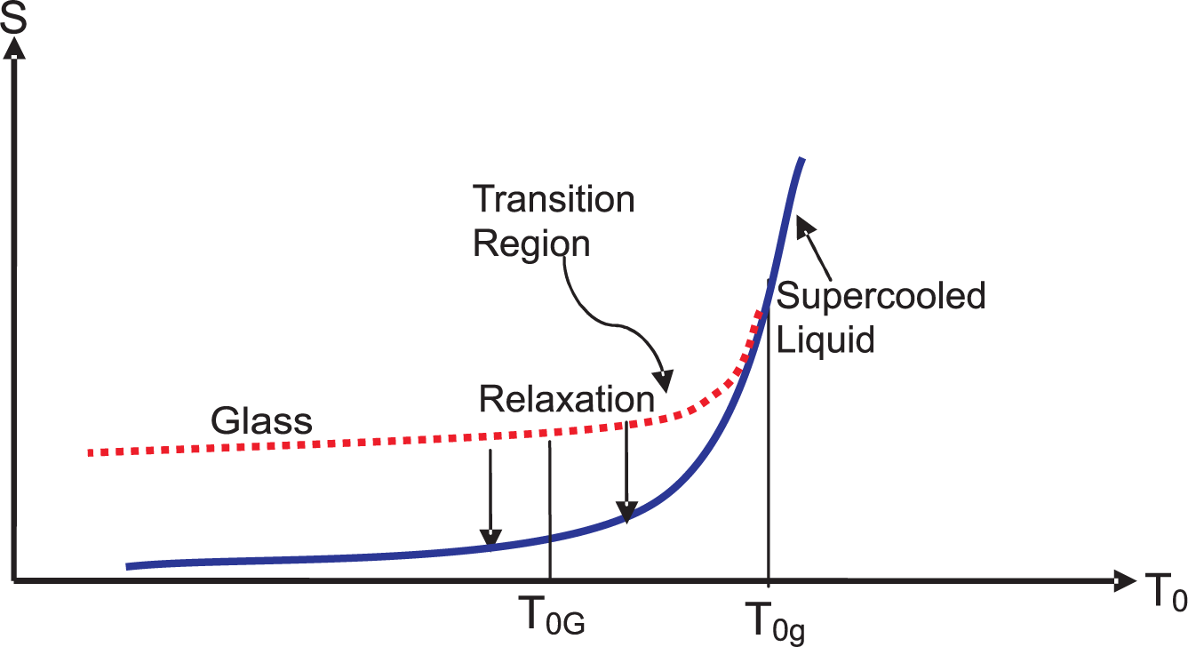
4. Vitrification and the Residual Entropy

As an application, we apply the above approach to vitrification, which is a prime example of an irreversible process going on at low temperatures. It is here one encounters the residual entropy, which will prove extremely useful in clarifying the confusion regarding which microstates are included in W in the Boltzmann entropy in Equation (39). Because of its importance, we briefly review vitrification. Normally, the process is carried out at some (not necessarily a fixed) cooling rate as follows but keeping the pressure P0 of the medium fixed. The temperature of the medium is isobarically lowered by some small but fixed ΔT0 from the current value to the new value, and we wait for (not necessarily fixed) time τobs at the new temperature to make an instantaneous measurement on the system before changing the temperature again. The choice of τobs ensures that at temperatures above the melting temperature T0M, the system is a liquid in equilibrium, which can be supercooled below T0M to give rise to a supercooled liquid. At some lower temperature T0g, see Figure 4, the equilibration time τeq, which continuously increases as the temperature is lowered, becomes equal to τobs. Just below T0g, the entropy of the system falls out of constrained equilibrium26 and follows the dotted curve, but the structures in the supercooled liquid are not yet frozen. They “freeze” at a lower temperature T0G (not too far from T0g) to form an amorphous solid with a viscosity close to 1013 poise.
This solid is identified as a glass (GL). The location of both temperatures depends on the rate of cooling, i.e., on τobs. Compared to the glass, the supercooled liquid (SCL) is in constrained equilibrium [70,71], and its entropy is shown by the continuous curve in Figure 4). Over the glass transition region between T0G and T0g, the nonequilibrium liquid (dotted curve) gradually turns from SCL at or above T0g into a glass at or below T0G [58]. Over this region, thermodynamic quantities such as the volume or the enthalpy change continuously but slowly during cooling. In addition, they also undergo relaxation towards SCL even if the temperature of the medium is held fixed; see the two downward vertical arrows. It is commonly believed that SSCL vanishes at absolute zero (SSCL(0) ≡ 0).
We bring the glass forming system Σ, which is at time t1 in a medium at temperature T01 (we will not explicitly exhibit P0 in this section) in a macrostate 1, into a medium at a lower temperature T02 at time t2, where it happens to be macrostate 2 via an irreversible vitrification process P 12 . We have along P 12
S ( 2 ) P 12 = S ( 1 ) + P 12 d e S + P 12 d i S ,
which follows from Equation (26). A discontinuous change in the entropy is ruled out from the continuity of the Gibbs free energy G and the enthalpy H in vitrification proved elsewhere [35]. Since the second integral in Equation (45) is always positive, we conclude that
S ( 2 ) > S ( 1 ) + T 01 T 02 C P d T 0 / T 0 .
For an equilibrium macrostate 1 such as a liquid at or above T0 = T0M, S(1) = Seq(eq1). The residual entropy SR of the glass, which is the entropy S(0) at absolute zero (T02 = 0), can be expressed as
S R S ( 0 ) > S expt ( 0 ) S ( T 0 ) + T 0 0 C P d T 0 / T 0 .
It follows from this that SR must be strictly larger than the measured27 Sexpt(0) in the vitrification process; note that we have put no restriction on the nature of the states along the dotted curve in the above derivation. The difference SRSexpt(0) would be larger, more irreversible the process is. The quantity Sexpt(0) can be determined calorimetrically by performing a cooling experiment. We take T01 to be the melting temperature T0M, and uniquely determine the entropy of the supercooled liquid at T0M by adding the entropy of melting (fusion) to the crystal (CR) entropy SCR(T0M) at T0M. The latter is obtained in a unique manner by integration along a reversible path from T0 = 0 to T0 = T0M:
S CR ( T 0 M ) = S CR ( 0 ) + 0 T 0 M C P , CR , d T 0 / T 0 ,
here, SCR(0) is the entropy of the crystal at absolute zero, which is traditionally taken to be zero in accordance with the third law and which we assume here, and CP,CR(T0) is the equilibrium isobaric heat capacity of the crystal. This then uniquely determines the entropy of the liquid to be used on the right hand side in Equation (47).
Experiment evidence for a non-zero value of Sexpt(0) is abundant as discussed by several authors [72,73,7582] among others; various textbooks [70,71] also discuss this issue. The strict inequality proves immediately that the residual entropy cannot vanish for glasses.

5. Statistical Entropy for an Isolated System with a Single Component Sample Space

The discussion in the last two sections has been about the thermodynamic entropy with no mention of microstates, component confinement in microstate space, etc., even though we have discussed vitrification in which a system can find itself among many disjoint components. We now turn to these topics as we provide a very general formulation of the statistical entropy.

5.1. General Derivation of the Statistical Entropy

The formulation is completely independent of the nature of dynamics in the system. The use of classical Newtonian dynamics at the microscopic level in identifying entropy was first initiated by Boltzmann [61,62] and has been a very active approach since then;28 see for example, Lebowitz [55,56]. The use of quantum dynamics was initiated by von Neumann [18] and has also been a very active approach, e.g., [33,42,43,64]. Despite this, it is important to investigate if it is possible to identify statistical entropy without the use of any dynamics. This is highly desirable as the dynamics, when extremely slow such as at low temperatures or in glasses, can result in the microstate space to consist of disjoint components in the system gets confined over the duration of τobs. The dynamics requires the temporal average of all the quantities over a period of time → ∞ (really larger than τeq). During component confinement, the dynamics does not allow the system to explore microstates belonging to disjoint components. Under this condition, if all physical quantities including the entropy are given by their temporal averages, then they should be governed by the particular component in which the system is found to be trapped; see the discussion in Section 1 and the footnote 10.
In contrast, Gibbs [10] introduced the ensemble average at each instant. The approach does not require any temporal average or dynamics. This issue was discussed elsewhere [72], where it was concluded that the temporal average is not suitable when τobs between successive measurements is not very large (τobs < τeq). The ensemble is found to represent all microstates even in the presence of confinement. It was also concluded that the ensemble average is always applicable. We will review this discussion and provide a clear evidence of the above conclusion when we discuss the issue of the residual thermodynamic entropy and its connection with the statistical entropy in Section 7. In addition, not bringing dynamics into consideration provides an opportunity to settle the dispute regarding the meaning of microstates counted in W; see the footnote 10. The correct interpretation will be found to be consistent with the ensemble average of Gibbs. This then reveals the true meaning of microstates counted in W.
Our approach will also demonstrate the statistical entropy to be a statistical average over microstates. Thus, it is not defined for a single microstate in our approach as is commonly done in stochastic thermodynamics [1416]. Our derivation is based on the Fundamental Axiom presented in Section 1, and requires (mentally) preparing a large number of samples at a given instant t, all specified by Z(t) [52]. How this can be done even though the internal variables are not controllable by the observer will become clear below. The samples represent microstates with nonzero probabilities. It is clear that even for a glass, there is no restriction that the samples all refer to the same component of the microstate space. Indeed, different sample will belong to different components and the collection of samples will represent all components as discussed above.
We introduce some useful notations to simplify the derivation. We consider a macrostate (t) ≡ (Z(t)) of a body Σ at a given instant t. In the following, we suppress t unless necessary. The macrostate (Z) refers to the set of microstates m = {mk} and their probabilities p = {pk}.29 For the computation of combinatorics, the probabilities are handled in the following abstract way. We consider a large number N = C W ( Z ) of independent samples of Σ, with C some large constant integer and W(Z) the number of distinct microstates mα that occur in (Z) with non-zero probabilities. We will use Γ(Z) to denote the microstate space spanned by these mks, which is assumed to be a single component in this section. Because of the restriction pα(t) > 0, the set m is determined by Z and will be denoted by m(Z) if clarity is needed.
For the isolated system Σ0, we add a suffix 0 to the various system quantities introduced above. Let N 0 α ( t ) denote the number of samples in the m0α-microstate so that
0 < p α ( t ) = N 0 α ( t ) / N 0 1 ; α = 1 W 0 ( Z 0 ) N 0 α ( t ) = N 0 .
The above sample space is a generalization of the ensemble introduced by Gibbs, except that the latter is restricted to an equilibrium system, whereas our sample space refers to the system in any arbitrary state so that pα may be time-dependent. The (sample or ensemble) average of some quantity Q0 over these samples is given by
Q ¯ 0 α = 1 W 0 ( Z 0 ) p α ( t ) Q 0 α , α = 1 W 0 ( Z 0 ) p α ( t ) 1 ,
where Q0α is the value of Q0 in m. As the samples are independent of each other, we can treat the samples to be the outcomes of some random variable, the macrostate 0(t). This independence property of the outcomes is crucial in the following, and does not imply that they are equiprobable. The number of ways W 0 to arrange the N 0 samples into W0(Z0) distinct microstates is
W 0 N 0 ! / α N 0 α ( t ) ! .
Taking its natural log to obtain an additive quantity per sample
S 0 ln W 0 / N 0 ,
and using Stirling’s approximation, we see easily that S 0, which we hope to identify later with the entropy S0(t), can be written as the average of the negative of η(t) ≡ ln p(t), what Gibbs [10] calls the index of probability:
S 0 ( Z 0 ( t ) , t ) η ( t ) ¯ α = 1 W 0 ( Z 0 ) p α ( t ) ln p α ( t ) ,
where we have also shown an explicit time-dependence for the reason that will become clear below.30 The above derivation is based on fundamental principles and does not require the system to be in equilibrium; therefore, it is always applicable. To the best of our knowledge, even though such an expression has been extensively used in the literature, it has been used without any derivation; one simply appeals to this form by invoking it as the information entropy; however, see Section 10.
Because of its similarity in form with S G ( c ) in Equation (20), we will refer to S 0 ( Z 0 ( t ) , t ) as the Gibbs statistical entropy from now on. As the entropy for a process in which the system is always in IEQS can be determined by integrating the Gibbs fundamental relation in Equation (28), we can compare it with the statistical entropy introduced above. However, such an integration is not possible for a process involving states that are arbitrary (not in internal equilibrium). Therefore, it is not possible to compare S 0 ( t ) with the corresponding thermodynamic entropy only because the value of the latter cannot be determined.
We refer the reader to several proofs in the literature [11,12,52,64,83,84] establishing that S 0 ( t ) satisfies Equation (25). The maximum S 0 ( t ) for given Z 0 ( t ) occurs when m0α are equally probable:
p α ( t ) p α , int . eq 1 / W 0 ( Z 0 ) , m α Γ 0 ( Z 0 ) .
In this case, the explicit time dependence in S 0 ( t ) disappears and we have
S 0 , max ( Z 0 ( t ) , t ) = S 0 ( Z 0 ( t ) ) = ln W 0 ( Z 0 ( t ) ) ,
which is identical in form to the Boltzmann entropy in Equation (18) for an isolated body in equilibrium, except that the current formulation has been extended to an isolated body out of equilibrium; see also Equation (39). The statistical entropy in this case becomes a state function. The only requirement is that all microstates in m0(Z0) be equally probable. This is the extension of the maximum entropy principle to IEQSs first proposed by Gibbs [10] for EQSs and extensively studied later by Jaynes [8587].
Let us consider a macrostate specified by some X0 and the set m ¯ 0 consisting of microstates { m ¯ α }. Let { p ¯ α ( t ) } denote the set of probabilities for m ¯ 0. Applying the above formulation to this macrostate, we obtain
S 0 ( X 0 , t ) α = 1 W 0 ( X 0 ) p ¯ α ( t ) ln p ¯ α ( t ) , α = 1 W 0 ( X 0 ) p ¯ α ( t ) 1 ,
as the statistical entropy of this macrostate, where W0(X0) is the number of distinct microstates should be obvious that
W 0 ( X 0 ) ξ 0 ( t ) W 0 ( Z 0 ( t ) ) .
Again, under the equiprobability assumption
p ¯ α ( t ) p α , eq = 1 / W 0 ( X 0 ) , m ¯ α Γ 0 ( X 0 ) ,
Γ0(X0) denoting the space spanned by microstates { m ¯ α }, S 0 ( X 0 , t ) takes its maximum possible value
S 0 , max ( X 0 , t ) = S 0 ( X 0 ) = ln W 0 ( X 0 ) ,
which from Section 2.2 is identical the thermodynamic entropy S0eq for an isolated body in equilibrium. The maximum value occurs at tτ0eq. It is evident that
S 0 [ Z 0 ( t ) , t ] S 0 [ Z 0 ( t ) ] S 0 ( X 0 ) ;
compare with Equation (34) by replacing Z ¯ 0 with Z0 and Z0 with X0 to obtain the above inequalities.
The anticipated identification of nonequilibrium thermodynamic entropy with S 0 under some restrictions allows us to identify S 0 as the statistical entropy formulation of the thermodynamic entropy. From now on, we will refer to the general entropy in Equation (52) in terms of microstate probabilities as the time-dependent Gibbs formulation of the entropy or simply the Gibbs entropy, and will not make any distinction between the statistical and thermodynamic entropies. Accordingly, we will now use the standard symbol S0 for S 0 for the rest of the work, unless clarity is needed.
We will refer to S0(Z0(t)) in terms of W0(Z0(t)) in Equation (53) as the time-dependent Boltzmann formulation of the entropy or simply the Boltzmann entropy [55,56], whereas S0(X0) in Equation (55) represents the equilibrium (Boltzmann) entropy. It is evident that the Gibbs formulation in Equations (52) and (54) supersedes the Boltzmann formulation in Equations (53) and (55), respectively, as the former contains the latter as a special limit. However, it should be also noted that there are competing views on which entropy is more general [42,43,55,56]. The continuity of S0(Z0, t) (except in the thermodynamic limit) follows directly from the continuity of pα(t). The existence of the statistical entropy S0(Z0, t) follows from the observation that it is bounded above by ln W0(Z0) and bounded below by 0, see Equation (53).
It should be stressed that W is not the number of microstates of the N replicas; the latter is given by [ W 0 ( Z 0 ) ] N. Thus, the entropy in Equation (51) should not be confused with the Boltzmann entropy, which would be given by N. It should be mentioned at this point that Boltzmann uses the combinatorial argument to obtain the entropy of a gas, see Equation (21), resulting in an expression similar to that of the Gibbs entropy in Equation (20) except that the probabilities appearing in his formulation represents the probability of various discrete states of a particle.

6. Statistical Entropy for an Interacting System with a Single Component Sample Space

6.1. Statistical Entropies of the System and Medium

The system must be treated as interacting (with a medium) if any measurements have to be performed on it. Using the above formulation of S0(Z0(t), t), see Equation (52), we have determined [36] the statistical formulation of the entropy for a system Σ, which is a small but macroscopically large part of Σ0; see Figure 1b and Equation (43). It is assumed that the system and the medium are quasi-independent so that S0(t) ≡ S0(Z0(t),t) can be expressed as a sum of entropies S(t) ≡ S(Z(t),t) and S ˜ ( t ) S ˜ ( Z ˜ ( t ) ) of the system and the medium, respectively; see [36] for the derivation, which we omit here as it is straightforward. The two statistical entropies are given by identical formulations
S ( t ) = k p k ( t ) ln p k ( t ) , S ˜ ( t ) = k p ˜ k ( t ) ln p ˜ k ( t ) ,
respectively. Here, mk with probability pk > 0 denotes a microstate of Σ and m ˜ k with probability p ˜ k > 0 that of the medium. In the derivation [36], we neither assume the medium nor the system to be in internal equilibrium. Thus, the above formulations of statistical entropies are valid under all conditions. However, the formulation will not remain valid if the two systems are not quasi-independent; in that case, we must account for the entropy contribution due to their mutual interactions. The same will also be true of the thermodynamic entropies.

6.2. Statistical Entropy as a State Function: IEQS

For a system in IEQS, its statistical entropy S(t) must be maximized under the constraints imposed by the medium; compare with Gibbs [10] and Jaynes [8587] for EQSs with no internal variables. The constraints we need to satisfy are on the fixed average values of the state variables:
Z ( t ) = k Z k p k ,
where Zk is the value of Z in mk. The condition for an IEQS is obtained by varying pk. Using the Lagrange multiplier technique, it is easy to see that the condition for this in terms of the Lagrange multipliers whose definitions are obvious is
ln p k = λ + λ · Z k ;
the scalar product is over the elements in the set Zk. It now follows that
S = λ + λ · Z ( t ) ,
using the above scalar product. We identify the Lagrange multipliers by observing that
d S = λ · d Z .
Comparing this relation with the Gibbs fundamental relation for the system in Equation (36), we find
λ p ( S / Z p ) .
Accepting this identification now allows us to conclude that the statistical entropy S(t) of the interacting system in Equation (57) is no different than thermodynamic entropy of the same system in IEQS up to a constant. The constant can be determined by the use of the Nernst’s postulate for both entropies to ensure that they are numerically identical and proves the following claim:
Claim 5. The two entropies are identical everywhere for an interacting system in IEquations
The significance of λ is quite obvious. In IEQS, it is given by
λ = S ( S / Z ) · Z ( t ) .
In equilibrium, the Lagrange multipliers associated with the internal variables vanish and Equation (60) reduces to
d S eq = λ eq · d X .
A special case of such a system is the (equilibrium) canonical ensemble of Gibbs.

6.3. Statistical Entropy not a State Function: ANEQS

The thermodynamic entropy for an ANEQS cannot be measured or computed. Thus, while the statistical entropy can be computed in principle in all cases, there is no way to compare its value with the thermodynamic entropy in all cases. Thus, no comment can be made about their relationship in general. However, as discussed in Section 3.8, we are able to express the non-state thermodynamic entropy of an inhomogeneous body in terms of the state entropies of its quasi-independent subsystem. It is easy to see that both entropies are identical. Furthermore, when the system is in a homogeneous ANEQS, the inequalities in Equations (56) and (34) also shows the deep connection between the two entropies. However, as arbitrary states occur because of an incomplete specification of the NEQS, the problem is more of an incomplete specification. We can find an extended set Z ¯ for a complete specification of the macrostate so that the entropy becomes a state function. Thus, we conjecture the following:
Conjecture 1. As the two entropies are the same when the homogeneous body is in IEQS or when it is in an inhomogeneous ANEQS for which various quasi-independent subsystems are in IEQSs, the thermodynamic entropy is no different from its statistical analog for any NEQS.
The conjecture allows a computational method to determine the thermodynamic entropy for any NEQS.

7. Statistical Entropy with Component Confinement

The consideration of dynamics when the sample (also known as the microstate or phase) space has a single component has played a pivotal role in developing the kinetic theory of gases [55,56,62], where the interest is at high temperatures. As dynamics is very fast here, it is well known that the ensemble entropy agrees with its temporal formulation. However, at low temperatures, where dynamics becomes sluggish as in a glass [57,58], the system can be confined into disjoint components. This occurs when the observational time scale τobs becomes shorter than the equilibration time τeq; see also Section 4.
Confinement at a phase transition such as a liquid-gas transition is well known in equilibrium statistical mechanics [4,52,72]. It also occurs when the system undergoes symmetry breaking such as during magnetic transitions, crystallizations, etc. However, confinement can also occur under nonequilibrium conditions. The issue has been recently considered by us [52], where only energy as an observable was considered. We again focus on an isolated system Σ0. The discussion is easily extended to the present case when confinement occurs for whatever reasons into one of the thermodynamically significant number31 of disjoint components Γ, λ = 1, 2, 3⋯, C 0, each component corresponding to the same set Z0 (we suppress the dependence for simplicity), respectively. Such a situation arises, for example, in Ising magnets at the ferromagnetic transition., where the system is either confined to Γ0+ with positive magnetization or Γ0− with negative magnetization. Even a weak external magnetic field |H| → 0, that we can control as an observer, will allow the system to make a choice between the two parts of Γ0. It just happens that in this case C = 2 and is thermodynamically insignificant.
The situation with glasses or other amorphous materials is very different [57]. We again focus on an isolated system Σ0. In the first place, Γ0 is a union of thermodynamically significant number C 0 e c 0 N 0 , c 0 > 0, disjoint components. In the second place, there is no analog of a symmetry breaking field. Therefore, there is no way to prepare a sample in a given component Γ. Thus, the samples will be found in all different components. As there is no symmetry breaking field, there is no harm in treating the glass as an isolated system. Taking into consideration disjointness of the components generalizes the number of configurations in Equation (50) to
W 0 N 0 ! / λ , α λ N 0 α λ ( t ) ! ,
where N 0 α λ denotes the number of sample in the microstate m0αλ in the λ-th component. In terms of p α λ = N 0 α λ ( t ) / N 0, this combination immediately leads to
S 0 ( t ) ln W 0 / N 0 = λ α λ p α λ ( t ) ln p α λ ( t ) ,
for the statistical entropy of the system and has already been used earlier [52] by us; see Section 4.3.3 there. From what has been said above, this statistical entropy is also the thermodynamic entropy of a IEQS under component confinement for which both entropies are state functions of Z0. Therefore, as before, we take S 0 to be the general expression of the nonequilibrium thermodynamic entropy and use S0 in place of S 0.
It should be stressed that the number of microstates that appear in S 0 ( t ) has an explicit sum over all components, and not just a single component that would be the case if there were a symmetry breaking field to prepare the body in a particular component. This observation will prove important below when making connection with glasses.
In terms of p λ ( t ) α λ p α λ ( t ), it is easy to see [52] that
S 0 ( t ) = λ p λ ( t ) S 0 λ ( t ) + S 0 C ( t ) .
The entropy S(t) of the component Γ in terms of the reduced microstate probability p ^ α λ p α λ / p λ is
S 0 λ ( t ) = α λ p ^ α λ ( t ) ln p ^ α λ ( t )
so that it is its average over all components. The second term represents the component entropy and is given by
S 0 C ( t ) = λ p λ ( t ) ln p λ ( t ) ,
The same calculation for an interacting system will result in an identical formulation for the entropy S(t) as in Equation (65) and other quantities. For S(t), we have
S ( t ) = μ k μ p k μ ( t ) ln p k μ ( t ) ,
where the sum over μ is over disjoint components T d i ( Q ) S = ( T 0 T ) d e S, for the system, and kμ represents a microstate in the μth component. The component entropy S C ( t ) is given by
S C ( t ) = μ p μ ( t ) ln p μ ( t ) ,
with the sum over disjoint components μ for the system. We now apply this formulation to a glass, which is now treated as an interacting system. As noted above, the number of microstates that appear in S(t) belong to all C components. At absolute zero, only the lowest lying (in energy) microstate in each component will be occupied, which we take to be non-degenerate. In this case, the analog p ^ k μ of p ^ α λ for the μth component is p ^ k μ = 1. Thus, the analog Sμ(t) of S(t) is strictly zero: Sμ(t) = 0. It then follows that at absolute zero, S ( t ) = S C ( t ) determines the residual entropy of any glassy NEQS.
If it happens that S(t) in Equation (68) is restricted to a sum over a single component, then SC(t) = 0 and the residual entropy will always vanish for all NEQSs. This means that the number of microstates that appears in the Boltzmann formulation will correspond to Wμ(Z), the number of microstates in the μth component in which the glass appears to confined. As the glass cannot visit microstates belonging to other components in the duration τobs, this scenario suggests that the not all microstates determine the entropy of the system. However, as the experimental evidence is quite strong that the residual entropy is not zero as discussed in Section 4, we must conclude that it is not Wμ(Z) but all microstates in all components determines the residual entropy, which is given by the absolute zero value of SC(t) in Equation (69). If all components are equally probable, then p μ ( t ) = 1 / C ( 0 ), with C ( 0 ) representing the number of components at absolute zero, then the residual entropy of a glass in IEQS is given by
S R = ln C ( 0 ) > 0.
Finally, the calorimetrically measured (see footnote 27) non-zero entropy Sexpt(0), which is a lower bound on SR, see Equation (47), allows us to finally settle the meaning of W that appears in the Boltzmann formulation.
Claim 6. W that appears in the Boltzmann formulation represents all microstates with non-zero probabilities regardless of whether they can be accessed by the system during τobs.

8. Semi-Classical Approximation in Phase Space for S

The analog of a quantum microstate in classical statistical mechanics is normally obtained by recognizing that in the adiabatic approximation,32 each small phase space cell of volume element dxc(= dpdq in terms of generalized coordinates q and momenta p) of size hs corresponds to a microstate [4,12], where s is the degrees of freedom of the system. The latter follows from the Bohr-Sommerfeld quantization rule for a periodic motion. The adiabatic approximation requires the parameters characterizing the system to vary extremely slowly. We will assume one such parameter λ (such as the volume V) so that [90] τλ << λ, where τ is the period of oscillation for constant λ; the system would be isolated in the latter case. In the above approximation, the energy of the system will vary very slowly and can be taken to be constant over a period of oscillation. The action taken over the closed path for the constant value of λ and the energy is quantized [17]: ∫ pdq = (n + 1/2)h. This observation is the justification of the above cell size of a classical microstate. Thus, the number of “classical” microstates is given by W = ΔΓ/hs, where ΔΓ is the phase space volume corresponding to the system. This allows us to divide the phase space into W cells, index by k, of volume dxk = dxc and “centered” at xk at some time which we call the initial time t = 0. We will denote the evolution of the cell at time t by the location of its “center” xk(t) and its volume element dxk(t). In terms of the distribution function f(x, ξ, t) in the phase space, which may depend on the internal variables, the kth microstate probability therefore is given by
p k ( t ) f ( x k , ξ k , t ) d x k ( t ) .
Evidently,
k f ( x k , ξ k , t ) d x k ( t ) = 1
at all times. The entropy and the average of any observable O(x, t) of the system are given by
S ( t ) k f ( x k , ξ k , t ) d x k ( t ) ln [ f ( x k , ξ k , t ) d x k ( t ) ] ,
O ¯ ( t ) k O ( x k , t ) f ( x k , ξ k , t ) d x k ( t ) ,
the sum being over all W microstates. While it is easy to see that continuum analogs for Equations (71) and (72b) are easily identified, this is not so for the entropy in Equation (72a) [88,89]. However, it should be obvious that Sf in Equation (22) cannot be a candidate for the statistical entropy S(t).
It is well known [17] that the system in the adiabatic limit remains in the same quantum state. For Hamiltonian dynamics, the conservation of the phase space cell volume under evolution ensures dxk = dxc for each cell so that x ˙ = 0. This results in the incompressibility of the phase space. In equilibrium, f(xk, t) is not only uniform but also constant, and we conclude from Equation (71) that this value is f = 1/ΔΓ. Accordingly, pk = 1/W in equilibrium as expected and we obtain the equilibrium entropy Seq = ln W.
The situation is far from clear for nonequilibrium states. The system is no longer restricted to be in the same microstate, which means that the microstate energy is no longer a constant and the phase space trajectory is no longer closed. Thus, the suitability of the Bohr-Sommerfeld quantization is questionable, and care must be exercised to identify the microstates. We will adopt the following prescription. We consider some EQS (uniform f(x)) of the isolated system to identify the cell volume dxc = hs. Once the identification has been done, we will no longer worry about its relationship with hs, and only deal with the cells. We then follow the evolution of each cell in time in a nonequilibrium process during which x ˙ = 0 may or may not hold. Thus the volume of each cell may no longer be constant. The process may also result in changes in f [91]. Indeed, it is quite possible that f diverges at the same time that dxc vanishes [92]. However, their product, which determines the microstate probability, must remain strictly bounded and ≤ 1. In particular, as the cell volume shrinks to zero, f must diverge to keep the product bounded. Thus, the divergence [93,94] of f alone does not imply that the entropy diverges to negative infinity.
This is easily seen by the following 1-d damped oscillator, the standard prototype of a dissipative system [90]: x ¨ + 2 κ x ˙ + ω 0 2 x = 0 with a (positive) damping coefficient, which is chosen such that κ > ω0 just for simplicity. We have the case of aperiodic damping. We will only consider the long time behavior. It is easy to see that in this limit ( κ = κ + κ 2 ω 0 2 )
d x c exp ( 2 κ t ) , f exp ( + 2 κ t ) ,
and their product remains bounded, as expected.

9. 1-d Tonks Gas: A simple Continuum Model

A careful reader would have realized by this time that the proposed entropy form in Equation (52) is not at all the same as the standard classical formulation of entropy, such as for the ideal gas, which can be negative at low temperatures or at high pressures. The issue has been discussed elsewhere [95] but with a very different perspective. Here, we visit the same issue from yet another perspective that allows us to investigate if and how the entropy in continuum models is related to the proposed entropy in this work. For this, we turn to a very simple continuum model in classical statistical mechanics: the Tonks gas [96,97], which is an athermal model and contains the ideal gas as a limiting case when the rod length l vanishes. We will simplify the discussion by considering the Tonks gas in one dimension. The gas consists of r impenetrable rods, each of length l lying along a line of length L. We will assume r to be fixed, but allow l and L to change with the state of the system determined by its temperature, pressure, etc. The configurational entropy per rod determined by the configurational partition function is found to be [97]
s c = ln [ e ( v l ) a ] ,
where υ is the “volume” available per rod L/r and a is a constant that has the dimension of length to make the entropy and the corresponding configurational partition function33
Z c = 1 a r exp ( ϕ ( x 1 , x 2 , x r ) / T ) d x 1 d x 2 d x r
dimensionless. The function ϕ represents the overlap potential, which is zero when no rods overlap and becomes infinitely large whenever there is an overlap [97]. The temperature of the gas is denoted by T, which is determined by the distribution of momenta of various rods.34 As we will be relating Tonks gas to a lattice model, we will only consider the configurational entropy in the rest of the section. The configurational entropy is obtained by dividing T ln Zc by T. Even though sc is derived for an equilibrium Tonks gas, it is easy to see from the nature of the microstate probabilities pk in Equation (58) that the same result also applies for the gas in internal equilibrium whose temperature is T. The set Z of state variables includes E, L, r, l and ξ. All other extensive quantities will in general be functions of Z.
The entropy vanishes when υ = l + 1/ae and becomes negative for all l < υ < l + 1/ae. Indeed, it diverges to −∞ in the incompressible limit υ = l. This is contrary to the statistical entropy in the Boltzmann approach (cf. Equation (18)) or the Gibbs approach (cf. Equation (52)), +which can never be negative. Can we reconcile the contradiction between the continuum entropy and the current statistical formulation?
We now demonstrate that the above entropy for the Tonks gas is derivable from the current statistical approach under some approximation, to be noted below, by first considering a lattice model for the Tonks gas and then taking its continuum limit. It is in the lattice model can we determine the number of microstates. In a continuum, this number is always unbounded (see below also). We consider a 1-d lattice Λf with Nf sites; the lattice spacing, the distance between two consecutive sites, is given by δ. We take Nf >> 1 so that Lf = Lrl = (Nf − 1)δNfδ is the length of the the lattice Λf. Evidently, Lf is a function of observables L, r, and l, it does not depend on ξ. Despite this, there is no reason to assume that Nf and δ individually do not depend on E and ξ; only their product is independent. In general, we expect Nf and δ to depend on Z.
We randomly select r sites out of Nf. The number of ways, which then represents the number of configurational microstates, is given by
W c = N f ! / r ! ( N f r ) ! .
After the choice is made, we replace each selected site by λ + 1 consecutive sites, each site representing an atoms in a rod, to give rise to a rod of length lλδ. The number of sites in the resulting lattice Λ is
N = N f + r λ
so that the length of Λ is given by L = Lf + rl = (N − 1)δ since N >> 1. Again, there is no reason to assume that N and δ individually do not depend on Z as above.
We introduce the number densities φf = r/Nf, ρf = r/Nfδr/Lf and ρ = r/r/L. A simple calculation shows that S = ln Wc is given by
S = N f [ ρ f δ ln ρ f δ + ( 1 ρ f δ ) ln ( 1 ρ f δ ) ] .
This result can also be obtained by taking the athermal entropy for a monodisperse polymer solution a Bethe lattice [98] by setting the coordination number q to be q = 2. We now take the continuum limit δ → 0 for fixed ρf and ρ, that is fixed Lf and L, respectively. In this limit, (1 − ρfδ) ln(1 − ρfδ) ≈ −ρfδ, and we find
S = r ln ( e / ρ f δ ) .
The continuum limit of S using the Boltzmann approach has resulted in a diverging entropy regardless of the value of ρf [95], a well known result. Using the arbitrary constant a of Equation (73) results in
S / r = ln ( e / ρ f a ) ln ( δ / a ) ,
in which the first term remains finite in the continuum limit, and the second term contains the divergence.35 The diverging part, although explicitly independent of ρf, still depends on the state of the gas through δ, and cannot be treated as a constant unless we assume δ to be independent of the state of the gas. It is a common practice to approximate the lattice spacing δ as a constant. In that case, the diverging term represents a constant that can be subtracted from S/r. Recognizing that 1/ρf = υl, we see that the first term in Equation (75) is nothing but the entropy of the Tonks gas in Equation (73). The equivalence only holds in the state independent constant δ approximation.
As the second term above has been discarded, the continuum entropy sc also has no simple relationship with the number (≥ 1) of microstates in the continuum limit, which means that the continuum entropy cannot be identified as the Boltzmann entropy in Equation (55). To see this more clearly, let us focus on the centers of mass of the rods; they can be thought of as representing the r sites that were selected in Λf. Each of the r sites xk, k = 1, 2,⋯, r, is free to move over Lf. The adimensional volume |Γf|, also called the probability and denoted by Z (not to be confused with the the partition function) by Boltzmann [55,56,63], of the corresponding phase space Γf is L f r / a r. However, contrary to the conventional wisdom [55,56], ln |Γf| does not yield sc. The correct expression is given by the Gibbs-modified adimensional volume |Γf|/r!, i.e.,
1 r ! a r L f r .
The presence of r! is required to restrict the volume due to indistinguishability of the rods à la Gibbs. For large r, this quantity correctly gives the entropy sc. However, this quantity is not only not an integer, it also cannot be always larger than or equal to unity, as noted above.

10. Summary and Discussion

The current work is motivated by a desire to understand the relationship between thermodynamic and statistical entropies. We have briefly reviewed the thermodynamic entropy and several important statistical entropies in Section 2. Of the latter, we pay close attention to the Boltzmann and Gibbs entropies that have played a major role in contemporary statistical thermodynamics. While these entropies and their equivalence with thermodynamic entropies are well understood in equilibrium for ergodic systems, it is not so obvious that the equivalence also holds off-equilibrium. Extension to nonequilibrium states gives rise to new and important technical problems, requires clarification of some confusion in the field, but also results in establishing the Clausius equality dQ = TdS which gives rise to some simplification of extreme importance; see point (6) below.
  • We need to formulate the concept of a state, state variables and state functions. We discuss these issues and the behavior of nonequilibrium thermodynamic entropy in Section 3, where we follow the recent approach initiated by us [3539]. In particular, we discuss the role of internal variables that are needed to specify the (macro)state of a NEQS. Without internal variables, we cannot introduce the concept of a macrostate for an isolated system (see Section 3.1 and an interacting system (see Section 3.4). Thus, state variables include extensive observables (see footnote 11) and internal variables (see footnote 17) to specify a macrostate. The thermodynamic entropy is a state function for IEQS but a non-state function for ANEQS. The concept of internal equilibrium to characterize IEQSs [3539] is based on the fact that state variables uniquely specify homogeneous macrostates. We point out its close similarity with the concept of equilibrium; see Section 3.6. The relationship of ANEQSs to IEQSs is similar to that of NEQSs to EQSs. In particular, we show how the entropy can be calculated for any arbitrary nonequilibrium process whose end states are IEQSs. We discuss various aspects of internal equilibrium and show how the entropy of an inhomogeneous system in ANEQS can be determined provided each of its subsystems are in internal equilibrium; see Section 3.8. A uniform body not in internal equilibrium with respect to a smaller set Z(t) of state variables can be made in internal equilibrium by extending the set of state variables. This justifies our claim in footnote 8. The vitrification process is reviewed in Section 4 where we introduce the concept of the residual thermodynamic entropy SR.
  • We provide a first principles statistical formulation of nonequilibrium thermodynamic entropy for an isolated system in terms of microstate probabilities without the use of any dynamical laws36 in Section 5. The formulation is based on the Fundamental Axiom and is valid for any state of the body. We use a formal approach (frequentist interpretation of probability) by extending the equilibrium ensemble of Gibbs to a nonequilibrium ensemble, which is nothing but a large number N 0 of (mental) samples of the body under consideration; we refer the ensemble as a sample space. The formal approach enables us to evaluate the combinatorics for a given set of microstate probabilities. The resulting statistical entropy is independent of the number of samples and depends only on the probabilities as is seen from Equations (52) and (64). Thus, the use of a large number of samples is merely a mathematical formality and is not required in practice. We have shown that in equilibrium, the statistical entropy is the same as the equilibrium thermodynamic entropy: S eq ( X ) = S eq ( X ). However, we have also shown that the statistical entropy is equal to the thermodynamic entropy in IEQS described by the state variables Z ( t ) : S IEQS ( Z ( t ) ) = S IEQS ( Z ( t ) ). The IEQSs correspond to homogeneous states of the body. The conclusion also remains valid for an inhomogeneous system in ANEQS whose subsystems are individually homogeneous and in different IEQSs. We cannot make any comment about the relationship between S ( Z ( t ) , t ) and S(Z(t),t) for the simple reason that there is no way to measure or calculate a non-state function S(Z(t),t). Despite this, when the system is in a homogeneous ANEQS, the inequalities in Equations (56) and (34) still show the deep connection between the two entropies. Therefore, the statistical entropy in this case can be used to give the value of the corresponding thermodynamic entropy. This then finally allows us to make Conjecture 1 in Section 6. The discussion is extended to the case where state space is multi-component such as in glasses in Section 7.
  • The second problem relates to the meaning of the number of microstates W that appears in the Boltzmann entropy. We have concluded in previous work [52,58] that temporal averages may not be relevant at low temperatures where component confinement occurs in of thermodynamically significant several disjoined components. The glass is formed when the system gets trapped in one of these components. Does W refer to the number of microstates within this component or to all microstates in all the components even though the glass is not allowed to probe these components over the observation period τobs < τeq? If dynamics is vital for the thermodynamics of the system, then it would appear that latter alternative should be unacceptable. Various reliable estimates for SR show that it is positive. Its positive value plays a very important role in clarifying the meaning of W. The answer is that W must contain all the microstates with non-zero probabilities in all disjoint components; see the Claim 6 in Section 7.
  • In Section 8, we briefly review the semi-classical approximation for the entropy by introducing cells in phase space, whose volume is hs under adiabatic approximation. Using the cell construction, we show that Sf in Equation (22) cannot represent the entropy of the system. We argue that for nonequilibrium states, f may diverge as the cell volume dxc → 0. However, the product fdxc must be strictly ≤ 1. We consider a simple example of a 1-d damped oscillator for which we show that the above conclusion is indeed valid. Thus, contrary to what is commonly stated, e.g., [92,94], the divergence of f does not mean that the entropy also diverges.
  • Thermodynamic entropy can become negative, but this is not possible for the statistical entropy. To clarify the issue, we consider a simple lattice model in Section 9, which in the continuum limit becomes the noninteracting Tonks gas. The latter model has been solved exactly and shows negative entropy at high coverage; see Equation (73). The entropy of the original lattice model is non-negative at all coverages and reduces to zero only when the coverage is full. It is found that one must subtract a term containing δ, the lattice spacing. By a proper subtraction, the lattice entropy has been shown to reproduce the continuum entropy in Equation (73) as δ → 0. It is a common practice to treat δ a constant, in which case the subtraction is harmless. However, there is no reason to assume δ to be state independent.
  • One encounters inequalities such as in Equation (2), which creates problems in determining the entropy calorimetrically; the calorimetric determination of deQ and T0 is not sufficient to obtain dS. In our approach based on internal variables [38,39], see in particular the discussion starting below Equation (3) and leading to Equation (6), we have dQ = deQ + diQ = T (t)dS(t), dW = deW + diW = P(t)dV(t) +⋯+ A(t) · dξ(t) so that the inequality dS > deQ/T0 is replaced by an equality dS = dQ/T (t). Thus, both dQ and dW are expressed in terms of the fields of the body defined in Equation (35). This provides for tremendous simplification as internal equilibrium is very similar in many respect to equilibrium; see Section 3.6 and Ref. [38,39].
  • For an isolated system in internal equilibrium (pα = p for ∀mα), just a single sample (or microstate) will suffice to determine the entropy as samples are unbiased. The entropy in this case is no different than the “entropy” − ln p of a single sample [52,55,56]:
    S ( t ) = ( p ln p ) W 0 = ln p = ln W 0 ,
    where W0 represents W0(Z0(t)) or W0(X0). The entropy of the “single” microstate in this case will always satisfy the second law for W0 continues to increase as the system relaxes.
  • However, this simplicity is lost as soon as the system is not in internal equilibrium. Here, one must consider averaging over all microstates to evaluate the statistical entropy, which must satisfy the second law. In contrast, the negative of the index of probability −η(t) used in Equation (52), which has also been identified as the microstate entropy in modern literature [1416], may increase or decrease with time. This is merely a consequence of probability conservation (see the second equation in Equation (49)), and is not related to second law, which refers to the behavior of the negative of the average index of probability.
  • Some readers may think that our statistical formulation is no different than that used in the information theory. We disagree. For one, there is no concept of internal variables ξ0 in the latter theory. Because of this, our approach allows us to consider three levels of description so that we can consider three different entropies S0(Z0(t),t), S0(Z0(t)) and S0(X0) satisfying the inequalities in Equation (56). The information theory can only deal with two levels of entropies. There is also no possibility of a residual entropy in the latter.
  • We should remark here that the standard approach to calculate nonequilibrium entropy is to use the classical nonequilibrium thermodynamics [3] or its variant, which treats the entropy at the local level as an equilibrium state function. Moreover, it can only treat an inhomogeneous system in a NEQS but not a homogeneous NEQS. Furthermore, the correlation length plays no role in determining the “elemental volume” over which local equilibrium holds [6] (p. 335). As no internal variables are required, it is different from our approach which exploits internal variables. Our approach is also different from those approaches in which the entropy is treated as a function of fluxes [9]. As fluxes depend strongly on how the system relates to the medium, they cannot serve as state variables for the system in our approach; see SP1 and the discussion following it.
We suggest that our statistical Gibbs formulation can be applied to any NEQS. However, as there does not appear at present a way to experimentally measure the thermodynamic entropy in an arbitrary NEQS, there is no hope to compare the two entropies in all cases. Therefore, our final conclusion is presented as a conjecture.

Acknowledgments

I thank Gian Paolo Beretta for his invitation to contribute this paper to this special issue based on topics discussed at the 12th Joint European Thermodynamics Conference, JETC2013, held in Brescia, Italy, July 1–5, 2013 and for various illuminating discussions. I am also indebted to Roberto Trasarti-Battistoni for various constructive comments that helped improve the manuscript significantly.
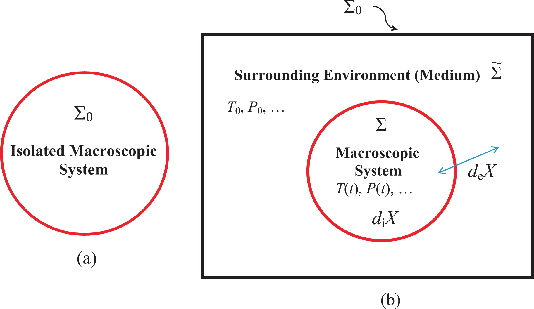
  • 1The number of these variables is determined by the nature of description of the system appropriate in a given investigation of it. In equilibrium, the entropy is a unique function of these variables, called the observables. It should be noted that extensivity does not imply additivity (sum of parts equals the total) and vice versa. As additivity plays a central role in our approach, we will restrict ourselves to only short-ranged interactions or screened long-ranged interactions such as the electrostatic interactions screened over the Debye length [4] (Sections 78–80). The interaction in both cases is tempered and stable [40] (p. 320). In addition, we require our system to be mechanically and thermodynamically independent from the medium, see Figure 1b, in the sense discussed later in Section 3.8; however, see [5].
  • 2This point is carefully discussed on pp. 8–9 in Ref. [36] and alluded to in Ref. [40].
  • 3The reversible entropy exchange deS always appears as an equality for any process (reversible or irreversible): deS = deQ/T0. In terms of the irreversible entropy diS ≥ 0 generated within the body, the entropy change is dSdiS + deS, which then results in the Clausius inequality dS > deS for an irreversible process. Furthermore, we will reserve the use of dQ in this review to denote the sum dQdiQ + deQ, where diQ is irreversible heat generated within the system due to internal dissipation.
  • 4Throughout this work, we only consider nonnegative temperatures of the medium.
  • 5The energy can only change by exchanges with the medium. As no internal process can change the energy, we have diE = 0 so that dE = deE. To understand the nature of diX, we need to consider an isolated system. It is easy to see that diV = 0, but diW, diN, etc. need not be zero.
  • 6Some of the physical significance of the entropy that will be discussed in the review are its identification as a macroscopic concept, its behavior in a spontaneous process, a possible state function, its relevance for thermodynamic forces and nonequilibrium thermodynamics, its equivalence with the statistical entropy that is always non-negative, its ability to explain the residual entropy, etc.
  • 7The number of papers and books on nonequilibrium entropy is so vast that it is not possible to do justice to all of them in the review. Therefore, we limit ourselves to cite only a sample of papers and books that are relevant to this work and we ask forgiveness from authors who have been omitted.
  • 8In Ref. [31], these authors suggest that the entropy, temperature, etc. for nonequilibrium states are approximate concepts. More recently [32], they have extended their approach to nonequilibrium systems but again refer to the limitation. We hope to show here that the situation is not so bleak and it is possible to make progress; see also [5].
  • 9The subsystems cannot be truly independent if S has to change in time. Their quasi-independence will allow them to affect each other weakly to change S [4].
  • 10Later we will see that this equivalence only holds true when all possible microstates, microstates that have nonzero probabilities, are counted regardless of whether they belong to disjoint components in (micro)state space (such as for glasses) or not.
  • 11The observables are quantities that can be manipulated by an observer. It is a well-known fact from mechanics that the only independent mechanical quantities that are extensive are the energy and linear and angular momenta for a mechanical system [4] (see p. 11). To this, we add the volume and the number of particles of different species in thermodynamics. There may be other observables such as magnetization, polarization, etc. depending on the nature of the system. For an isolated system, all these observables are constant. In many cases, some of the extensive observables are replaced by their conjugate fields like temperature, pressure, etc. However, we find it useful to only use extensive observables.
  • 12The set of all observables will be denoted by X0. For a body Σ, the set will be denoted by X. At least one (extensive) observable, to be denoted by X0f or Xf, must be held fixed to specify the macroscopic size of the body [59]. Usually, it is taken to be the number of particles N (of some pre-determined species if there are many species). Therefore, we must always set dX0f = 0 or dXf = 0 in those equations where it appears in this work.
  • 13The formula itself does not appear but is implied when Boltzmann takes the logarithm of the number of combinations [62,63]. There is another formulation for entropy given by Boltzmann, [61,62], which is also known as the Boltzmann entropy [64] and has a restricted validity; see Equation (21).
  • 14It is well known that the same formulation is applicable to any equilibrium ensemble.
  • 15In other ensembles, the set will include all microstates corresponding to all possible values of fluctuating observables.
  • 16This integral should not be confused with the integral along γ12 over which the second integral vanishes.
  • 17These variables are also extensive just like the observables. However, they cannot be controlled by the observer; compare with the footnote 11.
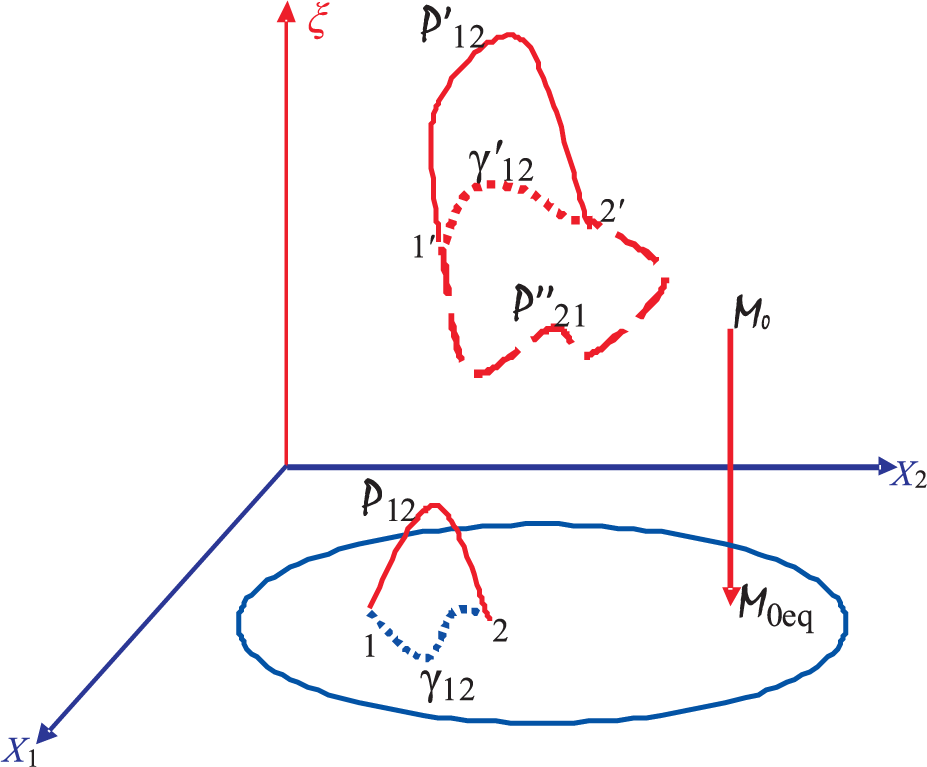
  • 18It must be remarked that a (thermodynamic) cyclic process is not possible for an isolated system. Such a system can only undergo a spontaneous process 00eq in Figure 2, which represents the spontaneous relaxation going on within Σ0 as the system tries to approach equilibrium. For Σ0 to return to 0 will violate the second law.
  • 19If there is a repeating ANEQS for which its entropy has the repeating property S(Z(t + τC), t + τC) = S(Z(t), t) for a particular cycle time τC (of course, Z(t + τC) = Z(t)), one can construct a cyclic process with this state as the starting and the repeating state. It is clear that Equation (3) will also hold for such a cycle. We will not consider such a cyclic process here as it is a cycle only of a fixed cycle time.
  • 20Here, we follow the ideas of Maxwell and Thomson, embodied in the second law of thermodynamics, that when a constraint is lifted, an isolated macroscopic system will evolve toward a state of higher entropy [55,56].
  • 21We assume that k e k ( t ) 0. The additivity of energy, a mechanical quantity, is therefore a consequence of a mechanical independence of subsystems.
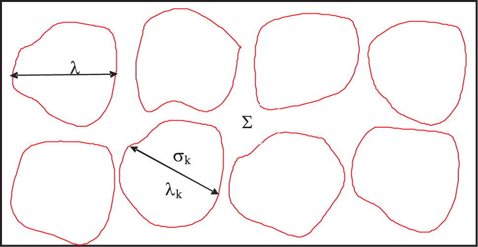
  • 22We assume that there is a single correlation length. If there are several correlation lengths, we take the longest of all for the discussion.
  • 23We say that the two subsystems are thermodynamically independent as this independence is needed for S, which is a thermodynamic concept.
  • 24We find it useful to think of S ˜ ( Z ˜ ( t ) ) as a function not only of the observables but also of internal variables in this section, even though the latter are not independent, so that we can later expand S ˜ ( Z ˜ ( t ) ) around Z0(t).
  • 25Compare GX(t) with the concept of generalized available energy [5].
  • 26The constraint is to disallow ordered configurations responsible for crystallization.
  • 27It should be stressed that as it has not been possible to get to absolute zero, some extrapolation is always needed to determine Sexpt(0).
  • 28It should be recalled that Boltzmann needed to assume molecular chaos to derive the second law; microscopic Newtonian dynamics of individual particles alone is not sufficient for the derivation; see for example [52] for justification, where it has been shown that microscopic Newtonian dynamics cannot bring about equilibration in an isolated body that is not initially in equilibrium. However, not everyone believes that the second law cannot be derived from Newtonian mechanics.
  • 29The sets m and p should not be confused with the angular and linear momenta in the previous section.
  • 30The entropy formulation in Equation (52) can include pα = 0 without any harm, even though it is preferable to not include it as the definition of the set m0(Z0) and the number W0(Z0) only includes microstates with non-zero probabilities.
  • 31A thermodynamically significant number a is exponential (~ eαN) in the number of particles N with α > 0. This ensures that 1 N as N → ∞. One can also consider the limiting form of a as α → 0 from above.
  • 32The adiabatic approximation (very slow variation of parameters in time) in mechanics [90] should not be confused with thermodynamic adiabatic approximation for which deQ = 0.
  • 33The partition function Z should not be confused with the state variable Z.
  • 34The enrgy E contains only the kinetic energy of translation, which determines the temperature. However, the kinetic energy is of no concern in the follwing for studying the configurational entropy sc.
  • 35Observe that we do not consider S/N or S/Nf as these quantities are ambiguous because the denomenators may depend on the state but also because they vanish in the limit.
  • 36Other derivations in the literature such as the derivation by Hatsopoulos and Gyftopoulos [99] or Beretta [100] assume equations of motion to obtain the statistical entropy.

References and Notes

  1. Clausius, R. The Mechanical Theory of Heat; Macmillan & Co.: London, UK, 1879. [Google Scholar]
  2. De Donder, Th.; van Rysselberghe, P. Thermodynamic Theory of Affinity; Stanford University: Stanford, CA, USA, 1936. [Google Scholar]
  3. De Groot, S.R.; Mazur, P. Non-Equilibrium Thermodynamics, 1st ed; Dover: New York, NY, USA, 1984. [Google Scholar]
  4. Landau, L.D.; Lifshitz, E.M. Statistical Physics, 3rd ed; Pergamon Press: Oxford, UK, 1986; Volume 1. [Google Scholar]
  5. Gyftopoulos, E.P.; Beretta, G.P. Thermodynamics Foundations and Application; Macmillan Publishing Company: New York, NY, USA, 1991. [Google Scholar]
  6. Kondepudi, D.; Prigogine, I. Modern Thermodynamics; John Wiley and Sons: West Sussex, UK, 1998. [Google Scholar]
  7. Öttinger, H.C. Beyond Equilibrium Thermodynamics; Wiley-Interscience: Hoboken, NJ, USA, 2005. [Google Scholar]
  8. Mueller, I.; Ruggeri, T. Rational Extended Thermodynamics, 2nd ed; Springer-Verlag: New York, NY, USA, 1998. [Google Scholar]
  9. Lebon, G.; Joue, D.; Casas-Vásgues, J. Understanding Non-equilibrium Thermodynamics; Springer-Verlag: Berlin/Heidelberg, Germany, 2008. [Google Scholar]
  10. Gibbs, J.W. Elementary Principles in Statistical Mechanics; Yale University Press: New Haven, CT, USA, 1960. [Google Scholar]
  11. Tolman, R.C. The Principles of Statistical Mechanics; Oxford University: London, UK, 1959. [Google Scholar]
  12. Rice, S.A.; Gray, P. The Statistical Mechanics of Simple Liquids; Interscience Publishers: New York, NY, USA, 1965. [Google Scholar]
  13. Keizer, J. Statistical Thermodynamics of Nonequilibrium Processes; Springer-Verlag: New York, NY, USA, 1987. [Google Scholar]
  14. Campisi, M.; Hänggi, P.; Talkner, P. Quantum fluctuation relations: Foundations and applications. Rev. Mod. Phys. 2011, 83, 771–791. [Google Scholar]
  15. Siefert, U. Stochastic thermodynamics: principles and perspectives. Eur. Phys. J. B. 2008, 64, 423–431. [Google Scholar]
  16. Gawedzki, K. Fluctuation Relations in Stochastic Thermodynamics 2013, arXiv, 1308.1518v1.
  17. Landau, L.D.; Lifshitz, E.M. Quantum Mechanics, 3rd ed; Pergamon Press: Oxford, UK, 1977. [Google Scholar]
  18. Von Neumann, J. Mathematical Foundations of Quantum Mechanics; Princeton University Press: Princeton, NJ, USA, 1996. [Google Scholar]
  19. Partovi, M.H. Entropic Formulation of Uncertainty for Quantum Measurements. Phys. Rev. Lett. 1983, 50, 1883–1885. [Google Scholar]
  20. Bender, C.M.; Brody, D.C.; Meister, B.K. Quantum mechanical Carnot engine. J. Phys. A. 2000, 33, 4427–4436. [Google Scholar]
  21. Unusual quantum states: Non–locality, entropy, Maxwell’s demon and fractals. Proc. R. Soc. A. 2005, 461, 733–753.
  22. Scully, M.O.; Zubairy, M.S.; Agarwal, G.S.; Walther, H. Extracting Work from a Single Heat Bath via Vanishing Quantum Coherence. Science 2003, 299, 862–864. [Google Scholar]
  23. Beckenstein, J.D. Black Holes and Entropy. Phys. Rev. D. 1973, 7, 2333–2346. [Google Scholar]
  24. Beckenstein, J.D. Statistical black-hole thermodynamics, ibid. Phys. Rev. D 1975, 12, 3077–3085. [Google Scholar]
  25. Schumacker, B. Quantum coding. Phys. Rev. A. 1995, 51, 2738–2747. [Google Scholar]
  26. Bennet, C.H. The Thermodynamics of Computation—A Review. Int. J. Theor. Phys. 1982, 21, 905–940. [Google Scholar]
  27. Bennet, C.H. Quantum information. Phys. Scr. 1998, T76, 210–217. [Google Scholar]
  28. Wiener, N. Cybernetics; MIT Press: Cambridge, UK, 1948. [Google Scholar]
  29. Shannon, C.E. A Mathematical Theory of Communication. Bell Syst. Tech. J. 1948, 27, 379–423. [Google Scholar]
  30. Balian, R. Entropy, a Protean Concept. Poincaré Semianr 2003, 2, 119–145. [Google Scholar]
  31. Lieb, E.H.; Yngvason, J. The physics and mathematics of the second law of thermodynamics. Phys. Rep. 1999, 310, 1–96. [Google Scholar]
  32. Lieb, E.H.; Yngvason, J. The entropy concept for non-equilibrium states 2013, arXiv, 1305.3912.
  33. Gyftopoulos, E.P.; Çubukçu, E. Entropy: Thermodynamic definition and quantum expression. Phys. Rev. E. 1997, 55, 3851–3858. [Google Scholar]
  34. Beretta, G.P.; Zanchini, E. A definition of thermodynamic entropy valid for non-equilibrium states and few-particle systems 2014, arXiv, 1411.5395.
  35. Gujrati, P.D. Non-equilibrium Thermodynamics: Structural Relaxation, Fictive temperature and Tool-Narayanaswamy phenomenology in Glasses. Phys. Rev. E. 2010, 81, 051130. [Google Scholar]
  36. Gujrati, P.D. Nonequilibrium thermodynamics. II. Application to inhomogeneous systems. Phys. Rev. E. 2012, 85, 041128. [Google Scholar]
  37. Gujrati, P.D.; Aung, P.P. Nonequilibrium thermodynamics. III. Generalization of Maxwell, Clausius-Clapeyron, and response-function relations, and the Prigogine-Defay ratio for systems in internal equilibrium. Phys. Rev. E. 2012, 85, 041129. [Google Scholar]
  38. Gujrati, P.D. Generalized Non-equilibrium Heat and Work and the Fate of the Clausius Inequality 2011, arXiv, 1105.5549.
  39. Gujrati, P.D. Nonequilibrium Thermodynamics. Symmetric and Unique Formulation of the First Law, Statistical Definition of Heat and Work, Adiabatic Theorem and the Fate of the Clausius Inequality: A Microscopic View 2012, arXiv, 1206.0702. [Google Scholar]
  40. Lieb, E.H.; Lebowitz, J.L. The constitution of matter: Existence of thermodynamics for systems composed of electrons and nuclei. Adv. Math. 1972, 9, 316–398. [Google Scholar]
  41. Gallavotti, G. Entropy production in nonequilibrium thermodynamics: A review 2004, arXiv, cond-mat/0312657v2.
  42. Ruelle, D. Positivity of entropy production in nonequilibrium statistical mechanics. J. Stat. Phys. 1996, 85, 1–25. [Google Scholar]
  43. Ruelle, D. Extending the definition of entropy to nonequilibrium steady states. Proc. Natl. Acad. Sci. 2003, 85, 3054–3058. [Google Scholar]
  44. Oono, Y.; Paniconi, M. Steady state thermodynamics. Prog. Theor. Phys. 1998, 30, 29–44. [Google Scholar]
  45. Maugin, G.A. The Thermomechanics of Nonlinear Irreversible Behaviors: An Introduction; World Scientific: Singapore, Singapore, 1999. [Google Scholar]
  46. Beretta, G.P.; Zanchini, E. Rigorous and General Definition of Thermodynamic Entropy. In Thermodynamics; Tadashi, M., Ed.; InTech: Rijeka, Croatia, 2011; pp. 23–50. [Google Scholar]
  47. Canessa, E. Oscillating Entropy 2013, arXiv, 1307.6681.
  48. Sasa, S. Possible extended forms of thermodynamic entropy 2013, arXiv, 1309.7131.
  49. Beretta, G.P.; Zanchini, E. Removing Heat and Conceptual Loops from the Definition of Entropy. Int. J. Thermodyn. 2010, 12, 67–76. [Google Scholar]
  50. Feynman, R.P. The Feynman Lectures on Physics; Addison-Wesley: Boston, MA, USA, 1963; Volume 1. [Google Scholar]
  51. Zanchini, E.; Beretta, G.P. Recent Progress in the Definition of Thermodynamic Entropy. Entropy 2014, 16, 1547–1570. [Google Scholar]
  52. Gujrati, P.D. Loss of Temporal Homogeneity and Symmetry in Statistical Systems: Deterministic Versus Stochastic Dynamics. Symmetry 2010, 2, 1201–1249. [Google Scholar]
  53. Bishop, R.C. Nonequilibrium Statistical Mechanics Brussels-Austin. Style. Stud. Hist. Philos. Mod. Phys. 2004, 35, 1–30. [Google Scholar]
  54. Lavis, D.A. Boltzmann, Gibbs, and the Concept of Equilibrium. Philos. Sci. 2008, 75, 682–696. [Google Scholar]
  55. Lebowitz, J. Statistical mechanics: A selective review of two central issues. Rev. Mod. Phys. 1999, 71, S346–S357. [Google Scholar]
  56. Goldstein, S.; Lebowitz, J.L. On the (Boltzmann) Entropy of Nonequilibrium Systems 2003, arXiv, cond-mat/0304251.
  57. Palmer, R.G. Broken ergodicity. Adv. Phys. 1982, 31, 669–735. [Google Scholar]
  58. Gujrati, P.D. Energy gap Model of Glass Formers: Lessons Learned from Polymers. In Modeling and Sinulation in Polymers; Gujrati, P.D., Leonov, A.I., Eds.; Wiley-VCH: Weinheim, Germany, 2010; pp. 433–495. [Google Scholar]
  59. Gujrati, P.D. General theory of statistical fluctuations with applications to metastable states, Nernst points, and compressible multi-component mixtures. Recent Res. Devel. Chem. Phys. 2003, 4, 243–275. [Google Scholar]
  60. Planck, M. Über das Gesetz der Energieverteilung im Normalspektrum. Ann. Phys. 1901, 4, 553–563. [Google Scholar]
  61. Boltzmann, L. Über die Beziehung zwischen dem zweiten Hauptsatze der mechanischen Wärmtheorie und der Wahrscheinlichkeitscrechnung respektive den Sätzen über das Wärmegleichgewicht. Wien Ber 1877, 76, 373–435. [Google Scholar]
  62. Boltzman, L. Lectures on Gas Theory; University of California Press: Berkeley, CA, USA, 1964; pp. 55–62. [Google Scholar]
  63. The number of combinations in Equation (35) on p. 56 in Boltzmann [62] is denoted by Z, but it is not the number of microstates. The two become the same only when Z is maximized as discussed on p. 58
  64. Jaynes, E.T. Gibbs vs. Boltzmann Entropies. Am. J. Phys. 1965, 33, 391–398. [Google Scholar]
  65. Cohen, E.G.D. Einstein and Boltzmann: Determinism and Probability or The Virial Expansion Revisited 2013, arXiv, 1302.2084.
  66. Pokrovskii, V.N. A Derivation of the Main Relations of Nonequilibrioum Thermodynamics. ISRN Thermodyn 2013. [Google Scholar] [CrossRef]
  67. Landau, L.D.; Lifshitz, E.M. Fluid Mechanics; Pergamon Press: Oxford, UK, 1982. [Google Scholar]
  68. Edwards, S.F.; Oakeshott, R.S.B. Theory of Powders. Physica 1989, 157A, 1080–1090. [Google Scholar]
  69. Bouchbinder, E.; Langer, J.S. Nonequilibrium thermodynamics of driven amorphous materials. I. Internal degrees of freedom and volume deformation. Phys. Rev. E. 2009, 80, 031131. [Google Scholar]
  70. Gutzow, I.; Schmelzer, J. The Vitreous State Thermodynamics, Structure, Rheology and Crystallization; Springer-Verlag: Berlin/Heidelberg, Germany, 1995. [Google Scholar]
  71. Nemilov, S.V. Thermodynamic and Kinetic Aspects of the Vitreous State; CRC Press: Boca Raton, FL, USA, 1995. [Google Scholar]
  72. Gujrati, P.D. Where is the residual entropy of a glass hiding? 2009, arXiv, 0908.1075.
  73. Jäckle, J. On the glass transition and the residual entropy of glasses. Philos. Mag. B. 1981, 44, 533–545. [Google Scholar]
  74. Jäckle, J. Residual entropy in glasses and spin glasses. Physica B 1984, 127, 79–86. [Google Scholar]
  75. Gibson, G.E.; Giauque, W.F. The third law of thermodynamics. evidence from the specific heats of glycerol that the entropy of a glass exceeds that of a crystal at the absolute zero. J. Am. Chem. Soc. 1923, 45, 93–104. [Google Scholar]
  76. Giauque, W.E.F.; Ashley, M. Molecular Rotation in Ice at 10K. Free Energy of Formation and Entropy of Water. Phys. Rev. 1933, 43, 81–82. [Google Scholar]
  77. Pauling, L. The Structure and Entropy of Ice and of Other Crystals with Some Randomness of Atomic Arrangement. J. Am. Chem. Soc. 1935, 57, 2680–2684. [Google Scholar]
  78. Bestul, A.B.; Chang, S.S. Limits on Calorimetric Residual Entropies of Glasses. J. Chem. Phys. 1965, 43, 4532–4533. [Google Scholar]
  79. Nagle, J.F. Lattice Statistics of Hydrogen Bonded Crystals. I. The Residual Entropy of Ice. J. Math. Phys. 1966, 7, 1484–1491. [Google Scholar]
  80. Bowles, R.K.; Speedy, R.J. The vapour pressure of glassy crystals of dimers. Mole. Phys. 1996, 87, 1349–1361. [Google Scholar]
  81. Isakov, S.V.; Raman, K.S.; Moessner, R.; Sondhi, S.L. Magnetization curve of spin ice in a [111] magnetic field. Phys. Rev. B. 2004, 70, 104418. [Google Scholar]
  82. Berg, B.A.; Muguruma, C.; Okamoto, Y. Residual entropy of ordinary ice from multicanonical simulations. Phys. Rev. B. 2007, 75, 092202. [Google Scholar]
  83. Gujrati, P.D. Poincare Recurrence, Zermelo’s Second Law Paradox, and Probabilistic Origin in Statistical Mechanics 2008, arXiv, 0803.0983.
  84. Searles, D.; Evans, D. Fluctuations relations for nonequilibrium systems. Aust. J. Chem. 2004, 57, 1119–1123. [Google Scholar]
  85. Jaynes, E.T. Information Theory and Statistical Mechanics. Phys. Rev. 1957, 106, 620–630. [Google Scholar]
  86. Jaynes, E.T. Information Theory and Statistical Mechanics. II, ibid. Phys. Rev. 1957, 108, 171–190. [Google Scholar]
  87. Jaynes, E.T. Prior Probabilities. IEEE Trans. Syst. Sci. Cybern. 1968, 4, 227–241. [Google Scholar]
  88. Jaynes, E.T. Probability Theory: The logic of Science; Cambridge University Press: New York, NY, USA, 2003. [Google Scholar]
  89. Bagci, G.B.; Oikonomou, T.; Tirnakli, U. Comment on “Essential discreteness in generalized thermostatistics with non-logarithmic entropy” by S. Abe 2010, arXiv, 1006.1284v2.
  90. Landau, L.D.; Lifshitz, E.M. Mechanics, 3rd ed; Pergamon Press: Oxford, UK, 1976. [Google Scholar]
  91. Holian, B.L. Entropy evolution as a guide for replacing the Liouville equation. Phys. Rev. A. 1986, 34, 4238–4245. [Google Scholar]
  92. Holian, B.L.; Hoover, W.G.; Posch, H.A. Resolution of Loschmidt’s paradox: The origin of irreversible behavior in reversible atomistic dynamics. Phys. Rev. Lett. 1987, 59, 10–13. [Google Scholar]
  93. Ramshaw, J.D. Remarks on entropy and irreversibility in non-hamiltonian systems. Phys. Lett. A. 1986, 116, 110–114. [Google Scholar]
  94. Hoover, W.G. Liouville’s theorems, Gibbs’ entropy, and multifractal distributions for nonequilibrium steady states. J. Chem. Phys. 1998, 109, 4164–4170. [Google Scholar]
  95. Semerianov, F.; Gujrati, P.D. Configurational entropy and its crisis in metastable states: Ideal glass transition in a dimer model as a paragidm of a molecular glass. Phys. Rev. E. 2005. [Google Scholar] [CrossRef]
  96. Tonks, L. The Complete Equation of State of One, Two and Three-Dimensional Gases of Hard Elastic Spheres. Phys. Rev. 1936, 50, 955–963. [Google Scholar]
  97. Thompson, C. Mathematical Statistical Mechanics; Princeton University Press: Princeton, NJ, USA, 1972. [Google Scholar]
  98. Gujrati, P.D. A binary mixture of monodisperse polymers of fixed architectures, and the critical and the theta states. J. Chem. Phys. 1998, 108, 5104–5121. [Google Scholar]
  99. Hatsopoulos, G.N.; Gyftopoulos, E.P. A unified quantum theory of mechanics and thermodynamics, Part I. Postulates Found. Phys. 1976, 6, 15–31. [Google Scholar]
  100. Beretta, G.P. Quantum Thermodynamics of Non-Equilibrium. Onsager Reciprocity and Dispersion-Dissipation Relations. Found. Phys. 1987, 17, 365–381. [Google Scholar]
Figure 1. Schematic representation a body representing (a) an isolated system Σ0 or (b) the interacting system Σ in a medium Σ ˜; the two have their boundaries disjoint and together form the isolated system Σ0. The medium is extremely large compared to the system Σ, so its fields T ˜ ( t ), P ˜ ( t ), ⋯ etc. are almost the same as T0, P0, ⋯ of Σ0 so we will not make any distinction between them. If and only if the body is in internal equilibrium, see text, we can define its fields T(t), P(t), ⋯ etc. For the body Σ in (b), these fields need not be equal to the corresponding fields T0, P0, ⋯ of the medium Σ ˜, unless Σ and Σ ˜ are in equilibrium. The changes diX and deX during any process (reversible or irreversible) in any extensive quantity associated with a body give the net change dXdiX + deX. Here, diX represents the (internal) change (suffix i) in X occurring within the body and deX represents the exchange (suffix e) of X with the medium as shown by the double arrow; the latter is absent for the body in (a). Away from equilibrium, there will be viscous dissipation within the body, which results in the irreversible entropy generation diS > 0 within the body.
Entropy 17 00710f1
Figure 2. The equilibrium macrostates correspond to ξ = 0 and lie in the enclosed region of the X1X2 plane shown schematically by the closed curve in solid blue. The enclosed region represents the equilibrium region. The two equilibrium macrostates 1eq and 2eq for an interacting system are indicated by 1 and 2 in this plane. A possible nonequilibrium process between 1 and 2 is shown by P 12 as a solid red curve that leaves the equilibrium region along ξ ≠ 0 from 1 and then comes back to 2. The path γ12 lies in the equilibrium region and represents one of many possible equilibrium processes connecting 1 with 2. The nonequilibrium macrostate 0 of an isolated system Σ0 approaches equilibrium along the solid red arrow at fixed X = X0 and turns into the macrostate 0eq within the equilibrium region. The macrostates 1′ and 2′ represent two nonequilibrium states in internal equilibrium with ξ ≠ 0 with processes P 12 and P 21 between them. All the states with ξ ≠ 0 along the path γ 12 but not necessarily along P 12 and P 21 between 1′ and 2′ represent states in internal equilibrium.
Entropy 17 00710f2
Figure 3. An inhomogeneous body Σ and its various subsystems σk, k = 1, 2, 3, … As the kth subsystem is of size λk as explained in the text, the subsystems are uncorrelated and can be treated as quasi-independent.
Entropy 17 00710f3
Figure 4. Schematic behavior of the entropy of the constrained equilibrated liquid, i.e., the supercooled liquid (solid curve) and a possible glass (dotted curve) during vitrification. The transition region between T0g and T0G has been exaggerated to highlight the point that the glass transition is not a sharp point. For all temperatures T0 < T0g, any nonequilibrium state undergoes isothermal structural relaxation in time towards the supercooled liquid. The entropy of the supercooled liquid is shown to extrapolate to zero per our assumption, but that of the glass to a non-zero value SR at absolute zero.
Entropy 17 00710f4

