Analysis of the Magnetocaloric Effect in Heusler Alloys: Study of Ni50CoMn36Sn13 by Calorimetric Techniques

Abstract

Direct determinations of the isothermal entropy increment, −ΔS_T, in the Heusler alloy Ni₅₀CoMn₃₆Sn₁₃ on demagnetization gave positive values, corresponding to a normal magnetocaloric effect. These values contradict the results derived from heat-capacity measurements and also previous results obtained from magnetization measurements, which indicated an inverse magnetocaloric effect, but showing different values depending on the technique employed. The puzzle is solved, and the apparent incompatibilities are quantitatively explained considering the hysteresis, the width of the martensitic transition and the detailed protocol followed to obtain each datum. The results show that these factors should be analyzed in detail when dealing with Heusler alloys.

1. Introduction

The discovery in 1997 of the so-called “giant magnetocaloric effect” (GMCE) in Gd₅Si₂Ge₂ [1] triggered a true explosion of the research effort, not only on stronger, efficient and less expensive materials, but also on magnetic refrigeration systems, which eventually could replace the conventional refrigeration machines based on the compression-expansion cycles of a fluid. Today, the most promising materials can be grouped into a few families of compounds, each one belonging to a common crystal structure and including chemically similar elements in each group. Among them, we can mention the compounds derived from MnAs [2,3], MnFeP_1−xAs_x [4] and LaFe_13−xSi_x [5]. In a conventional ferromagnetic or paramagnetic material, the maximum entropy reduction on an applied magnetic field is k_B ln(2S + 1) per magnetic atom. This corresponds to the change from a fully disordered state with random orientation of spins at zero field to a fully ordered state with spins aligned under a strong magnetic field. The GMCE compounds have a higher entropy reduction than conventional materials for a moderate field, because they often undergo a first-order structural transition from a low magnetization phase, which we call non-magnetic and is usually paramagnetic, to a ferromagnetic one. This transition occurs spontaneously at some temperature and can be induced by a moderate external magnetic field above this temperature. However, the magnetization of the ferromagnetic phase is not near saturation at the practical temperatures for room temperature refrigeration, so that the maximum magnetic entropy change that can be induced is below the theoretical limit.

The entropy reduction is not necessarily limited to the magnetic entropy. This limit can be overcome, because the total entropy is a sum of three contributions:

$$S=S_m+S_e+S_{ph}$$

(1)

where S_m is the magnetic contribution, coming from the population of the unpaired spin states, essentially due to the inner electrons, S_e is the electronic contribution, due to the conduction electrons, and S_ph is the phonon contribution, due to the atomic vibrations in the lattice. In a first-order transition, the entropy is discontinuous, and the more stable phase is the one with the lowest free energy for a given temperature and field. An external field reduces the free energy of the magnetic phase by −MB, which allows increasing its stability at temperatures at which the stable phase is non-magnetic in the absence of the field. The total entropy change produced by a field change at constant temperature is denoted ΔS_T. It is quite often and wrongly called “magnetic entropy change”; but actually, all of the three terms in Equation (1) contribute, and sometimes, ΔS_m is not even the most relevant term. On increasing the external field in a paramagnetic substance, ΔS_m < 0, because the magnetic dipoles tend to order orienting towards the field direction, but ΔS_e and ΔS_ph can be positive or negative.

Compounds exhibiting an inverse magnetocaloric effect [6] (IMCE) behave differently upon a field change, because the ferromagnetic phase occurs above the zero field transition temperature, T_t, and consequently, the total entropy is higher than that of the non-magnetic phase. Below T_t, an external magnetic field applied isothermally can convert the non-magnetic phase into a magnetic one, with a positive entropy increment that corresponds to ΔS_T > 0, with ΔS_m ≤ 0 and ΔS_e + ΔS_ph > 0. Both, the phonon and the electronic entropy changes can give important contributions to ΔS_T. Strong magnetostructural correlations have been reported in these Heusler alloys [7], and sharp increases in the electrical conductivity have been found in the transition to the ferromagnetic austenite [8], indicating a high increase in the density of electronic states at the Fermi level. A study case with a main electronic entropy term is Mn₃GaC. In this compound, the low temperature phase, with no neat spontaneous magnetization, is magnetically ordered. ΔS_m at the transition is very small, and consequently, ΔS_T is nearly independent of the field if it reaches a threshold value [9], which, in turn, increases when the temperature decreases from T_t. The consequence is the very interesting feature that, near T_t, even a low magnetic field can produce the full entropy change, while for typical or, even, for GMCE compounds, a strong magnetic field is necessary to produce a significant entropy change.

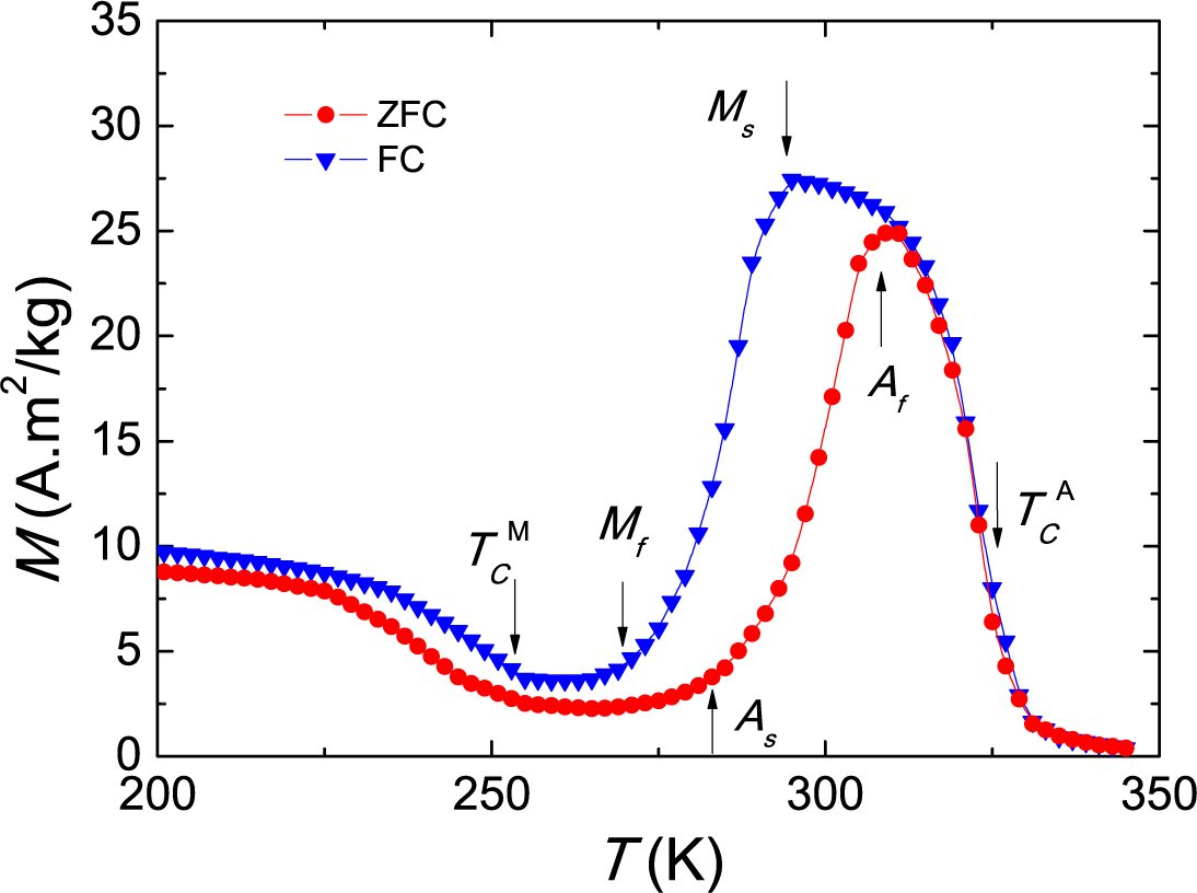
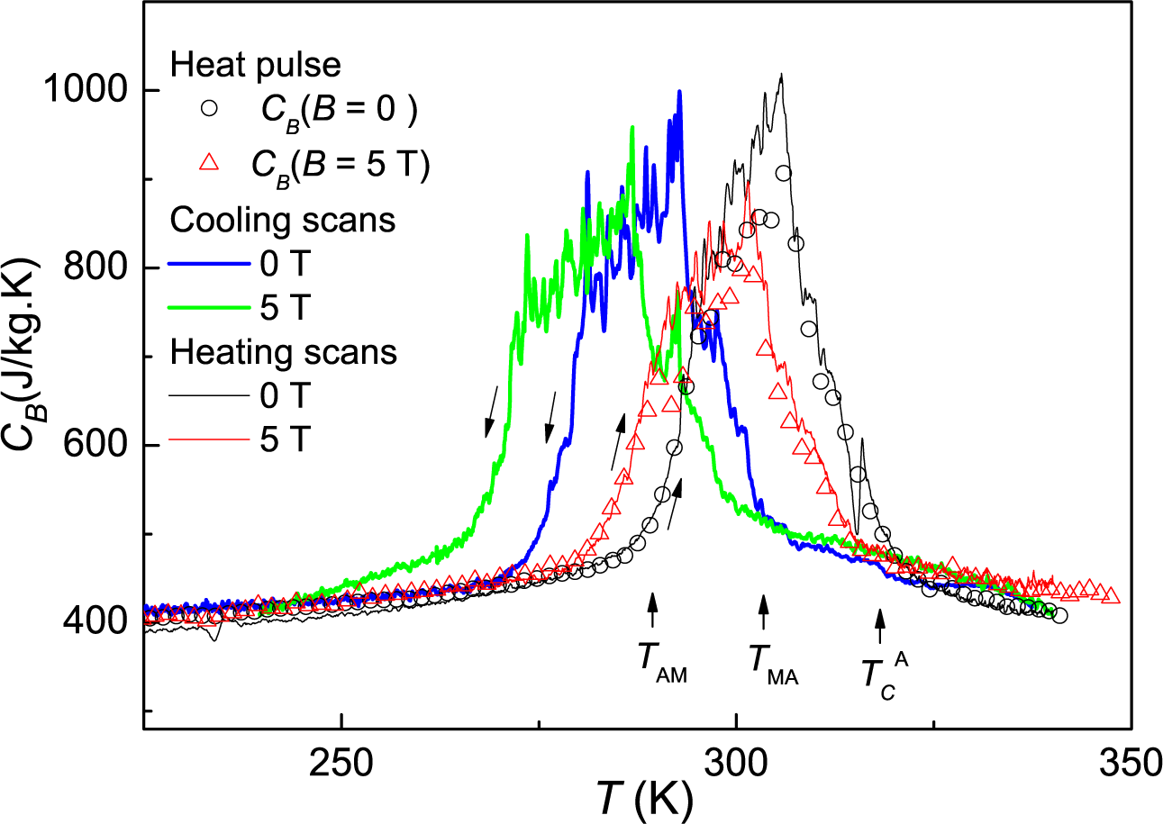
The Heusler alloys, Ni₅₀Co_yMn_25+z−yM_25−z, with M = Sn, In, Sb, offer the possibility of having a similar behavior to Mn₃GaC, but near room temperature and with a stronger entropy change. They are derived from the stoichiometric Ni₂MnGa and have been widely studied, because of their property of shape memory controlled by the application of magnetic field. On heating, these compounds undergo a first-order transition from a low symmetry phase called “martensite” (M) to another cubic phase called “austenite” (A) at a temperature T_MA. This transition has a large latent heat and, consequently, a strong entropy increment, typically near 25–30 J/kg·K. On the other hand, the transition is usually broad and has a wide thermal hysteresis, with the reverse transition at T_AM < T_MA, so that four temperatures are given as characteristic parameters: the M to A starting transition temperature on heating, A_s, the finishing temperature of this transition, A_f, the A to M starting transition temperature, M_s, and its finishing temperature, M_f, with M_f < T_AM < M_s and A_s < T_MA < A_f. In addition to this, the M phase has a lower magnetization than the A phase, as seen in Figure 1. The respective Curie points are denoted as $T_C^A$ and $T_C^M$. For a general picture of the dependence of these temperatures with the composition, we refer to the compositional phase diagram given in [6,10]. While M_s and M_f decrease and $T_C^M$ increases strongly on decreasing the Sn content, $T_C^A$ remains nearly constant. We chose the value z = 12 in order to get $T_C^M<M_f$. On the other hand, the addition of a small amount of Co increases $T_C^A$ and decreases M_s and M_f [11,12]. The parameter y = 1 has been chosen with the aim of having $T_C^M<M_f<M_s<T_C^A$ (Figure 1). This would allow one to have a strong IMCE for the transition between paramagnetic martensite and ferromagnetic austenite when a field is applied to the martensite phase between $T_C^M$ and A_s.

Actually, a strong IMCE has been reported in several compounds, but the various results do not agree and are even contradictory, depending on the technique used to determine ΔS_T and on the experimental protocol. These protocols, taken as the sequence of fields and temperatures applied to the sample, are not usually reported in detail. For instance, in Ni₄₃Mn₄₆Sn₁₁, [13] reports, for a field change from 2 T to 5 T, a maximum ΔS_T,max = 2.6 J/kg·K at 184 K from heat capacity data, but ΔS_T,max = 46.9 J/kg·K at 190 K from isothermal magnetization computed via the Maxwell relation. For Ni₅₀CoMn₃₆Sn₁₃, ΔS_T,max ≈ 12 J/kg·K from magnetization at constant fields on heating and on cooling, for a field change from 0 to 2 T [14], but the Clausius–Clapeyron equation predicts ΔS_T,max ≈ 26 J/kg·K. Similar discrepancies between the results obtained from heat capacity measurements and via the Maxwell relation have been reported for Ni₄₆Cu₄Mn₃₈Sn₁₂ and Ni₅₀CoMn₃₄In₁₅ [15]. The direct measurements of the adiabatic temperature increment, ΔT_S, gave no inverse MCE on cooling and obtained inconsistent values with those on heating [14]. The importance of the hysteresis and the influence of the measurement protocols have been analyzed on this type of compound [16]. For the close composition Ni₄₈Co₂Mn₃₈Sn₁₂, [12] gives ΔS_T,max = 37.1 J/kg·K from isothermal magnetization, for a field change of 5 T.

The aim of the present work is to compare the existing results for ΔS_T and ΔT_S with new directly measured values and results deduced from heat capacity at constant fields, C_B, on the chosen compound, Ni₅₀CoMn₃₆Sn₁₃. The experimental protocols are carefully considered in all cases, and the different results are explained considering the characteristics of the sample and the details of the protocols used in the determinations.

2. Measurement Protocols and Experimental Effects

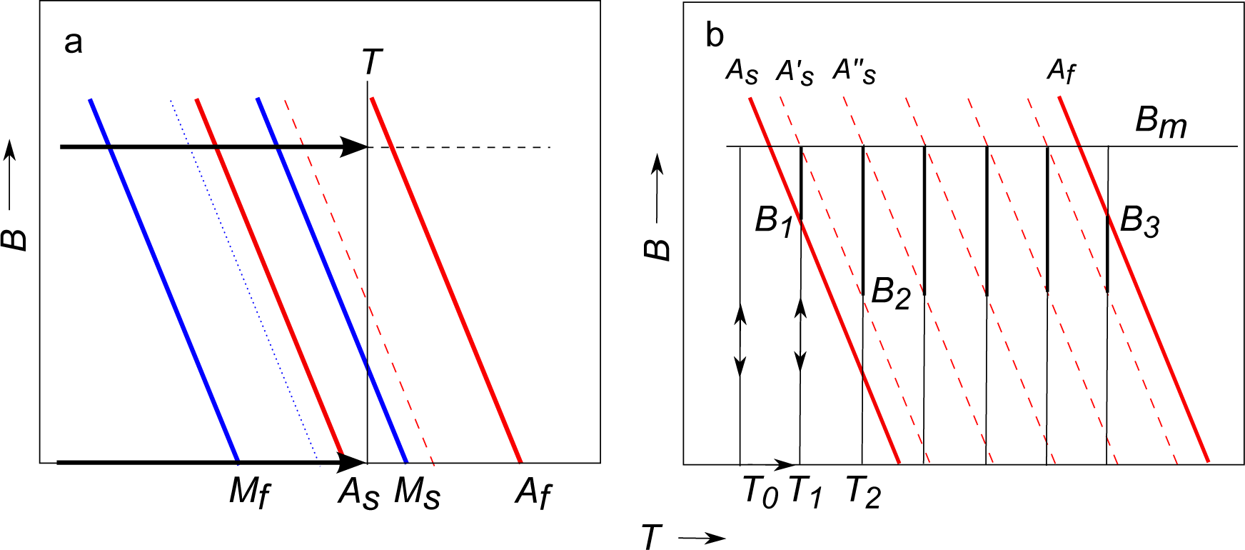
A scheme of a B − T phase diagram near the martensitic transition region is depicted in Figure 2a. The continuous red lines indicate the set of points A_s and A_f for the M to A conversion and the blue lines the set of points M_s and M_f for the transition from A to M. The specific entropy of the sample at a given temperature, T, and field, B, is S(T, B, x) = xS_A(T, B) + (1 − x)S_M(T, B), being S_A, S_M the specific entropies of the austenite and martensite phases and 0 ≤ x ≤ 1 the fraction of austenite. Due to the hysteresis, x and the total entropy depend not only on T and B, but also on the path followed by the state point to reach a particular point in the B − T diagram. Therefore, the true isothermal entropy difference, ΔS_T, between two states at the same T and different B depends on the protocol followed by the sample to reach both states.

The sample is composed of many grains and domains, each one having slightly different compositions, microstructures or sizes, which, in turn, cause different transition temperatures, T_MA and T_AM, since they are very sensitive to the proportion Mn/Sn and their site occupancy. On the other hand, the specific latent heat for every grain is practically constant, which implies that the transition lines are nearly straight lines with the same slope for all grains, due to the Clausius–Clapeyron equation. This means that the fraction x depends only on T and B for every state reached in any process involving phase conversion in only one direction, M to A or A to M. The curves of constant x are parallel straight lines, as indicated by the red dashed lines in Figure 2 for heating or magnetization processes. Similarly, on cooling or demagnetization processes, the constant x curves are represented by the blue lines. The experimental phase diagram of a small piece of our compound was given in Figure 6 of [14]. For the present sample, the width of the transition bands is broader and the transition temperatures slightly higher.

We will consider several processes, frequently used in experiments, represented by the evolution of a state point in the phase diagram. We will discuss the expected behavior for each protocol, which is applicable to compounds having a martensitic transition. This general analysis will be applied to our experimental results on Ni₅₀CoMn₃₆Sn₁₃, comparing direct measurements of ΔS_T with values deduced from heat capacities on heating and cooling and results from isofield magnetization data.

2.1. Protocol a: Isofield Heating

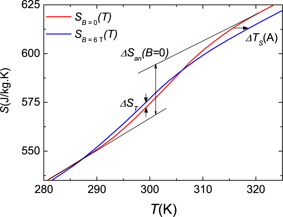
The simplest protocol is heating at a constant field starting from a low temperature. This is used in heat capacity determinations, as is indicated by the arrows at zero and B fields in Figure 2a. The integration of C_B/T gives the entropy increment with respect to some arbitrary temperature of reference, T₀. Knowing the entropy difference for different fields at T₀ from direct measurements, as seen below in protocol c, one can compute the entropies at any temperature and field and calculate the difference. The values for ΔS_T are obtained as the entropy difference between the sample heated at a field B and the sample heated at zero field. This corresponds to the isothermal entropy increment upon increasing the field from zero to B for the sample previously heated up to T at B = 0.

Leaving apart experimental errors, this procedure introduces other small errors when going through first-order transitions due to the irreversibility of the hysteretic processes. There is an irreversible entropy production at the transition, and the supplied heat is lower than the product of the entropy increment times the temperature. The irreversible entropy is proportional to the thermal hysteresis δS_i/ΔS_T = (T_MA − T_AM)/(T_MA + T_AM), as given in [17], being in our compound around 0.025, considering the values reported below in

Table 1. Main parameters for the martensitic transition of Ni₅₀CoMn₃₆Sn₁₃ deduced from the heat capacity at various fields. T_AM and T_MA, martensitic transition temperatures. ΔH_an and ΔS_an, enthalpy and entropy of transition.

B(T)	TAM(K)	TMA(K)	|ΔHan|(J/g)	|ΔSan|(J/kg·K)	Method
0	–	302.9	9.7(5)	32(2)	Heat pulse
0	–	303.3	12.0(7)	39(2)	Heating
0	289.3	–	11.2(7)	38(2)	Cooling
1	–	302.3	9.4(6)	31(2)	Heat pulse
1	288.7	–	12.2(7)	42(3)	Cooling
2	–	301.1	9.3(6)	31(2)	Heat pulse
3	–	299.6	9.0(5)	30(2)	Heat pulse
3	–	300.3	10.2(6)	34(2)	Heating
3	286.2	–	12.6(8)	44(3)	Cooling
5	–	297.3	8.9(5)	29(2)	Heat pulse
5	–	297.9	9.9(6)	33(2)	Heating
5	282.4	–	12.6(8)	44(3)	Cooling

. Therefore, this is a small correction in the present case, where huge differences are observed among the results from different ways of deducing ΔS_T.

This protocol can also be used for magnetization measurements. The procedure to determine the entropy change is to compute numerically (∂M/∂T)_B at different fields. Then, ΔS_T is computed by numerical integration of the Maxwell relation:

$${\left(\frac{\partial S}{\partial B}\right)}_T={\left(\frac{\partial M}{\partial T}\right)}_B\Rightarrow \mathrm{\Delta }{S}_T={\displaystyle {\int }_0^B{\left(\frac{\partial M}{\partial T}\right)}_B}dB$$

(2)

giving the entropy increment for an isothermal process, from magnetization data at constant B values. In a real isothermal process along the transition region, for each field increment, δB, a small part of the sample undergoes the transition from M to A. The remaining part changes its entropy according to the normal MCE effect for a mixture formed by the phase fractions (1 − x) of M and x of A. The Maxwell relation gives exactly the entropy increment for the non-converted fractions. The finite difference approximation for the partial derivative is mathematically equivalent to the classical Clausius–Clapeyron equation for the phase converted fraction. However, this classical equation must be modified for a first-order transition according to the following equation given in [6]:

$$\mathrm{\Delta }S=-\mathrm{\Delta }M\frac{d{B}_t}{d{T}_t}+\frac{d{E}_{diss}}{d{T}_t}$$

(3)

where (T_t, B_t) is the transition point for each particular sample grain and ΔM, ΔS are the corresponding jumps of magnetization and entropy, respectively, at this point. The irreversibility affects this equation through the derivative of the dissipated energy, E_diss. This term is claimed to be negligible for Heusler alloys [6]. It cannot be easily measured from the isothermal hysteresis loop of the magnetization, because the required magnetic field for the realization of fully reversible M to A conversion would be about 45 T at the most favorable temperature of 270 K for the title compound, as discussed later, taking into account the hysteresis, the width of the transition and the field dependence of T_t. The dissipated energy can be estimated through the hysteresis loop of the entropy as one half of ∮ S(T)dT, being this integral approximately the product of the entropy jump times the hysteresis. The derivative amounts to about 10% of ΔS. Therefore, the entropy increments can be corrected using the modified Clausius–Clapeyron Equation (3), rather than the classical one, but it is also a minor correction compared to errors of orders of magnitude and even of sign for the case studied here and will not be considered, for the sake of simplicity.

A process of continuous cooling at a constant field is completely similar to the previous process, but the transition occurs between the blue lines of Figure 2a.

2.2. Protocol b: Isothermal Magnetization

This is the procedure most frequently used to obtain magnetization data. Figure 2b shows the path followed by the state point. The detailed procedure starts with the sample at low temperature and zero field. The field is increased isothermally up to some maximum value B_m and then decreased again to zero. Meanwhile, M is measured while changing B on magnetization and on demagnetization. Then, the sample is heated at zero field to the next temperature and the procedure repeated. For the state evolution sketched in Figure 2b following this protocol, the results of ΔS_T correspond to the normal MCE of the martensite up to a temperature T₀, where the last magnetization process without phase transformation takes place. At the next temperature, T₁, a fraction of the M phase converts into A when the state point goes into the transition band, limited by the red solid lines, which occurs for fields above B₁ in the upper part of the isotherm indicated by a thicker segment in Figure 2b. The resulting ΔS_T is the sum of the normal negative MCE of the mixed martensite and austenite phases plus the positive transition entropy of the converted fraction of sample along the band between the A_s and ${A^{\prime }}_s$ lines.

On demagnetization at T₁, the converted A fraction does not transform back into the M phase unless B_m is stronger than 15 T, as will be seen later, since the inverse transition of this fraction takes place along a band like the previous one displaced 15 K below, due to the thermal hysteresis. Therefore, on demagnetization, the true entropy variation corresponds to the normal MCE of the A + M mixed phase. Then, the sample is heated at zero field to a higher temperature, T₂, where it is magnetized and demagnetized again. At this new temperature, the phase conversion does not start when the state point enters the full transition band, but at B₂, when it reaches the transition line of the last sample grains converted to the A phase in the previous isotherm. Consequently, only a small fraction of the sample is converted at each isotherm. In the case of usual GMCE compounds, there is a narrow transition band width resulting in a total phase conversion for almost every temperature through the transition region, both on magnetization and on demagnetization, and giving ΔS_T independent of the temperature interval T₂ − T₁. However, for broad transitions, as happens in the present compound, the higher the temperature interval, the greater the converted fraction. It is also higher if the transition band for the whole sample is narrower. 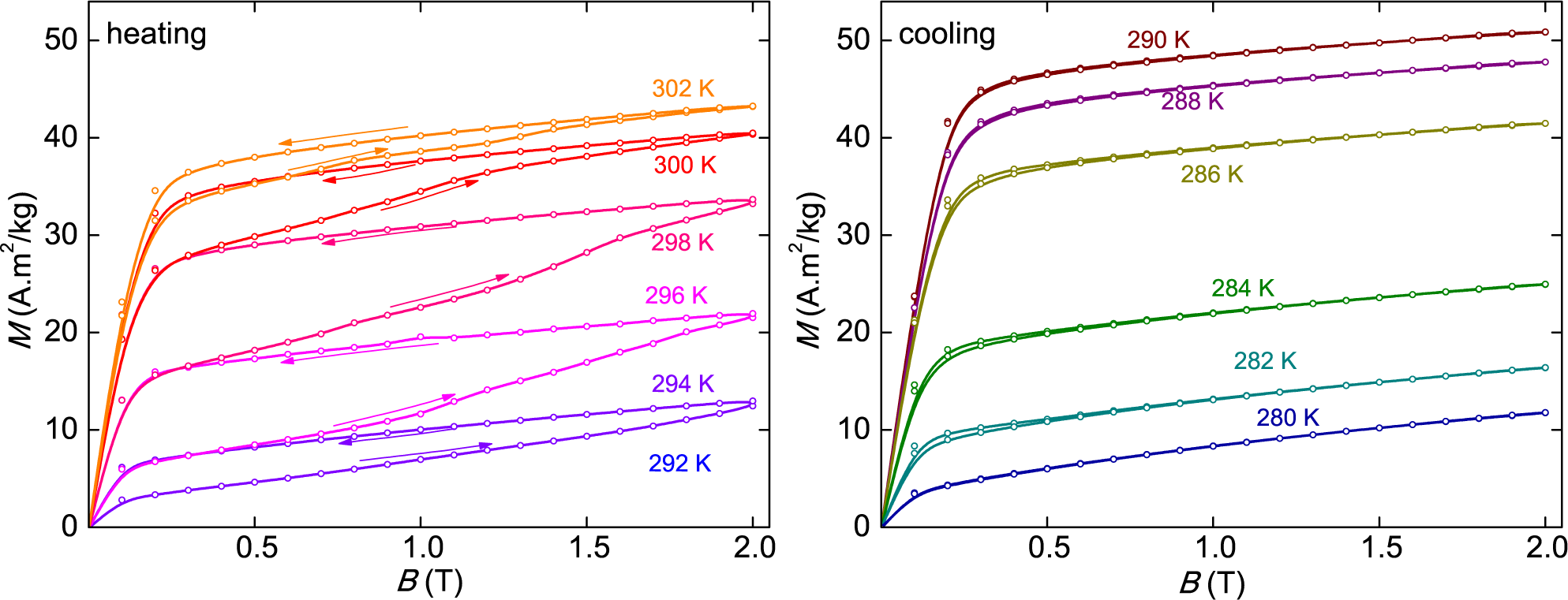For equal intervals, the field at which the phase conversion starts, B₂, is approximately the same for all isotherms, and B_m − B₂ is independent of B_m. This behavior of the present sample was clearly observed in our magnetic measurements, shown in Figure 3 (heating), and it is even more evident in the magnetization of the closely-related compound, Ni₅₀Mn_39.5In_10.5, taken at smaller temperature intervals, but reported without a correct explanation in Figure 3 of [18]. The measurements reported in that study indicate that the magnetization curve at each temperature, between 200 K and 210 K, overlaps the demagnetization curve of the previous temperature up to B₂ ≈ 9 kOeand then goes to higher values between B₂ and B_m. Considering that the sample, structurally being in the state of M, A or in a mixture of both states, has normal MCE and that only a small portion suffers phase conversion in each isotherm, the resulting ΔS_T can be negative or positive, depending on the temperature interval and the width of the transition band. In any case, ΔS_T is much lower than the total transition entropy jump for the sample determined from heat capacity or from the Clausius–Clapeyron equation.

Finally, the phase conversion ends when the state point exits the transition band, when crossing the A_f line at B₃. At the subsequent temperatures, the entropy variation corresponds to the normal MCE of the austenite.

It is worth remarking that, according to this analysis, in the similar protocol made on cooling, there should not be any phase conversion in the magnetization-demagnetization process. The transition takes place only on the cooling step at zero field, between the blue lines of Figure 2a. Our magnetization measurements shown in Figure 3 (cooling) give overlapping curves on the increasing and decreasing field, without any additional change in the fraction of M due to phase conversion, corroborating these arguments. This explains why in the direct measurement of ΔT_S, given in [14] and made always upon application of a field in a magnetization process, an IMCE is observed on heating, but a normal MCE is seen on cooling.

2.3. Protocol c: Heat Absorption on Isothermal Demagnetization

This is used for direct determinations of the absorbed heat on demagnetization, Q, to obtain the isothermal entropy change as −ΔS_T ≈ Q/T. This physical process is similar to protocol b, but the temperature increases are made at a constant field, B_m. Then, the field is decreased isothermally while measuring the heat absorbed to maintain T constant. The field is increased again up to B_m and the sample heated to a new temperature. Like in protocol b, there is no phase conversion from A to M on demagnetization for the field values used, but only from M to A on magnetization and on further heating to the next temperature, while the heat exchange is not recorded. As the measured quantity is the heat absorbed on demagnetization, it corresponds to the normal MCE of the mixture of the A and M phases existing at the initial point (T, B_m). Therefore, ΔS_T < 0, taken with the usual convention of ΔS_T = S(T, B_m) − S(T, 0).

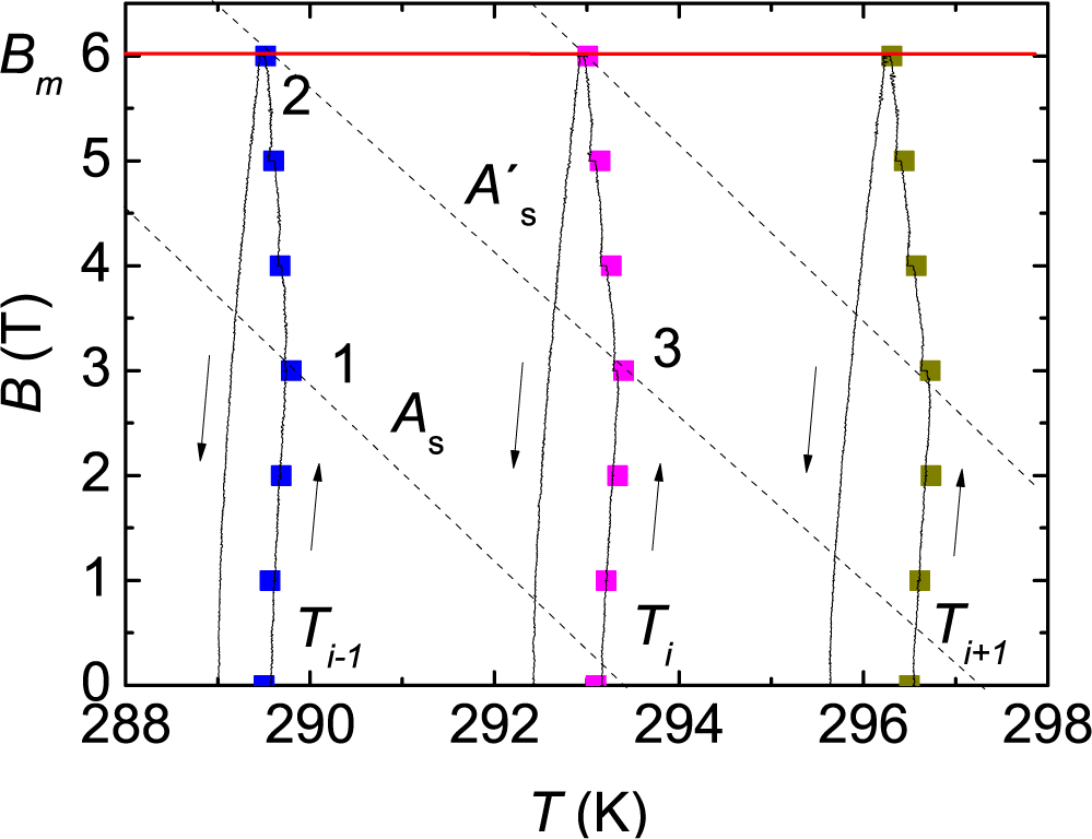
2.4. Protocol d: Adiabatic Magnetization Cycles

The field is increased and decreased adiabatically, and the temperature is recorded as a function of the field. Figure 4 shows the experimental data in some processes, starting at various consecutive temperatures. The continuous lines represent the experimental dynamic processes at field rates of 0.01 T/s and −0.01 T/s, and the symbols correspond to equilibrium points as described in [3]. In this case, when the field increases, the temperature initially increases due to the normal MCE of the pre-existent mixture of the M and A phases. Considering the adiabatic magnetization-demagnetization cycle starting at a temperature T_i, as shown in Figure 4, the trend changes when the phase conversion starts, which happens when the state point crosses the limiting transition line of the sample grains that did not transform in the previous magnetization runs and remained in the M state (Point 3 in Figure 4). This line is defined by the conversion line passing through the state point reached at the maximum field of the previous magnetization process (Point 2). After that, the temperature decreases until reaching the maximum field or until the M to A phase conversion is complete. On decreasing the field, there is no phase conversion, and the slope B − T is always positive. This general behavior was also observed in the field cycles around the reverse martensitic transition [19].

3. Heat Capacity and Direct Measurements of ΔS_T

3.1. Isothermal Entropy Change

The heat absorbed on demagnetization, Q, has been measured quasi-statically following protocol c. The details of the experimental device are described elsewhere [20]. The corresponding ΔS_T results are plotted in Figure 5. As explained when describing protocol c, there is no phase conversion on demagnetization due to the wide hysteresis. Consequently, ΔS_T corresponds to the normal MCE coming from the mixture of M and A phases, with a growing fraction of the A phase on increasing the temperature. The proportion of each phase in the sample changes along the transition band going from the pure M phase in the low temperature range to the pure A phase in the high temperature range of the measurements. In the mixed state, the value of ΔS_T can be estimated as ΔS_T,mix = (1 − x)ΔS_T (M) + xΔS_T (A). The normal MCE of the A phase, −ΔS_T (A), is expected to have a maximum near $T_C^A$, and similarly, −ΔS_T (M) is expected to have a maximum near $T_C^M$.

A rough estimation of these entropy contributions can be made by applying a sort of corresponding states law with a typical second-order transition compound, like Gd. The MCE of the pure austenite, for a field change of 3 T, has been estimated from the values obtained for Gd, multiplying the temperature by the scale factor $T_C^A/T_C$ (Gd) and the entropy change by another factor chosen to agree with the experimental ΔS_T at $T_C^A$. This gives the upper dashed line in Figure 5. Estimating in a similar way the normal ΔS_T of the martensite gives the lower dashed line in the same figure. The fraction x of the austenite can be taken to be proportional to the anomalous enthalpy of the M → A transition at each temperature and field, as deduced in Section 3.2. The curve ΔS_T,mix deduced in this way agrees remarkably well with the direct measurements of ΔS_T (3 T), as shown in Figure 5. This proves that this experiment allows one to determine the magnetic entropy increment of the mixed phase.

The direct measurements of the isothermal entropy change upon decreasing field, shown in Figure 5, have negative values, with a peak at 320 K that corresponds to the Curie temperature of the sample, being completely in the A phase at this temperature. Furthermore, the increase of −ΔS_T below 280 K agrees with the expected peak at $T_C^M$ in this region, when the sample is in the M phase.

3.2. Heat Capacity

The heat capacity, C_B, represented in Figure 6, was measured at constant fields in an adiabatic calorimeter following protocol a, using the conventional heat pulse method and also by continuous heating or cooling, as described in [21], using temperature rates around 2 mK/s. Table 1 contains the main relevant results of transition temperatures and anomalous entropies and enthalpies. Broad anomalies occur near the martensitic transition, indicating an inhomogeneous distribution of composition and microstructure in our rather large experimental sample (m = 1.56 g). These anomalies are much broader than the transitions found in the magnetic measurements done previously on a small piece of the same sample [14,16]. In addition, the Curie anomalies of the M and A phases are smeared out in the heat capacity results. This points to a distribution of T_C’s, which can be attributed to inhomogeneities in the composition. The transition temperatures have been assigned to the centroid of each broad anomaly, corresponding to 50% of M and A phases.

From the heat capacity, the entropy was determined as:

$$S(T,B)=S(T_0,B)+{\displaystyle {\int }_{T_0}^T\frac{C_B}{T}dT}$$

(4)

the integration constant S(T₀, B) has different values depending on B and has to be taken into account in computing the MCE from the C_B data. This constant was determined from the experimental entropy change, directly measured in the M phase, where the MCE is conventional and weak, $S(T_0,B)=\mathrm{\Delta }{S}_{T_0}(0\to B)+S_0(T_0,0)$. The values of $\mathrm{\Delta }{S}_{T_0}$ were obtained at T₀ = 273 K, and S₀(T₀, 0) is an absolute constant, irrelevant for the discussion here. The anomalous enthalpy, ΔH_an, and entropy, ΔS_an, at the martensitic transition were deduced from the area under C_an = C − C_b and C_an/T curves, where C_b is a common baseline that takes into account the smooth contributions to the heat capacity. The heat capacity data from the heat pulse method are systematically biased downwards near the first-order transition due to the long relaxation times in this region. Therefore, the ΔH_an and ΔS_an values deduced from the continuous measurements are more reliable for these transitions. Entropy curves for different fields were calculated from C_B(T) and are represented in Figure 7 for 0 and 6 T fields and heating measurements. One can see that the entropy at a high field is above the zero field entropy in the temperature range between 287 K and 305 K. The isothermal entropy increments were deduced from the relation ΔS_T = S(T, B) − S(T, 0) (Figure 8a). Similarly, the adiabatic temperature change was deduced from the inverted functions, T (S, B) as ΔT_S = T (S, B) − T (S, 0) (Figure 8b).

The state (T, B) in Figure 2a, reached through protocol a, is expected to be the same as if the process were made on heating at zero field up to (T, 0) and, then, increasing the field isothermally to (T, B). This follows from the assumption of reaching the same state at the point (T, B) when proceeding only in the same direction for the phase conversion, M to A in this case. In this field process, there is some phase conversion in the transition region. The entropy change is due to two competing effects, the normal and negative MCE of the mixture of M and A phases, and the positive entropy change of the transition that depends on the amount of sample converted. Therefore, the total −ΔS_T has a minimum and becomes even negative near T_MA, where the conversion is higher. Given the width of ≈ 30 K, shown by the C_B anomalies and the weak field dependence of the transition temperature of ≈ −1.1 K/T, it is clear that the complete transformation cannot occur at any temperature for a field change from 0 to 5 T. Moreover, the normal negative entropy change due to the magnetic contribution reduces the total entropy change. Therefore, ΔS_T will be much smaller than the transition entropy given in Table 1. The entropy change determined from the Clausius–Clapeyron equation has to agree with the data given in Table 1, except for a minor error due to the irreversibility. Actually, taking dB_t/dT_t = −0.93 T/K from the data given in Table 1 and ΔM = 35 A·m²/kg from [14], one obtains ΔS_an = 33 J/kg·K, in excellent agreement with the results from C_B. Of course, this agreement does not occur in the direct determination of ΔS_T following protocol c, in which there is no phase conversion and ΔS_T < 0 at every temperature.

We can make a more quantitative comparison considering the fraction of sample that transforms at each temperature under a field change. The initial fraction of the A phase, x₀, can be obtained from the anomalous enthalpy at zero field and corresponds to the point (T, 0) in Figure 2a indicated by the end of the lower arrow. Similarly, the final state corresponds to the point (T, B), indicated by the end of the upper arrow. The total conversion from phase M to phase A implies a latent heat, ΔH_an, so the converted fraction at a given temperature and field, x(T, B), can be taken as the anomalous enthalpy of this state normalized with the full transition enthalpy, $x(T,B)=(1/\mathrm{\Delta }{H}_{B,an}){\displaystyle {\int }_0^T{C}_{B,an}(T)dT}$ and $\mathrm{\Delta }{H}_{B,an}={\displaystyle {\int }_0^{\infty }{C}_{B,an}(T)dT}$. The maximum experimental difference, x(T, 5 T) − x(T, 0) = 0.20, was obtained at 296 K. Assuming the normal magnetic entropy change of the mixed phase as determined in the direct measurements on demagnetization at this temperature, ΔS_m(296 K) = −2.2 J/kg·K, and the anomalous entropy of the M to A transition, 30 J/kg·K, we can expect for the total entropy change with ΔB = 5 T, ΔS_T (296 K) = −2.2 + 0.20 × 30 = +3.8 J/kg·K, which agrees reasonably well with the value determined from the entropy curves, +2.7 J/kg·K.

4. Effect of the Distribution of Transition Temperatures

In the case of compounds with normal GMCE, the application of a magnetic field induces the paramagnetic to ferromagnetic phase change at temperatures above the spontaneous zero field transition temperature, T_C, and up to the transition temperature at the maximum applied field, $T_{C,B_m}$. Above $T_{C,B_m}$, the field is not strong enough to transform the sample to the ferromagnetic state. Considering that ΔS_T has a high value only when there is phase conversion, but is low in both the pure paramagnetic and the pure ferromagnetic phases, ΔS_T (T) would have a square shape for a sharp first-order transition, with a high plateau between T_C and $T_{C,B_m}$. The up and down jumps are more or less abrupt depending on the homogeneity of the sample. However, the top of the square is essentially independent of the homogeneity, provided that it corresponds to a complete phase transformation. Moreover, ΔS_T at the plateau must be equal on magnetization and on demagnetization, on heating and on cooling, because S is a state function, and its variation in a closed cycle is zero, since the sample returns to the same state. For inverse GMCE materials, there is a similar behavior, with the difference that the ferromagnetic state is the stable one at higher temperatures than the non-magnetic state.

For the present compound, there are significant differences. Considering the width of the transition, ≈ 30 K, and the field dependence of the transition temperature, ≈ −1 K/T, as seen in Figure 6 and Table 1, a field stronger than 30 T would be necessary to achieve the complete M to A phase conversion starting with the sample in the M state. For most practical accessible fields, the transition will always be partial on isothermal magnetization and similarly on demagnetization. The width of the transition band, given by the differences A_f −A_s and M_s−M_f, is affected by inhomogeneities in composition and temperature, internal stresses and atomic disorder. In our sample, DSC experiments on a finely powdered portion of the sample did not show any relevant change of the transition width, discarding any significant influence of the stress.

The width of the transition band explains many apparent inconsistencies in determinations of the MCE parameters, in particular ΔS_T. Looking at Figure 2b and considering the discussion of protocol b, it is evident that a determination of ΔS_T on an increasing field will depend on the temperature step between consecutive measurements and the width of the transition band. 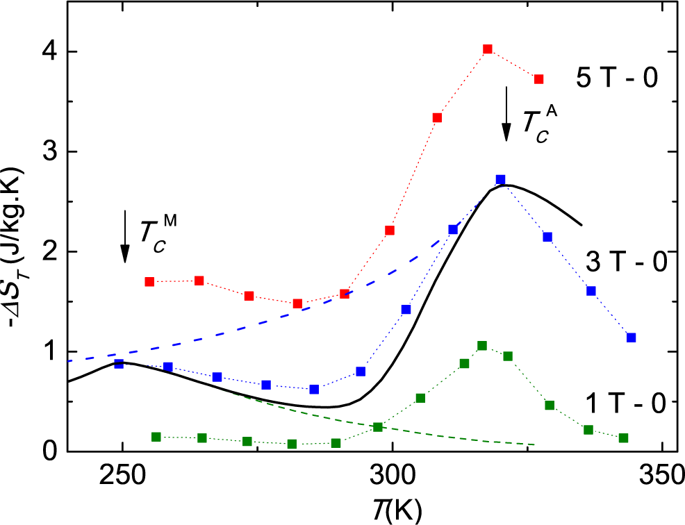The values obtained from isothermal magnetization measurements (protocol b), using the Maxwell relation, give a spurious contribution, as described in [22], but distributed along the whole transition band, where a partial phase conversion exists. On the other hand, the heat capacity data give precise values of the entropy change upon field changes, and the isofield magnetization measurements, on heating, give also correct results. Nevertheless, a comparison of the present heat capacity results (Figure 8) with previous deductions from isofield magnetization [14] differ by one order of magnitude. This difference can be explained quantitatively considering the actual width of the transition for each of the samples used in the experiments. The work in [14] reports a maximum ΔS_T (298K) = +10.4 J/kg·K for a field increment of 2 T, calculated from isofield magnetization on heating. From the magnetization curves reported in Figure 2 of this work, one can estimate a 40% conversion from M to A at 298 K for this field change. Considering this part of the total anomalous entropy for the M to A transition, given in Table 1, and the negative contribution of the normal magnetic entropy change, shown in Figure 5, one obtains ΔS_T (298K) ≈ −0.7+0.40×30 = 11.3 J/kg·K, in good agreement with the value deduced from the magnetization measurements [14]. The sample used in the present study is bigger and has a broader transition. Heat capacity determinations give only a maximum phase conversion of 20% for a field variation of 5 T, leading to much smaller entropy changes, as shown in Figure 8a. Therefore, the contradiction between the quite different ΔS_T values obtained for different samples is only apparent and can be quantitatively explained considering the different transition band widths of the samples.

5. Conclusions

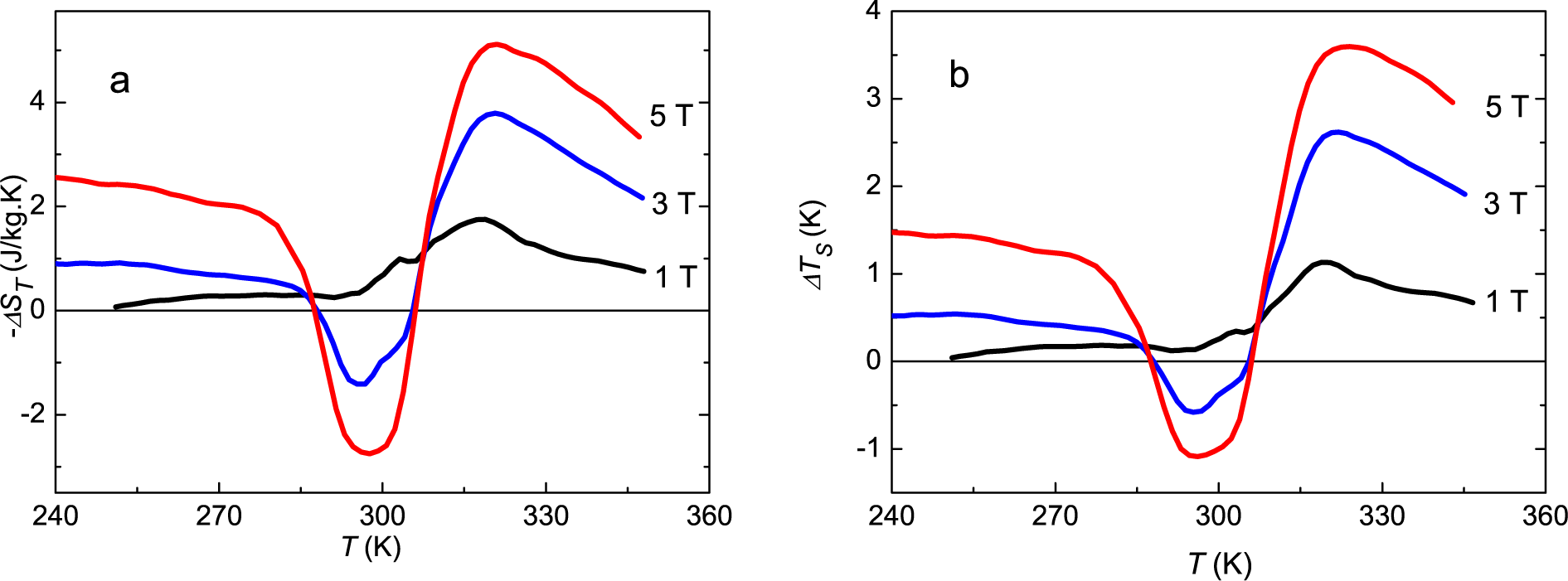
The apparently contradictory results for ΔS_T obtained from different techniques and samples have been explained when considering the path followed by the state point on the phase diagram, the measuring protocol, the hysteresis and the width of the transition for each sample.

Due to the large hysteresis, the direct determination of the isothermal entropy change on demagnetization gives the opportunity to determine independently the purely magnetic entropy increment of the mixture of martensite and austenite at each temperature. In our sample, these direct determinations gave positive values for −ΔS_T at every temperature, like in compounds with normal MCE.

The heat capacity at a constant field allows determining the entropy change at the transition involving magnetic, phonon and electronic contributions. Any other experimental data, like magnetization, needs an explanation of the protocol followed in the experiments to be able to obtain a reliable interpretation of the results. In any case, the isothermal or adiabatic magnetization and demagnetization in the transition region induce a partial phase conversion, and the thermal effect depends on the fraction converted. Depending on the state path followed in a direct measurement of ΔS_T, a different value can be obtained for ΔS_T (296K, ΔB = 5 T) between −2.2 J/kg·K and +3.8 J/kg·K, corresponding to the absence of any part of the sample changing phase and to the maximum phase conversion for this field, respectively. The experimental value depends on the temperature step used in the series of measurements. The data in Table 1 and in Figure 5, giving results for the martensitic transition and for the magnetic entropy changes, allow one to predict the results for any other protocols with a fair approximation.

Ni₅₀CoMn₃₆Sn₁₃ and some other related Heusler alloys offer the opportunity to have a large entropy change with low applied fields under appropriate conditions [23]. However, the actual compounds have serious drawbacks with regard to applications in magnetic refrigeration: (1) The sample conversion is never complete in moderate magnetic fields, due to the broad transition. Therefore, the entropy change is always lower, and, sometimes, even opposite in sign, than the expected change corresponding to the latent heat of the martensitic transition. (2) At temperatures at which the M to A transformation can be induced by a magnetic field, the large hysteresis prevents having the reverse transformation on demagnetization. Conversely, at temperatures at which the A to M transformation occurs on demagnetization, the applied field is not strong enough to achieve the M to A transformation. (3) Even if both previous difficulties were overcome with a very homogeneous sample having a sharp martensitic transition and a small hysteresis, the useful temperature span would be small. Due to the Clausius–Clapeyron equation and the relatively small magnetization change between the M to A phases compared to other GMCE materials, the transition line in a B − T diagram is very steep. Consequently, a given field increment produces a small shift of the martensitic transition temperature, allowing the occurrence of the transition and the GMCE only in a narrow temperature interval.