Hidden State Conditional Random Field for Abnormal Activity Recognition in Smart Homes

Abstract

As the number of elderly people has increased worldwide, there has been a surge of research into assistive technologies to provide them with better care by recognizing their normal and abnormal activities. However, existing abnormal activity recognition (AAR) algorithms rarely consider sub-activity relations when recognizing abnormal activities. This paper presents an application of the Hidden State Conditional Random Field (HCRF) method to detect and assess abnormal activities that often occur in elderly persons’ homes. Based on HCRF, this paper designs two AAR algorithms, and validates them by comparing them with a feature vector distance based algorithm in two experiments. The results demonstrate that the proposed algorithms favorably outperform the competitor, especially when abnormal activities have same sensor type and sensor number as normal activities.

1. Introduction

Smart homes are one realization of ambient intelligence (AmI) [1] which is emerging as an omnipresent computing technology that can anticipate people’s goals and intentions with contextual sensor data. As the number of elderly people in society increases, the need for assistive technologies in the home becomes more urgent [2]. As age-related changes in the brain cause a decline in short-term memory and slow learning ability, elderly people run into all sorts of barriers in performing their daily routine tasks [3]. Thus, to better care for elderly people, we not only need to know what they are doing, but also need to know if there are some abnormal activities [4]. Abnormal activity recognition (AAR) in smart home is an emerging technology that can help elderly residents live comfortably and safely by identifying unexpected and irregular events [5], e.g., falls or taking medicine many times in a short time.

Over the last decade, there has been a considerable research on AAR in smart homes. However, most of it is based on cameras [6,7], wearable sensors [8,9] and RFID sensors[10,11], and studies on AAR in AmI environments using non-obtrusive and pervasive sensors are rare. In 2007 and 2008, Jakkula et al. [12,13] proposed recognizing abnormal activities using non-obtrusive sensors. In their research, they used temporal logic (before, after, meets, overlaps, starts …) to identify temporal relationships between events and detected anomalies by calculating the probability of a given event occurring or not occurring. However, this method needs a long time to learn all the temporal relations and events grouped together are only from the same device. In 2011, Jakkula et al. [14] also proposed recognizing abnormal activities based on a One-class Support Vector Machine (One-class SVM), and later Lotfi et al. [15] proposed recognizing abnormal activities in smart homes based on a clustering and neural networks method, but neither both of them can model the temporal relationships between activities. In 2014, Wang et al. [16] defined abnormal activity as an activity which deviates greatly enough from those normal activities, and recognized abnormal activities using a distributed abnormal activity detection approach which employs the computing and storage resources of simple and ubiquitous sensor nodes, but they cannot deal with abnormal activities which deviate only a little from those normal activities. In the same year, Zhao et al. [5] proposed a Markov Chains Model-based method to classify abnormal sequences by analyzing the probability distribution of the spatiotemporal activity data, but the sensors used were only infrared sensing tubes. Mahmoud et al. [17] proposed a hybrid technique for user activity outlier detection which consists of a two-stage integration of principal component analysis and fuzzy rule-based systems.

Nowadays, there are still some difficulties to recognize abnormal activities in smart homes. First of all, since abnormal activities are often unknown in advance and many types of abnormal activities occur very infrequently, it is often hard to obtain samples to train the abnormal activity recognition model. Furthermore, even if there are some examples known as anomalous, they may not represent the underlying distribution of that class accurately, making them unsuitable as training data. Secondly, it is hard to recognize sequential abnormal activities. Some abnormal activities are sequentially anomalous, in particular, an anomalous pattern is often defined as a series of events that are normal individually but abnormal only collectively. For example, toileting is a common and expected activity, but a frequent repetition in a short time may indicate something anomalous. It is well known that activities and abnormal activities are often composed by several sub-activities, especially complex activities, e.g., washing the hands implies the following sub-steps: move to the kitchen (or bathroom), turn on water, use hand soap, wash hands, dry hands. Also, individuals may complete one activity in different ways, e.g., making a phone implies the following variants: sits down during conversation, stands in one place during conversation, or walks around during the phone call. These actions and different ways are the intrinsic sub-structures of the whole activity.

A number of algorithms have been proposed to recognize sequential activities based on Conditional Random Field (CRF) [18–20] and to recognize objects and gestures based on Hidden Conditional Random Field (HCRF) [21,22]. However, abnormal activities are not predictable and annotating them all in advance is infeasible, which thus suggests the need for a recognition algorithm for sequential AAR. Considering the activity characteristic, this paper proposes using HCRF to improve the AAR accuracy by modeling relations between sub-activities.

HCRF expands CRF by incorporating hidden state variables which can model the sub-structures of a sequence. CRF is a sequence probabilistic graphical model and can be used for sequence labeling [23]. CRF can be understood as a sequential extension to the Maximum Entropy Model (MEM) [24] and its main idea is the MEM [25], which models all that is known and assumes nothing about what is unknown. HCRF is a sequence probabilistic graphical model which introduces probability calculus and statistical inference, and takes root in MEM. It can capture internal substructures and model context relations of sub-activities by detecting causal dependencies from data.

The remainder of this paper is organized as follows: firstly, HCRF that is used for AAR will be presented. Then, two AAR algorithms based on HCRF will be described. After recognizing normal activities using HCRF, we validate our algorithms and discuss the results. Finally, we conclude by summing up our findings.

2. Hidden Conditional Random Field

HCRF takes root in CRF [26], which has been proved equivalent to the MEM [25]. Both CRF and HCRF can be used for sequence labeling. For every time step t=1, 2, ···, T, CRF consists of sequential variable pairs of state variables y_t and observable variables x_t, and can capture extrinsic dynamics between activity labels. HCRF is an undirected graph model and it can be used for labeling segmented sub-sequence. For each local observation vector x={x₁, x₂,···, x_T}, HCRF assumes that there are one state label y ∈ Y, Y={1,2,···,K}and a vector h={h₁, h₂,···, h_T}, where _ht ∈ _H, _t=1,2,···,T and H is a finite set of possible hidden labels in the model. The Graphical structure of CRF and HCRF are shown in Figure 1(a) and Figure 1(b).

We can only observe vector x={x₁, x₂,···, x_T} and state label y in the training dataset. Since the variables h₁, h₂,···, h_T are not observed, they are called hidden state variables in the model. The number of hidden states (NH) in H is decided at the training stage by minimizing the error of the training data [27]. HCRF is discriminative model and it models conditional probability using feature functions like MEM. Given an observation vector x, it defines a conditional probabilistic model as:

$$P\left(y,\mathit{h}|\mathit{x},\mathit{\theta }\right)=\frac{e^{\mathrm{\Psi }(y,\mathit{h},\mathit{x};\mathit{\theta })}}{{\displaystyle {\sum }_{y^{\prime },\mathit{h}}{e}^{\mathrm{\Psi }(y^{\prime },\mathit{h},\mathit{x};\mathit{\theta })}}}$$

(1)

where θ is the parameters of the model, $\mathrm{\Psi }(y,\mathit{h},\mathit{x};\mathit{\theta })\in R$ is potential function defined in Maximum Entropy Model and parameterized by θ.

Given an observation vector x and all possible hidden state variables h, it follows that:

$$P\left(y|\mathit{x},\mathit{\theta }\right)={\displaystyle \sum _{\mathit{h}}P\left(y,\mathit{h}|\mathit{x},\mathit{\theta }\right)}=\frac{{\displaystyle {\sum }_{\mathit{h}}{e}^{\mathrm{\Psi }(y,\mathit{h},\mathit{x};\mathit{\theta })}}}{{\displaystyle {\sum }_{y^{\prime },\mathit{h}}{e}^{\mathrm{\Psi }(y^{\prime },\mathit{h},\mathit{x};\mathit{\theta })}}}$$

(2)

We now turn to the definition of the potential function $\mathrm{\Psi }(y,\mathit{h},\mathit{x};\mathit{\theta })$ which is very important for HCRF. We assume an undirected graph structure, with the hidden variables h={h₁, h₂,···, h_T} and corresponding to vertices in the graph. We use E to denote the set of edges in the graph, and (j,k)∊ E to signify that there is an edge in the graph between variables h_j and h_k. With this definition, the potential function takes the following form [21]:

$$\mathrm{\Psi }(y,\mathit{h},\mathit{x};\mathit{\theta })={\displaystyle \sum _{j=1}^T{\displaystyle \sum _l{f}_l^1(j,y,h_j,\mathit{x}){\theta }_l^1}+{\displaystyle \sum _{(j,k)\in E}{f}_l^2(j,k,y,h_j,h_k,\mathit{x}){\theta }_l^2}}$$

(3)

where $f_l^1,f_l^2$ are functions defining the features in the model, and ${\theta }_l^1,{\theta }_l^2$ are the components of $\mathit{\theta }$.

In the model, feature $f_l^1$ depends on single hidden variable values and models the relation between observation and hidden variable, while feature $f_l^2$ depends on pairs of values and models the relation between two hidden variables.

Given a new test x, HCRF infers label y by $\arg {\max }_{y\in Y}P(y|\mathit{x},{\mathit{\theta }}^{*})$, where θ^* is parameters of the model that estimated trained using training dataset.

2.1. Parameter Estimation

Following CRF [23], we use the following objective function in training the parameters:

$$L(\mathit{\theta })={\displaystyle \sum _i\log P\left(y_i|{\mathit{x}}_i,\mathit{\theta }\right)}-\frac{1}{2{\sigma }^2}{\Vert \mathit{\theta }\Vert }^2$$

(4)

where the first term of Equation (4) is the log-likelihood of the data, and the second term is the log of a Gaussian prior with variance σ², i.e., $P(\mathit{\theta })\sim \frac{1}{2{\sigma }^2}{\Vert \mathit{\theta }\Vert }^2$.

This work lets ${\mathit{\theta }}^{*}=\arg {\max }_{\mathit{\theta }}L(\mathit{\theta })$ and uses a gradient ascent to search for the optimal parameter values. In this section we describe how the gradient of L(θ) can be calculated efficiently. Consider the likelihood term that is contributed by the i-th training example, defined as:

$$L_i(\mathit{\theta })=\log P\left(y_i|{\mathit{x}}_i,\mathit{\theta }\right)=\log \left(\frac{{\displaystyle {\sum }_{\mathit{h}}{e}^{\mathrm{\Psi }(y_i,\mathit{h},{\mathit{x}}_i;\mathit{\theta })}}}{{\displaystyle {\sum }_{y^{\prime },\mathit{h}}{e}^{\mathrm{\Psi }(y^{\prime },\mathit{h},{\mathit{x}}_i;\mathit{\theta })}}}\right)$$

(5)

We first consider derivatives with respect to the parameters ${\theta }_l^1$ corresponding to features $f_l^1$ that depend on single hidden variables. Taking derivatives gives:

$$\begin{array}{l}\frac{\partial L_i(\mathit{\theta })}{\partial {\theta }_l^1}={\displaystyle \sum _{\mathit{h}}P(\mathit{h}|y_i,{\mathit{x}}_i,\mathit{\theta })}\frac{\partial \mathrm{\Psi }(y_i,\mathit{h},{\mathit{x}}_i;\mathit{\theta })}{\partial {\theta }_l^1}-{\displaystyle \sum _{y^{\prime },\mathit{h}}P(y^{\prime },\mathit{h}|{\mathit{x}}_i,\mathit{\theta })\frac{\partial \mathrm{\Psi }(y^{\prime },\mathit{h},{\mathit{x}}_i;\mathit{\theta })}{\partial {\theta }_l^1}}\\ ={\displaystyle \sum _{\mathit{h}}P(\mathit{h}|y_i,{\mathit{x}}_i,\mathit{\theta })}{\displaystyle \sum _{j=1}^T{f}_l^1(j,y_i,h_j,{\mathit{x}}_i)}-{\displaystyle \sum _{y^{\prime },\mathit{h}}P(y^{\prime },\mathit{h}|{\mathit{x}}_i,\mathit{\theta }){\displaystyle \sum _{j=1}^T{f}_l^1(j,y^{\prime },h_j,{\mathit{x}}_i)}}\\ ={\displaystyle \sum _{j,a}P(h_j=a|y_i,{\mathit{x}}_i,\mathit{\theta })}{f}_l^1(j,y_i,a,{\mathit{x}}_i)-{\displaystyle \sum _{y^{\prime },j,a}P(y^{\prime },h_j=a|{\mathit{x}}_i,\mathit{\theta })f_l^1(j,y^{\prime },a,{\mathit{x}}_i)}\end{array}$$

(6)

Equation (6) can be expressed in terms of components $P(h_j=a|{\mathit{x}}_i,\mathit{\theta })$ and $P(y|{\mathit{x}}_i,\mathit{\theta })$ which can be calculated using belief propagation [28]. A similar calculation gives:

$$\begin{array}{l}\frac{\partial L_i(\mathit{\theta })}{\partial {\theta }_l^2}={\displaystyle \sum _{(j,k)\in E,a,b}P(h_j=a,h_k=b|y_i,{\mathit{x}}_i,\mathit{\theta })f_l^2(j,k,y_i,a,b,{\mathit{x}}_i)}\\ -{\displaystyle \sum _{y^{\prime },(j,k)\in E,a,b}P(h_j=a,h_k=b,y^{\prime }|{\mathit{x}}_i,\mathit{\theta })f_l^2(j,k,y^{\prime },a,b,{\mathit{x}}_i)}\end{array}$$

(7)

where $P(h_j=a,h_k=b|y,\mathit{x},\mathit{\theta })$ can also be computed efficiently using belief propagation. For $\forall y\in Y,j\in 1,2,\cdots ,T,$$(j,k)\in E$, $a,b\in H$, belief propagation can be used to calculate the following quantities in $O(\left|E\right|\left|Y\right|)$ time:

$$Z(y|\mathit{x},\mathit{\theta })={\displaystyle \sum _{\mathit{h}}\exp \{\mathrm{\Psi }(y,\mathit{h},\mathit{x};\mathit{\theta })\}},\forall y\in Y$$

(8)

$$P\left(h_j=a|y,\mathit{x},\mathit{\theta }\right)={\displaystyle \sum _{\mathit{h}:h_j=a}P(\mathit{h}|y,\mathit{x},\mathit{\theta })}$$

(9)

$$P\left(h_j=a,h_k=b|y,\mathit{x},\mathit{\theta }\right)={\displaystyle \sum _{\mathit{h}:h_j=a,h_k=b}P(\mathit{h}|y,\mathit{x},\mathit{\theta })}$$

(10)

Z(y|x,θ) in Equation (8) is a partition function defined by a summation over the h variables and it can be used to calculate $P(y|\mathit{x},\mathit{\theta })=Z(y|\mathit{x},\mathit{\theta })/{\displaystyle {\sum }_{y^{\prime }}Z(y^{\prime }|\mathit{x},\mathit{\theta })}$. Equations (9) and (10) are marginal distributions over individual variables hj or pairs of variables h_j, h_k. Thus the gradient of L_i(θ) can be defined in terms of these marginal, and hence can be calculated efficiently. In our experiments, we performed gradient ascent with the BFGS optimization technique [29].

2.2. Inference

After the parameters θ^* are trained, the aim of HCRF is to infer the label y of a new test x by $\arg {\max }_{y\in \mathrm{Y}}P\left(y|\mathit{x},{\mathit{\theta }}^{\ast }\right)$. For K possible states of label y, it first calculates P(y = i|x,θ*) to get a K likelihood value l_i, i =1,2,…,K. After that, we make up this K likelihood value as one likelihood vector L ={l₁,l₂,⋯,l_K}, and denote index of the likelihood value in L as the likelihood value index. Then, we find the maximum likelihood value (MLV) of L and denote the index of the MLV in L as the MLV index. By finding the MLV index in L, we can find the optimal label. For example, the MLV of likelihood vector (1.5, 3.1, 2.5) is 3.1. Since the index of the MLV 3.1 in (1.5, 3.1, 2.5) is 2, the corresponding optimal label is 2.

3. Abnormal Activity Recognition Algorithm Based on HCRF

There are many kinds of abnormal activities in a smart home and there can be abnormality in time, places, frequency and duration. For example, sleeping on the floor and sleeping at eating time are abnormal activities with wrong place and wrong time. Toileting frequently and showering too long are abnormal activities with wrong frequency and duration. Also, there are abnormal activities that occur often and can be expected in advance and there are abnormal activities that occur rarely and are not expected in advance. “Resident does not get up on time” is an expected abnormal activity if a resident has not got up on time before, and “Falling” is an unexpected abnormal activity if a resident has not fallen before. This section focuses on “forgetting” and “new activity” abnormal activities that often occur in elderly homes.

To assess a new activity, we often compare it with normal activities [16,30]. Thus, a model that can compare normal activity and new activity is important for abnormal activity recognition. Considering HCRF one can model the similarity between a testing sample and training labels, so we proposed to recognize abnormal activities based on HCRF, and use a likelihood vector to represent the similarity between the testing activity and every type of training activity, using the MLV index to represent the most similar training activity, and using MLV to represent the similar value between a testing activity and the most similar training activity.

In our AAR algorithm, the purpose of HCRF is not to find activity labels, but to compute activity consistents and find abnormalities. Figure 2 gives the framework of AAR based on HCRF.

As Figure 2 shows, there are two stages in our AAR algorithm, the model building stage and the abnormal activity recognition stage. In the model building stage, we first build and train HCRF using all kinds of normal activities. Then, we infer the likelihood vector of all kinds of normal activities using the trained HCRF model and put the MLV of each type of normal activity in sets S_k, k =1,2, ⋯,K. Finally, we save the trained HCRF model and the MLV sets of each type of normal activity. In the abnormal activity recognition stage, we first infer the likelihood vector of the testing activity based on the trained HCRF and the testing activity observation sequence. Then, we find out the MLV V and MLV index i of the testing activity. Finally, we find any abnormality by comparing MLV V of the testing activity and MLV of the training activity that correspond to the MLV index i.

Given MLV V_t of a testing activity observation sequence t and MLV V_Ni of the most similar normal activity i, we assess testing activity by:

$$F_{normal}(t)=\left(1-\frac{\left|V_t-V_{Ni}\right|}{V_{Ni}}\right)\times 100$$

(11)

Obviously, for any testing activity, there is F_normal ∈ [0,100], and the larger the F_normal value is, the more similar it is to a normal activity i. To decide if the testing activity is an abnormal activity, we set a threshold γ. The value of γ is decided by the degree of abnormal activities we want to recognize. If F_normal > γ, the testing activity observation sequence is deemed as a normal activity and consistent with the most similar normal activity i, otherwise, the testing activity observation sequence t is deemed as an abnormal activity.

Next, we will give two types of abnormal activity recognition algorithms based on HCRF. To find abnormal activities with small differences with normal activities, we set γ = 98. The first type of abnormal activity we focused on is “forgetting” activities. Since this type of abnormal activity is often abnormal in sequence, we call them sequence abnormal activities. Algorithm 1 gives the procedure of sequence AAR based on HCRF.

Algorithm 1. The procedure of sequence AAR based on HCRF.00

Input: (1) Normal activity observation vectors and corresponding activity labels: (xn,yn), n =1,2,⋯,N0;  (2) Abnormal activity that corresponding to every kind normal activity;  (3) Observation vector of new activity.

Output: Normal or abnormal type.

1. Train HCRF using (xn,yn), $({\mathit{x}}^n,y^n)$, n =1,2,⋯,N0;

2. Compute the likelihood vectors of all normal activities based on trained HCRF, find out all the MLVs of the k-th normal activity, and puts the MLVs in to the normal MLV sets Sk,k= 1,2,⋯,K;

3. For observation vector of new activity, compute the likelihood vector based on trained HCRF, and find out MLV V and MLV index i;

4. Compute Fnormal. using Equation (11) based on Si. If Fnormal > 98, the activity is normal, turn step 6; otherwise, the activity is abnormal and turn step 5;

5. Check the abnormal type by comparing with the i-th type normal activity;

6. Output

Algorithm 1. The procedure of sequence AAR based on HCRF.00

Input: (1) Normal activity observation vectors and corresponding activity labels: (xn,yn), n =1,2,⋯,N0;  (2) Abnormal activity that corresponding to every kind normal activity;  (3) Observation vector of new activity.

Output: Normal or abnormal type.

1. Train HCRF using (xn,yn), $({\mathit{x}}^n,y^n)$, n =1,2,⋯,N0;

2. Compute the likelihood vectors of all normal activities based on trained HCRF, find out all the MLVs of the k-th normal activity, and puts the MLVs in to the normal MLV sets Sk,k= 1,2,⋯,K;

3. For observation vector of new activity, compute the likelihood vector based on trained HCRF, and find out MLV V and MLV index i;

4. Compute Fnormal. using Equation (11) based on Si. If Fnormal > 98, the activity is normal, turn step 6; otherwise, the activity is abnormal and turn step 5;

5. Check the abnormal type by comparing with the i-th type normal activity;

6. Output

The second type of abnormal activity we focused on is “new” activities. Since these are activities that have not happened before, we call this kind abnormal activity a rare abnormal activity. Algorithm 2 gives the procedure for rare AAR based on HCRF.

Algorithm 2. The procedure of rare AAR based on HCRF

Input: (1) Normal activity observation vectors and corresponding activity labels: (xn,yn), n =1,2,⋯,N0;  (2) Observation vector of new activity.

Output: Normal or abnormal.

1. Train HCRF using (xn,yn), n =1,2,⋯,N0;

2. Compute the likelihood vectors of all normal activities based on trained HCRF, find out all the MLVs of the k-th normal activity, and puts the MLVs in to the normal MLV sets Sk,k= 1,2,⋯,K;

3. For observation vector of new activity, compute the likelihood vector based on trained HCRF, and find out MLV V and MLV index i;

4. Compute Fnormal using Equation (11) based on Si. If Fnormal >98, the new activity is deemed as normal activity, otherwise, it is deemed as abnormal activity.

5. Output

Algorithm 2. The procedure of rare AAR based on HCRF

Input: (1) Normal activity observation vectors and corresponding activity labels: (xn,yn), n =1,2,⋯,N0;  (2) Observation vector of new activity.

Output: Normal or abnormal.

1. Train HCRF using (xn,yn), n =1,2,⋯,N0;

2. Compute the likelihood vectors of all normal activities based on trained HCRF, find out all the MLVs of the k-th normal activity, and puts the MLVs in to the normal MLV sets Sk,k= 1,2,⋯,K;

3. For observation vector of new activity, compute the likelihood vector based on trained HCRF, and find out MLV V and MLV index i;

4. Compute Fnormal using Equation (11) based on Si. If Fnormal >98, the new activity is deemed as normal activity, otherwise, it is deemed as abnormal activity.

5. Output

The two algorithms both train HCRF using all kind of normal activities. Then, based on trained HCRF, they compute the likelihood vectors of all kinds of normal activities and put the MLV into the normal MLV sets S_k,k= 1,2,⋯,K. For a new activity, they first compute the likelihood vector based on trained HCRF, and find out the MLV V and MLV index i. Then, they compute $F_{normal}$ using Equation (11) based on S_i. If F_normal >98, the activity is deemed a normal activity, otherwise, the activity is deemed an abnormal activity. The difference between them is that Algorithm 1 still needs to check the abnormal type by comparing with the i-th type normal activity. For many training normal activities, there will be many MLV for each S_k. For this case, we compute the consistent of V and S_i using Least-squares Approach [31] or One-class SVM [14].

4. Experiments

This section will describe three experiments. Firstly, we will validate HCRF in recognizing normal activities using a benchmark normal dataset “WSU Apartment Test bed, ADL adlnormal” which is collected in a smart apartment testbed located on the WSU campus [32]. Then, since there is no open source database about abnormal activities using non-obtrusive sensors, we do experiments with abnormal activities that were generated based on the above normal dataset in the next two AAR experiments.

The “WSU Apartment Test bed, ADL adlnormal” dataset was gathered by Diane Cook to recognize and assess the consistency of Activities of Daily Living that individuals perform in their own homes. There are 24 residents who performed five activities in a smart apartment testbed located on the WSU campus. Sensors in the apartment include monitor motion sensors (M), temperature sensors (T), water sensors (W), burner sensors (B), phone sensors (P), and item sensors (I). The motion sensors are located on the ceiling approximately 1 meter apart to locate the resident, the Voice over IP (VOIP) technology captures phone usage and switch sensors to monitor usage of the phone book, a cooking pot, and the medicine container. The five activities include both basic and more complex ADLs that are found in clinical questionnaires and are listed as follows:

• Telephone Use: Look up a specified number in a phone book, call the number, and write down the cooking directions given on the recorded message.
• Hand Washing: Wash hands in the kitchen sink.
• Meal Preparation: Cook oatmeal on the stove according to the recorded directions, adding brown sugar and raisins (from the kitchen cabinet) once done.
• Eating and Medication Use: Eat the oatmeal together with a glass of water and medicine.
• Cleaning: Clean and put away the dishes and ingredients.

Figure 3 is the performing routes of the five normal activities, where Ai presents the i-th activity. From the figure we can see that the activities 2–5 are very similar, while the activity 1 “Make a phone call” is very different from them.

4.1. Experiment 1

This experiment is designed to validate the HCRF model in recognizing normal activities. The adlnormal dataset includes sensor event data for 24 individuals who were asked to perform the five ADL activities, yielding a total of 120 activity traces containing 6425 sensor events (time slices). We train the HCRF model using the previous 5000 time slices and the trained HCRF model is applied on the next 1425 time-slices using a sliding window of fixed size. The class label with the highest likelihood is assigned to the frame at the center of the sliding window. The number of hidden states (NHS) and the length of the sliding window size (LW) are decided at the training stage. We assess the HCRF activity recognition results with a multi-class classification measure [33] which included average accuracy, error rate, precision, recall, f-score. Also, Support Vector Machine (SVM) [34,35] is supplemented for comparison purposes in the experiment.

Table 1. The result for Support Vector Machine (SVM) and Hidden Conditional Random Field (HCRF) models with the measures for multi-label classification.

	SVM	HCRF(NHS= 5, NW= 40)
Average Accuracy	0.8712	0.9258
Error Rate	0.1288	0.0742
Precision	0.7076	0.7710
Recall	0.5535	0.7987
F-score	0.3106	0.3923

is the result for the SVM and HCRF models with the measures for multi-label classification, where NHS is the number of hidden states and LW is the length of the sliding window size. From the table we can see that HCRF achieves a higher average accuracy, precision, recall, f-score and lower error rate than SVM, thus HCRF can better recognize normal activities. This is because HCRF can capture the intrinsic sub-structures of activity sequence and can encode the dynamics of the actions, while SVM only can model the activity feature in the same time slice and cannot encode the dynamics of actions. Also, Figure 4 compares the recognition accuracy for the SVM and HCRF models in the five activities from which we can see the recognition accuracies of HCRF get better results than SVM in four out of five activities. For the activity “Wash-hands”, SVM performs better than HCRF, this is because the activity involves little sensor activity and its sub-structure is minimal, thus modeling the sub-structure of this activity cannot help the activity recognition.

4.2. Experiment 2

In next two experiments, a feature vector distance based algorithm is used for AAR for comparing with the results of the HCRF-based the algorithms. The algorithm is essentially a simple clustering based abnormal activity recognition method [10,11] and they both find abnormalities by comparing the testing activity with the normal activity. The feature vector distance-based algorithm uses the activity feature vector distance to measure the activity similarity. The activity feature vector is expressed by the change sensors and is a vector with dimensions equal to the sensor number. When one activity is carrying out, if the i-th sensor state is changed, the i-th value of the activity feature vector is denoted as 1, otherwise, the i-th value of the activity feature vector is denoted as 0. For two activity feature vectors $A_i=(a_i^1,a_i^2,\cdots ,a_i^N)$ and $A_j=(a_j^1,a_j^2,\cdots ,a_j^N)$, the distance between them is computed using the corresponding Euclidean distance:

$$d(A_i,A_j)=\sqrt{\left({\displaystyle \sum _{n=1}^N{(a_i^n-a_j^n)}^2}\right)}$$

(12)

where N is the sensor number.

We use a method similar to the HCRF-based AAR algorithm to decide if the testing activity is abnormal. Given an activity feature vector A_t of testing activity observation sequence t and activity feature vector A_Ni of the most similar normal activity i, we assess testing activity by:

$$F_{normal}(t)=\left(1-\frac{d(A_t,A_{Ni})}{\Vert A_{Ni}\Vert }\right)\times 100$$

(13)

Also, there is F_normal ∈[0,100] for any testing activity. This experiment focuses on the recognition of “forgetting” abnormal activities and

Table 2. Seven abnormal activities.

Abnormal activity	Appearance	Sensor appearance
1. Make a phone call	Look in phone book twice	I08 give two ABSENT and PRESENT states
2. Wash hands	Forget to turn off the tap	AD1-B senses water flow when M18 gives state OFF
3. Cook1	Forget to replace spices	I01, I02, I03, I05 do not give state PRESENT
4. Eat1	Forget to take medicine	There are no states change for I06
5. Clean	Forget to clean dishes	AD1-B does not sense water flow
6. Cook2	Forget to turn off the microwave	AD1-A senses water flow when M14 give state ON and M17 give state OFF
7. Eat2	Take the medicine twice	I06 give two ABSENT and PRESENT states

lists seven abnormal activities generated based on the five normal activities, where the first abnormal activity is generated by the first normal activity, the second abnormal activity is generated by the second normal activity, the third and the six abnormal activities are generated by the third normal activity, the four and the seven abnormal activities are generated by the fourth normal activity, the fifth abnormal activity is generated by the fifth normal activity. To validate Algorithm 1, we recognize abnormal activities based on Algorithm 1 and the feature vector distance, respectively.

According to Algorithm 1, we first train HCRF using normal activities 1–5 and then compute their likelihood vectors based on the trained HCRF. The MLV and MLV index of normal activities 1–5 are (1, 326), (2, 100), (3, 573), (4, 195) and (5, 364), where the first value in brackets are the MLV indexes, and the second value in brackets are the MLVs.

For each testing activity, we compute the likelihood vector of the observation sequence based on the trained HCRF, and find out the MLV and MLV index. The likelihood vectors of testing activities 1–7 are shown in

Table 3. Likelihood vectors of seven sequences with HCRF.

Testing activities	Likelihood vectors (HCRF, NHS=6)
1	(438.6745, 409.2975, 398.6318, 32.4444,370.9995)
2	(183.4544, 194.3961,191.3976, 188.1670, 91.9349)
3	(790.0633, 839.4842, 842.2406, 28.0053,841.0192)
4	(148.7053, 143.4191, 134.0438, 150.5547,131.7339)
5	(347.8836, 375.7072, 372.7866, 370.8800,377.1156)
6	(888.2495, 943.2903, 948.6662, 929.4592, 3.2157)
7	(366.4750, 372.8574, 363.0768, 378.3354, 3.6117)

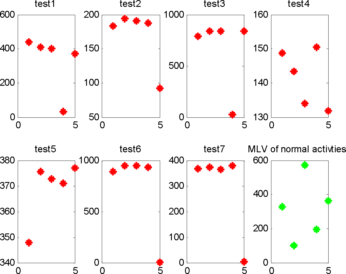
, where the first column represents the testing activities, and the second column represents the likelihood vectors. The likelihood vectors in this table represent the similarity between testing activities 1–7 and normal activities 1–5. Figure 5 is the visualization of the likelihood vectors of seven testing sequences and the MLV of five normal activities from which we can find out the MLV index of testing activities. Then, we determine whether the testing activity is abnormal using Equation (11). For instance, since the MLV index of testing activity 1 is 1, we consider testing activity 1 is most similar with normal activity 1. Computing F_normal using the MLV 438.6745 of testing activity 1 and the MLV 326 of the saved normal activity 1, we get F_normal = 65.43 < 98. Thus, we judge the testing activity 1 is an abnormal activity generated by the activity “Make a phone call”.

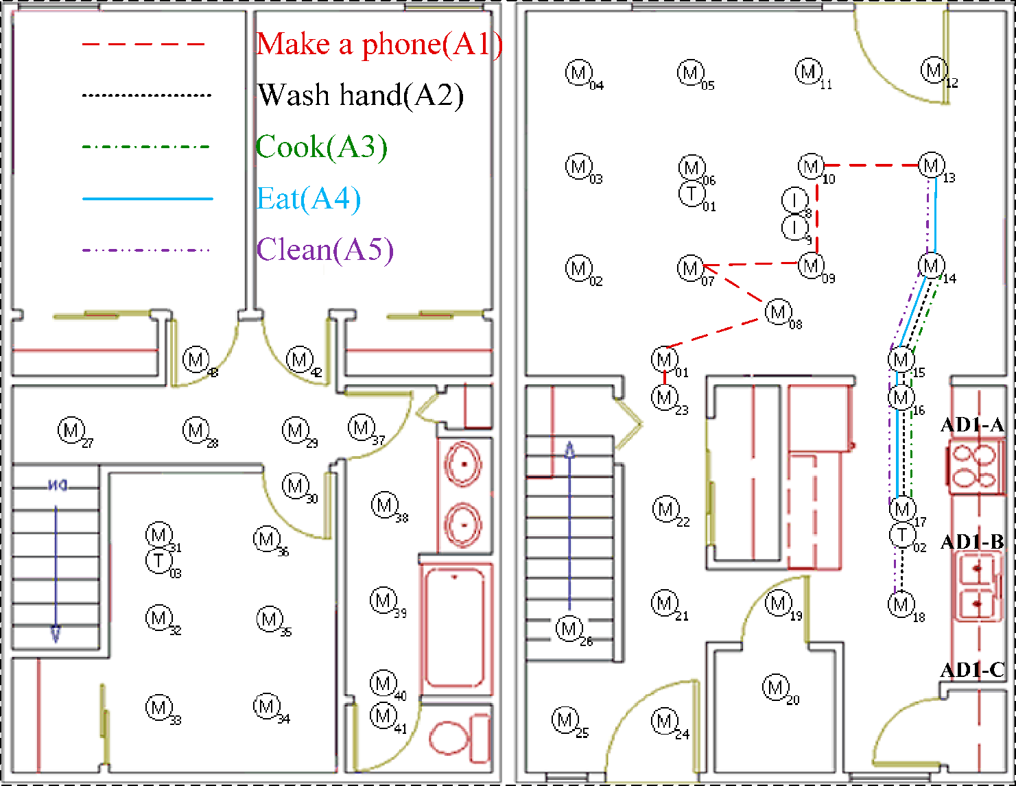
Finally, we find out the abnormal type by analyzing the observation sequence of testing activity. For instance, since the MLV index of testing activities 3, 6 are 3, they are both abnormal activities generated by the activity “Cook”. Comparing the observation sequences of testing activity 3 and activity “Cook”, we find I01, I02, I03, I05 do not give “PRESENT” states in the observation sequence of testing activity 3, and deduce it is the first abnormal type of the activity “Cook” that is “Forgets to replace spices”. Comparing the observation sequences of testing activity 6 and the normal activity “Cook”, we find AD1-A still senses water flow when M14 gives state ON and M17 gives state “OFF” in the observation sequence of testing activity 3, and deduce it is the second abnormal type of the activity “Cook” that is “Forgets to turn off microwave”. Also, since the MLV index of testing activity 4 and testing activity 7 is 4, we consider they are abnormal activities generated by the activity “eat”. By comparing the observation sequences of testing activity 4 and the activity “Eat”, we find there are no states change for I06 in the observation of the third testing activity, and deduce it is the first type abnormal of the activity “Eat” that is “Forgets to take medicine”. By comparing the observation sequences of the seven testing activities with the normal activity “Eat”, we find I06 gives two “ABSENT” and “PRESENT” states in the observation of testing activity 3, and deduce it is the second abnormal type of the activity “Eat” that is “Takes the medicine twice”.

The feature vector distance-based AAR algorithm first extracts the feature vectors of all normal activities and the testing activity, then computes the feature vector distance between the normal and testing activity.

Table 4. Feature vector distances between testing sequences 1–7 and normal sequences 1–5.

Testing activities	Feature vector distance
1	0	3.8730	4.4721	3.7417	3.7417
2	3.8730	0	3.3166	2.2361	1.0000
3	4.4721	3.3166	0	3.1623	3.4641
4	3.1623	2.2361	3.4641	2.0000	2.0000
5	3.6056	1.4142	3.3166	1.7321	1.0000
6	4.4721	3.3166	0	3.1623	3.4641
7	3.7417	2.2361	3.1623	0	2.0000

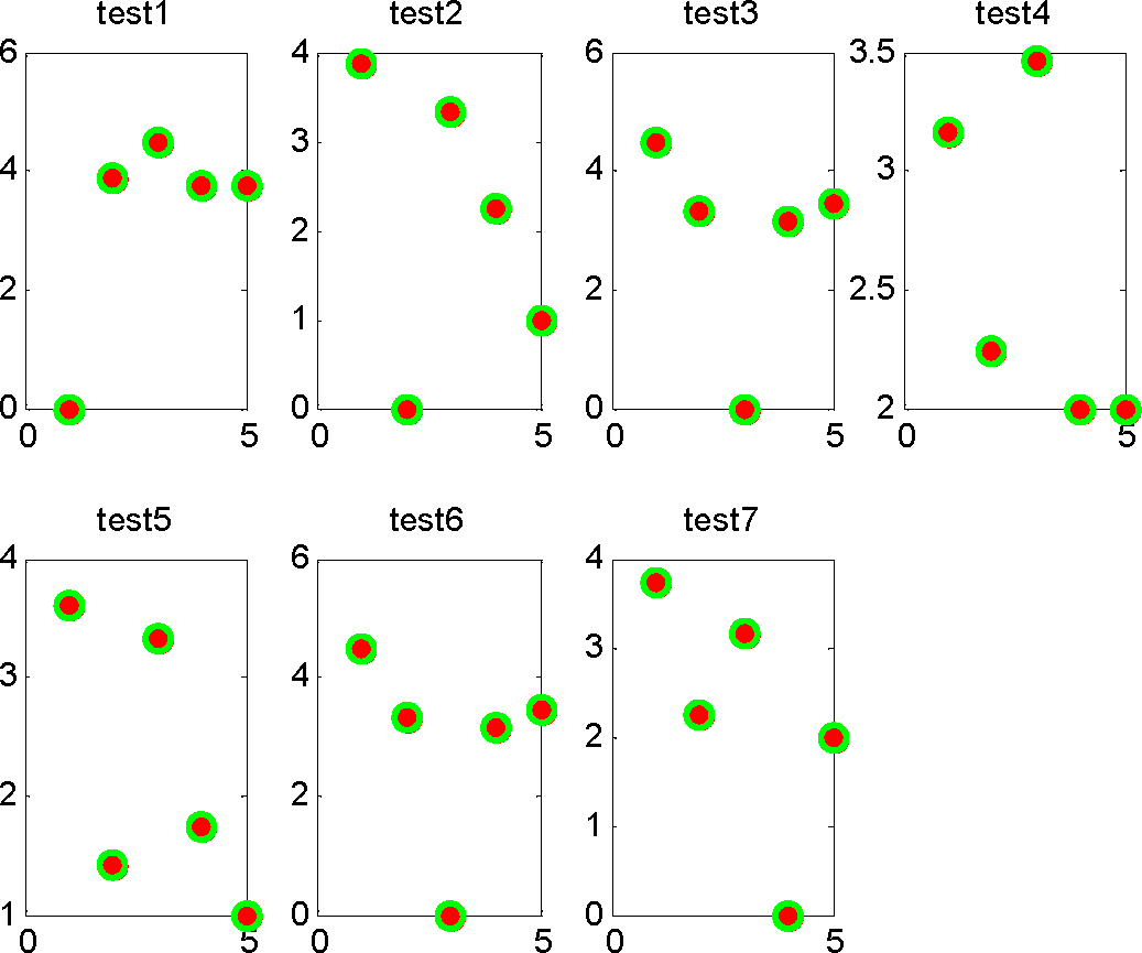
lists the feature vector distances between the seven testing activities and five normal activities, where the first column represents testing activities, columns 2–5 represent the feature vector distances between the testing activity and the five normal activities. Figure 6 is the visualization of the feature vector distances between test sequences 1–7 and normal sequences 1–5. As they show, the distance between testing activities 1–3, 6, 7 and normal activities 1–3, 3, 4 are all equal to zero. Thus, we cannot find the difference between them and judge them as normal activities, despite the fact testing activities 1–3, 6, 7 are abnormal activities. From the table we can see that both normal activities 4 and 5 have minimum distances with testing activity 4, thus we cannot find the most similar normal activity and cannot decide which activity has generated it. For testing activity 5, since there is minimum distance with normal activity 4, we consider normal activity 5 is the most similar to testing activity 5. We compute F_normal = with Equation (13) and get F_normal < 98, thus we consider testing activity 5 is an abnormal activity that was generated by the activity “Clean”.

Obviously, Algorithm 1 not only can recognize abnormal sub-activities of those seven activities quickly, but also can find the type of abnormality, while the feature vector distance-based AAR algorithm can recognize only one of these seven abnormal activities. This is because sequence AAR based on HCRF can capture the sub-structure and context relationships, and thus can distinguish the activities detected by the same sensor with different sensor order and frequency

4.3. Experiment 3

This experiment focuses on the recognition of “new activity” and is also based on the dataset “WSU Apartment Test bed, ADL adlnormal”. In this experiment, we generate another two activities and denote them as activity 6: “From the hall back to the bedroom”, and activity 7: “From the bedroom to the hall”. The two activities have same route, sensor type and sensor number, but have opposite directions, and different order and frequency.

To validate Algorithm 2, we first consider activities 1–5 as training activities and activities 1–7 as testing activities to recognize abnormal activities based on Algorithm 2 and feature vector distance respectively.

For abnormal activities based on Algorithm 2, we first train HCRF with activities 1–5 and compute the likelihood vectors of training activities based on trained HCRF. The MLV and MLV index of activities 1–5 are denoted as (1, 326), (2, 100), (3, 573), (4, 195) and (5, 364). Then, we compute the likelihood vectors of the observation sequences of testing activities 1–7 based on the trained HCRF, respectively. The likelihood vectors of testing activities 1–7 are shown in

Table 5. Likelihood vectors of testing sequences with HCRF.

Testing activities	Likelihood vectors (HCRF, NHS=6)
1	(326.2816, 282.5083, 267.3135, 319.4811, 309.4781)
2	(93.6532, 100.1750, 95.8154, 92.6123, 96.3673)
3	(533.7155, 567.2989, 573.7141, 549.1944, 568.0089)
4	(188.4216, 178.8475, 172.9113, 195.1255, 190.3030)
5	(336.0484, 359.2741, 358.9083, 358.9799, 364.3324)
6	(67.7235, 57.4616, 52.3373, 64.4937, 61.6425)
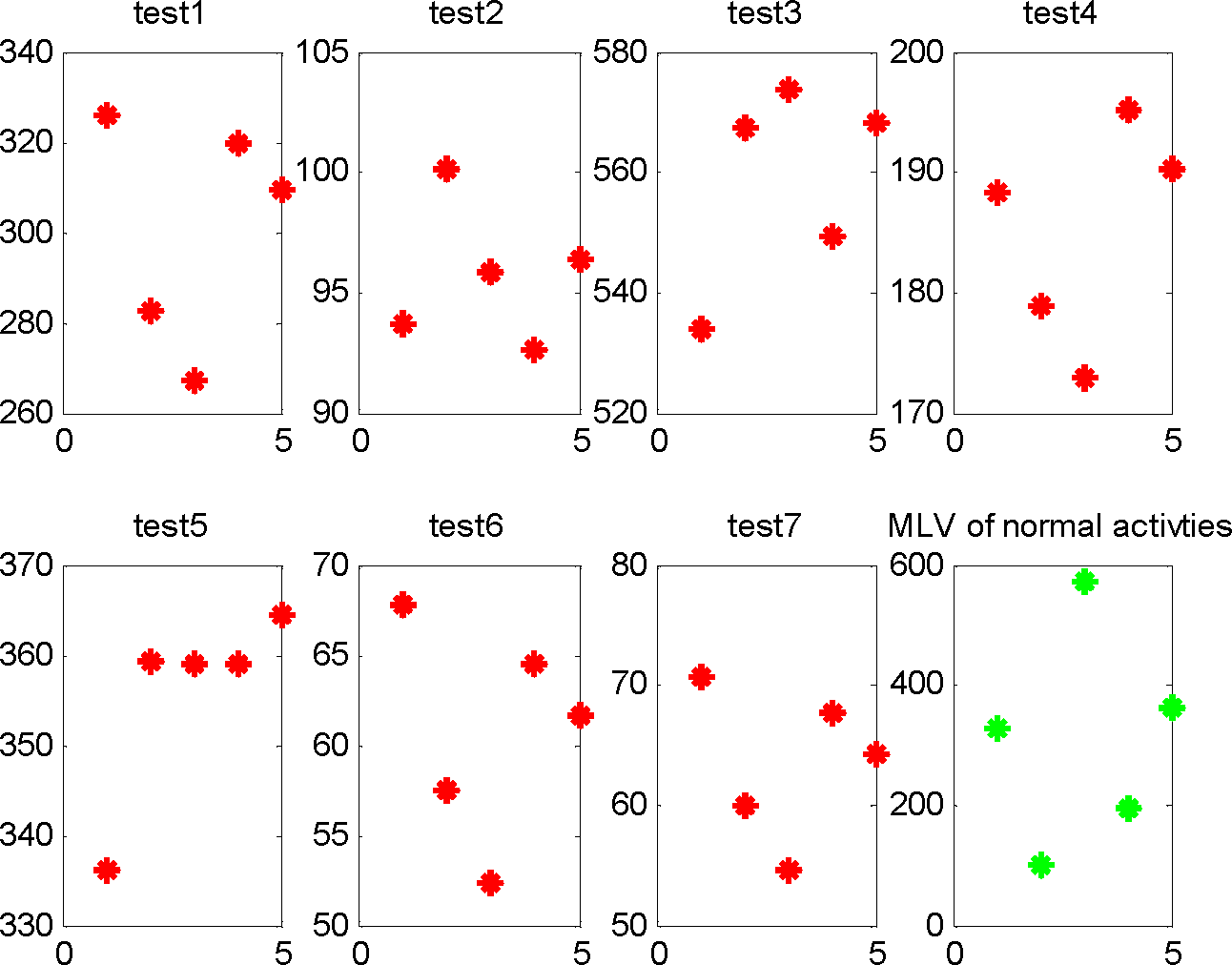
7	(70.7103, 59.9438, 54.5756, 67.7057, 64.3426)

and the visualization of likelihood vectors is shown in Figure 7.

From the table we can see that the MLV of activities 1–5 are 326.2816, 100.1750, 573.7141, 195.1255, 364.3324 and the MLV indexes of activities 1–5 are 1–5. Because their MLV are very close to the MLV of the saved training activities 1–5 and for testing activities 1–5, F_normal < 98, we consider testing activities 1–5 are normal activities. Since the MLV indexes of activities 6, 7 are 1, we compare the MLV 67.7235 and 70.7103 with the MLV of training activity 1 and get F_normal < 98. Thus, we judge activities 6, 7 are rare abnormal activities. In addition to finding abnormalities, our algorithm can also distinguish them as the activities 6, 7 have unequal MLVs.

The feature vector distance-based AAR algorithm first extracts the feature vectors of training activities 1–5 and testing activities 1–7. Then the algorithm computes the feature vector distance between the corresponding training activity and testing activity.

Table 6. Feature vector distances between testing sequences 1–7 and training sequences 1–5.

Testing activities	Feature vector distance
1	0	3.8730	4.4721	3.7417	3.7417
2	3.8730	0	3.3166	2.2361	1.0000
3	4.4721	3.3166	0	3.1623	3.4641
4	3.7417	2.2361	3.1623	0	2.0000
5	3.7417	1.0000	3.4641	2.0000	0
6	1.7321	3.7417	4.3589	3.6056	3.6056
7	1.7321	3.7417	4.3589	3.6056	3.6056

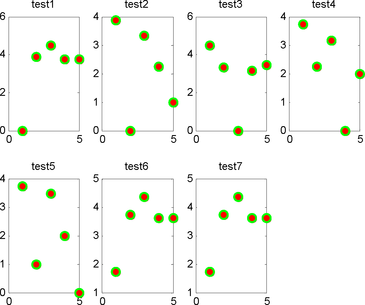
shows the feature vector distances between the testing activities 1–7 and training activities 1–5 and Figure 8 is their visualization.

Because the minimum feature vector distances between testing activities 1–5 and training activities 1–5 are all zero, we consider them as normal activities. Because the testing activities 6, 7 and training activity 1 both have the minimum feature vector distances 1.7321 and F_normal < 98, we consider them as abnormal activities, but because the two testing activities have equivalent minimum feature vector distances with training activity 1, we cannot distinguish them. 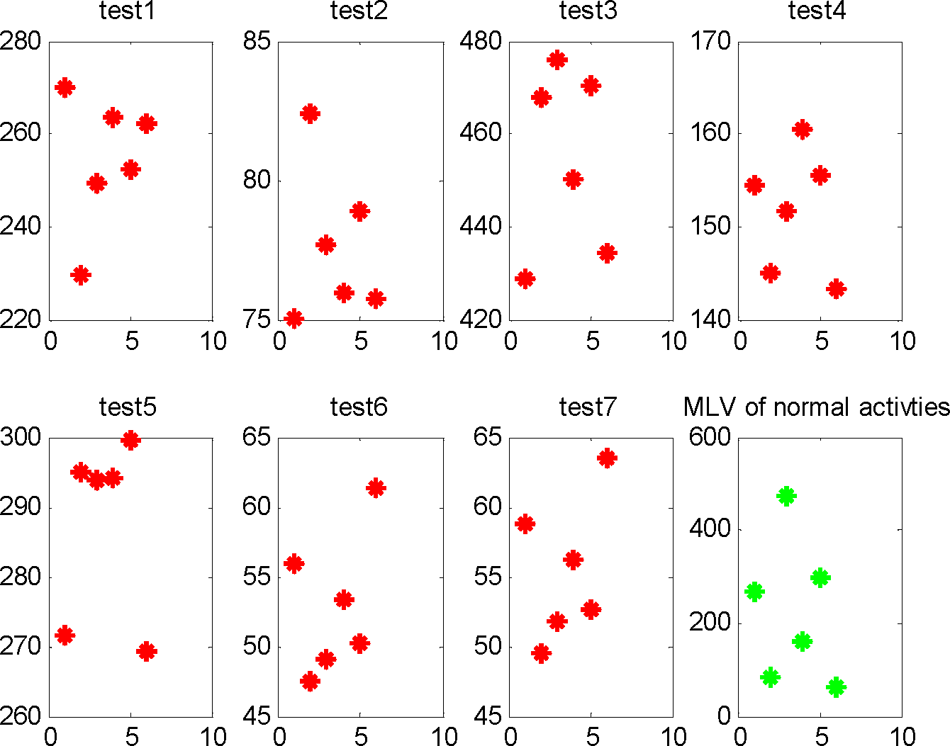To further validate Algorithm 2, we also take activities 1–6 as training activities and activities 1–7 as testing activities, and compare the result with the feature vector distance AAR algorithm. After training HCRF with activities 1–6, we compute the likelihood vectors of training activities based on the trained HCRF.

The MLV and MLV index of training activities 1–6 are denoted as (1, 269), (2, 82), (3, 475), (4, 160), (5, 299) and (6, 61). For testing activities 1–7, we compute the likelihood vectors of the observation sequences based on the trained HCRF, respectively, and the likelihood vectors of testing activities 1–7 are shown in

Table 7. Likelihood vectors of seven testing sequences with HCRF.

Testing activities	Likelihood vectors (HCRF, NHS=6)
1	(269.8225, 229.6156, 249.1611, 263.6643, 252.2116, 262.2444)
2	(75.0678, 82.3581, 77.7119, 75.9655, 78.9250, 75.7699)
3	(428.8811, 467.7071, 475.9057, 450.2416, 470.2999, 434.1561)
4	(154.4092, 145.0172, 151.6422, 160.3794, 155.4553, 143.3504)
5	(271.4594, 295.0582, 293.9657, 294.0288, 299.6182, 269.1849)
6	(55.9792, 47.5435, 49.1397, 53.4108, 50.2745, 61.2882)
7	(58.7701, 49.5426, 51.8330, 56.1844, 52.5862, 63.5533)

and the visualization of likelihood vectors is shown in Figure 9. As the table shows, the MLV of activities 1–7 are 269.8225, 82.358, 475.9057, 160.3794, 299.6182, 61.2882, 63.5533 and the MLV indexes of activities 1–7 are 1–6, 6. For testing activities 1–6, there are F_normal < 98. Thus we consider testing activities 1–6 are normal activities. Since the MLV indexes of activity 7 are 6, we compare the MLV 63.5533 with the MLV 61 of training activity 6 and get F_normal < 98. Thus, we judge activity 7 as a rare abnormal activity.

Similarly, the feature vector distance-based AAR algorithm first extracts the feature vector of training activities 1–6 and testing activities 1–7, and computes the feature vector distance between training activity and testing activity.

Table 8. Feature vector distances between test sequences 1–7 and training sequences 1–6.

Testing activities	Feature vector distance
1	0	3.8730	4.4721	3.7417	3.7417	1.7321
2	3.8730	0	3.3166	2.2361	1.0000	3.7417
3	4.4721	3.3166	0	3.1623	3.4641	4.3589
4	3.7417	2.2361	3.1623	0	2.0000	3.6056
5	3.7417	1.0000	3.4641	2.0000	0	3.6056
6	1.7321	3.7417	4.3589	3.6056	3.6056	0
7	1.7321	3.7417	4.3589	3.6056	3.6056	0

is the feature vector distances between testing activities 1–7 and training activities 1–6. We also give the visualization of the feature vector distances between test sequences and normal sequences in Figure 10. As we know, the activity 7 has not appeared before and is abnormal activity in fact. However, since the minimum feature vector distances between testing activities 1–7 and training activities 1–6 are all zero, we consider them as normal activities. From the assessing of testing activity 7 we can see that feature vector distance based AAR algorithm cannot distinguish activities with same sensor type and sensor number but difference order and frequency.

This experiment shows HCRF can recognize “new activity” and Algorithm 2 not only can distinguish abnormal activities of different sensor types and sensor number well (activities 6 and 7), but also can distinguish abnormal activities with the same sensor type and sensor number but different sensor order and frequency (activity 7).

5. Conclusions

To allow elderly people to be better assisted with context-aware services, this paper introduces the HCRF model-based AAR algorithm for recognizing two types of abnormal activities named “forgetting” and “new activity” which often occur in elderly persons’ homes. To validate the proposed algorithm, in addition to using HCRF to recognize normal activities, the HCRF model-based AAR algorithm as well as feature vector distance-based AAR algorithm is used for comparison in recognizing two types of abnormal activities in two experiments. The results show that the HCRF model-based AAR algorithm outperforms the feature vector distance-based AAR algorithm and confirms that modeling actions (sub-activities) and the underlying correlations can contribute to AAR.

References

1. Augusto, J.C.; McCullagh, P. Ambient intelligence: Concepts and applications. Comput. Sci. Inf. Syst. 2007, 4, 1–26. [Google Scholar]
2. Chen, L.; Nugent, C.D.; Wang, H. A knowledge-driven approach to activity recognition in smart homes. IEEE Trans. Knowl. Data Eng. 2012, 24, 961–974. [Google Scholar]
3. Mahmoud, S.; Lotfi, A.; Langensiepen, C. User activities outliers detection; integration of statistical and computational intelligence techniques. Comput. Intell. 2014. [Google Scholar] [CrossRef]
4. Maglogiannis, I.; Delibasis, K.; Kosmopoulos, D.; Goudas, T.; Doukas, C. Activity recognition in assistive environments: The STHENOS approach. In Universal Access in Human-Computer Interaction. Aging and Assistive Environments; Stephanidis, C., Antona, M., Eds.; Springer International Publishing: New York, NY, USA, 2014; pp. 525–536. [Google Scholar]
5. Zhao, T.; Ni, H.; Zhou, X.; Qiang, L.; Zhang, D.; Yu, Z. Detecting abnormal patterns of daily activities for the elderly living alone. In Health Information Science; Zhang, Y., Yao, G., He, J., Wang, L., Smalheiser, N.R., Yin, X., Eds.; Springer International Publishing: New York, NY, USA, 2014; pp. 95–108. [Google Scholar]
6. Xiang, T.; Gong, S. Video behaviour profiling and abnormality detection without manual labelling, Proceedings of the Tenth IEEE International Conference on Computer Vision, Beijing, China, 17–20 October 2005; IEEE Computer Society: Washington D.C., WA, USA, 2005; pp. 1238–1245.
7. Zhang, X.X.; Liu, H.; Gao, Y.; Hu, D.H. Detecting abnormal events via hierarchical Dirichlet processes. In Advances in Knowledge Discovery and Data Mining; Theeramunkong, T., Kijsirikul, B., Cercone, N., Ho, T.-B., Eds.; Springer: Berlin, Heidelberg, Germany, 2009; pp. 278–289. [Google Scholar]
8. Hu, D.H.; Zhang, X.X.; Yin, J.; Zheng, V.W.; Yang, Q. Abnormal activity recognition based on HDP-HMM models, Proceedings of International Joint Conference on Artificial Intelligence, Pasadena, CA, USA, 11–17 July 2009; Kitano, H., Ed.; Morgan Kaufmann Publishers: San Francisco, CA, USA, 2009; pp. 1715–1720.
9. Yin, J.; Yang, Q.; Pan, J.J. Sensor-based abnormal human-activity detection. IEEE Trans. Knowl. Data Eng. 2008, 20, 1082–1090. [Google Scholar]
10. Hsu, H.H.; Chen, C.C. RFID-based human behavior modeling and anomaly detection for elderly care. Mob. Inf. Syst. 2010, 6, 341–354. [Google Scholar]
11. Hsu, H.H.; Lu, K.C.; Takizawa, M. Abnormal behavior detection with fuzzy clustering for elderly care, Proceedings of 2010 International Computer Symposium, Tainan, Taiwan, 16–18 December 2010; pp. 6–11.
12. Jakkula, V.R.; Cook, D.J. Anomaly detection using temporal data mining in a smart home environment. Methods Inf. Med. 2008, 47, 70–75. [Google Scholar]
13. Jakkula, V.R.; Cook, D.J.; Crandall, A.S. Temporal pattern discovery for anomaly detection in a smart home, Proceedings of 2007 3rd IET International Conference on Intelligent Environments, Ulm, Germany, 24–25 September 2007; pp. 339–345.
14. Jakkula, V.R.; Cook, D.J. Detecting anomalous sensor events in smart home data for enhancing the living experience, Proceedings of Artificial Intelligence and Smarter Living, San Francisco, CA, USA, 7–8 August 2011.
15. Lotfi, A.; Langensiepen, C.; Mahmoud, S.M.; Akhlaghinia, M.J. Smart homes for the elderly dementia sufferers: Identification and prediction of abnormal behaviour. J. Ambient Intell. Humaniz. Comput. 2012, 3, 205–218. [Google Scholar]
16. Wang, C.; Zheng, Q.; Peng, Y.; De, D.; Song, W.-Z. Distributed abnormal activity detection in smart environments. Int. J. Distrib. Sens. Netw. 283197.
17. Mahmoud, S.; Lotfi, A.; Langensiepen, C. Behavioural pattern identification and prediction in intelligent environments. Appl. Soft Comput. 2013, 13, 1813–1822. [Google Scholar]
18. Hsu, K.-C.; Chiang, Y.-T.; Lin, G.-Y.; Lu, C-H.; Hsu, J.Y.-J.; Fu, L.-C. Strategies for inference mechanism of conditional random fields for multiple-resident activity recognition in a smart home. In Trends in Applied Intelligent Systems; García-Pedrajas, N., Herrera, F., Fyfe, C., Benítez, J.M., Ali, M., Eds.; Springer: Berlin, Heidelberg, Germany, 2010; pp. 417–426. [Google Scholar]
19. Nazerfard, E.; Das, B.; Holder, L.B.; Cook, D.J. Conditional random fields for activity recognition in smart environments, Proceedings of the 1st ACM International Health Informatics Symposium, Arlington, VA, USA, 11–12 November 2010; Veinot, T., Ed.; ACM: New York, NY, USA, 2010; pp. 282–286.
20. Vail, D.L.; Veloso, M.M.; Lafferty, J.D. Conditional random fields for activity recognition, Proceedings of the 6th international joint conference on autonomous agents and multiagent systems, Honolulu, HI, USA, 14–18 May 2007; ACM: New York, NY, USA, 2007.
21. Quattoni, A.; Collins, M.; Darrell, T. Conditional random fields for object recognition. Adv. Neural Inf. Process. Syst. 2004, 17, 1097–1104. [Google Scholar]
22. Wang, S.B.; Quattoni, A.; Morency, L; Demirdjian, D.; Darrell, T. Hidden conditional random fields for gesture recognition, Proceedings of 2006 IEEE Computer Society Conference on Computer Vision and Pattern Recognition, New York, NY, USA, 17–22 June 2006; IEEE: New York, NY, USA, 2006; pp. 1521–1527.
23. Lafferty, J.; McCallum, A.; Pereira, F.C. Conditional random fields: Probabilistic models for segmenting and labeling sequence data, Proceedings of the Eighteenth International Conference on Machine Learning, San Francisco, CA, USA, 28 June–1 July 2001; Morgan Kaufmann Publishers: San Francisco, CA, USA, 2001; pp. 282–289.
24. Klinger, R.; Tomanek, K. Classical Probabilistic Models and Conditional Random Fields; Bielefeld University: Bielefeld, Germany, 2007. [Google Scholar]
25. Gong, Y.; Xu, W. Maximum entropy model and conditional random field. Mach. Learn. Multimed. Content Anal. 2008, 30, 201–233. [Google Scholar]
26. Quattoni, A.; Wang, S.; Morency, L.-P.; Collins, M.; Darrell, T. Hidden conditional random fields. IEEE Trans. Pattern Anal. Mach. Intell. 2007, 29, 1848–1852. [Google Scholar]
27. Tong, Y.; Chen, R. Latent-Dynamic conditional random fields for recognizing activities in smart homes. J. Ambient Intell. Smart Environ. 2014, 6, 39–55. [Google Scholar]
28. Pearl, J. Probabilistic Reasoning in Intelligent Systems: Networks of Plausible Inference; Morgan Kaufmann: Burlington, MA, USA, 1988. [Google Scholar]
29. Liu, D.C.; Nocedal, J. On the limited memory BFGS method for large scale optimization. Math. Program. 1989, 45, 503–528. [Google Scholar]
30. Anderson, D.T.; Ros, M.; Keller, J.M.; Cuéllar, M.P.; Popescu, M.; Delgado, M.; Vila, A. Similarity measure for anomaly detection and comparing human behaviors. Int. J. Intell. Syst. 2012, 27, 733–756. [Google Scholar]
31. Quinn, J.A.; Sugiyama, M. A least-squares approach to anomaly detection in static and sequential data. Pattern Recognit. Lett. 2014, 40, 36–40. [Google Scholar]
32. Cook, D.J.; Schmitter-Edgecombe, M. Assessing the quality of activities in a smart environment. Methods Inf. Med. 2009, 48, 480–485. [Google Scholar]
33. Sokolova, M.; Lapalme, G. A systematic analysis of performance measures for classification tasks. Inf. Process. Manag. 2009, 45, 427–437. [Google Scholar]
34. Hsu, C.-W.; Lin, C.-J. A Comparison of Methods for Multiclass Support Vector Machines. IEEE Trans. Neural Netw. 2002, 13, 415–425. [Google Scholar]
35. Zou, B; Peng, Z.-M; Xu, Z.-B. The learning performance of support vector machine classification based on Markov sampling. Sci. China Inf. Sci. 2013, 56, 1–16. [Google Scholar]
Figure 1. (a) Graphical structure of Conditional Random Field. (b) Graphical structure of Hidden Conditional Random Field.
Entropy 17 01358f1
Figure 2. The framework of Abnormal Activity Recognition based on HCRF.
Entropy 17 01358f2
Figure 3. The performing routes of five normal activities (Ai present the i-th activity).
Entropy 17 01358f3
Figure 4. The accuracies of SVM and HCRF model for five individual activities.
Entropy 17 01358f4
Figure 5. The visualization of likelihood vectors of seven testing sequences and MLV of five normal activities.
Entropy 17 01358f5
Figure 6. The visualization of feature vector distances between testing sequences and normal sequences.
Entropy 17 01358f6
Figure 7. The visualization of likelihood vectors of seven testing sequences and MLV of five normal activities.
Entropy 17 01358f7
Figure 8. The visualization of feature vector distances between testing sequences and normal sequences.
Entropy 17 01358f8
Figure 9. The visualization of likelihood vectors of seven testing sequences and MLV of six normal activities.
Entropy 17 01358f9
Figure 10. The visualization of feature vector distances between test sequences and normal sequences.
Entropy 17 01358f10