Entropy Generation Analysis for a CNT Suspension Nanofluid in Plumb Ducts with Peristalsis

Abstract

The purpose of the current investigation was to discuss the entropy generation analysis for a carbon nanotube (CNT) suspension nanofluid in a plumb duct with peristalsis. The entropy generation number due to heat transfer and fluid friction is formulated. The velocity and temperature distributions across the tube are presented along with pressure attributes. Exact analytical solution for velocity and temperature profile are obtained. It is found that the entropy generation number attains high values in the region close to the walls of the tube, while it attains low values near the center of the tube.

1. Introduction

Peristalsis is a series of muscle contractions that occur in your digestive tract. Peristalsis is also seen in some organs that connect the kidneys to the bladder. Peristalsis is an automatic and important process. It moves food through the digestive system, urine from the kidneys into the bladder, bile from the gallbladder into the duodenum. After the first study done by Latham [1], analysis of this process become an interesting topic for researchers, and many theoretical, experimental and numerical studies have been done on this phenomenon [2–8].

Carbon nanotubes (CNTs) are allotropes of carbon with a cylindrical nanostructure. Nanotubes have been constructed with length-to-diameter ratios of up to 132,000,000:1, significantly larger than for any other material. These cylindrical carbon molecules have unusual properties, which are valuable for nanotechnology, electronics, optics and other fields of materials science and technology. In particular, owing to their extraordinary thermal conductivity and mechanical and electrical properties, carbon nanotubes find applications as additives to various structural materials. For instance, nanotubes form a tiny portion of the material(s) in some (primarily carbon fiber) baseball bats, golf clubs, or car parts [9–16].

In thermodynamics, entropy is a measure of the number of specific ways in which a thermodynamic system may be arranged, often taken to be a measure of disorder, or a measure of progress towards thermodynamic equilibrium. Non-Newtonian fluid flow in a pipe system with entropy generation is considered by Pakdemirli and Yilbas [17]. According to them the entropy number increases with increasing Brinkman number. Souidi et al. [18] discussed the entropy generation rate for a peristaltic pump. Entropy generation due to heat and fluid flow in backward facing step flow with various expansion ratios was studied by Abu-Nada [19]. Further analysis can be found [20–24].

Entropy generation for peristaltic flow has not been explored so far, and to fill this gap the author has investigated the analysis of the peristaltic flow of a CNT suspension nanofluid in a plumb duct with entropy generation. The coupled differential equations are simplified under long wavelength and low Reynolds number assumptions. Exact solutions are obtained for the reduced coupled differential equations. The entropy generation is computed by evaluation of the thermal and fluid viscosity contributions. The physical features of pertinent parameters have been discussed by plotting the graphs of velocity, temperature, entropy number and stream functions.

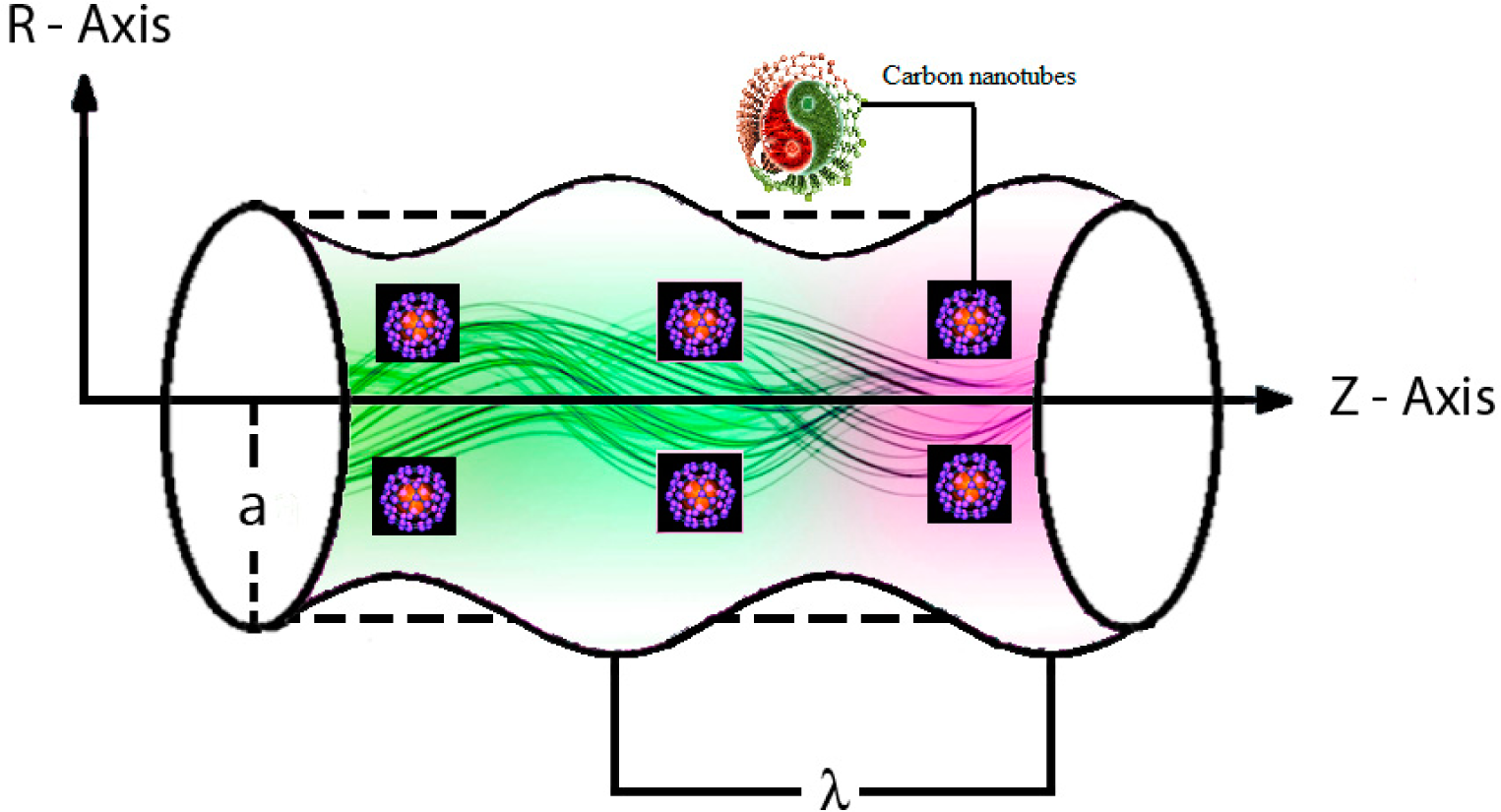
2. Mathematical Formulation

Let us consider the peristaltic flow of an incompressible, peristaltic flow of a CNT suspension nanofluid in a horizontal tube (Figure 1).

A sinusoidal wave is propagating along the walls of the tube. We choose a cylindrical coordinate system $\left(\overline{R},\overline{Z}\right)$(, where the $\overline{Z}$-axis lies along the center line of the tubes and the $\overline{R}$-axis is normal to it. The wave is propagating with a velocity c along the walls of the tube. Keeping in view the analysis geometry of the wall surface it is defined as:

$$\overline{h}=a+b\sin \frac{2\pi }{\lambda }\left(\overline{Z}-c\overline{t}\right).$$

(1)

In the fixed coordinates system $\left(\overline{R},\overline{Z}\right),$ flow between the two tubes is unsteady. It becomes steady in a wave frame $\left(\overline{r},\overline{z}\right)$ moving with the same speed as the wave moves in the $\overline{Z}$ direction. The transformations between the two frames are:

$$\overline{r}=\overline{R},\overline{z}=\overline{Z}-c\overline{t},\overline{v}=\overline{V},\overline{w}=\overline{W}-c,\overline{p}\left(\overline{z},\overline{r},\overline{t}\right)=\overline{p}\left(\overline{Z},\overline{R},\overline{t}\right)$$

(2)

The governing equations for the flow of an incompressible nanofluid can be written as:

$$div\overline{V}=0,$$

(3)

$${\rho }_{nf}\left[\frac{d\overline{V}}{\partial \overline{t}}\right]=-\nabla \overline{p}+{\mu }_{nf}{\nabla }^2\overline{V}-\sigma B_o^2\overline{V},$$

(4)

$${(\rho c)}_{nf}\left[\frac{d\overline{T}}{\partial \overline{t}}\right]=-\nabla \overline{p}+K_{nf}{\nabla }^2\overline{T}+\mathrm{\Phi },$$

(5)

$${\mu }_{nf}\left(2\left({\left(\frac{\partial \overline{u}}{\partial \overline{z}}\right)}^2+{\left(\frac{\partial \overline{w}}{\partial \overline{r}}\right)}^2\right)+{\left(\frac{\partial \overline{u}}{\partial \overline{r}}+\frac{\partial \overline{w}}{\partial \overline{z}}\right)}^2\right).$$

(6)

In component form the above equations can be written as follows:

$$\frac{1}{\overline{r}}\frac{\partial \left(\overline{r}\overline{u}\right)}{\partial \overline{r}}+\frac{\partial \overline{w}}{\partial \overline{z}}=0,$$

(7)

$${\rho }_{nf}\left[\overline{u}\frac{\partial \overline{u}}{\partial \overline{r}}+\overline{w}\frac{\partial \overline{u}}{\partial \overline{r}}\right]=-\frac{\partial \overline{p}}{\partial \overline{r}}+{\mu }_{nf}\frac{\partial }{\partial \overline{r}}\left[2\frac{\partial \overline{u}}{\partial \overline{r}}\right]+{\mu }_{nf}\frac{2}{\overline{r}}\left(\frac{\partial \overline{u}}{\partial \overline{r}}-\frac{\overline{u}}{\overline{r}}\right)+{\mu }_{nf}\frac{\partial }{\partial \overline{z}}\left[\left(\frac{\partial \overline{u}}{\partial \overline{r}}+\frac{\partial \overline{w}}{\partial \overline{z}}\right)\right],$$

(8)

$${\rho }_{nf}\left[\overline{u}\frac{\partial \overline{w}}{\partial \overline{r}}+\overline{w}\frac{\partial \overline{w}}{\partial \overline{z}}\right]=-\frac{\partial \overline{p}}{\partial \overline{z}}+{\mu }_{nf}\frac{\partial }{\partial \overline{z}}\left[2\frac{\partial \overline{w}}{\partial \overline{z}}\right]+{\mu }_{nf}\frac{1}{\overline{r}}\frac{\partial }{\partial \overline{r}}\left[\overline{r}\left(\frac{\partial \overline{u}}{\partial \overline{z}}+\frac{\partial \overline{w}}{\partial \overline{r}}\right)\right]-\sigma B_o^2\left(\overline{w}+c\right),$$

(9)

$${\left({\rho }_{cp}\right)}_{nf}\left(v\frac{\partial \overline{T}}{\partial \overline{r}}+w\frac{\partial \overline{T}}{\partial \overline{z}}\right)=k_{nf}\left[\frac{{\partial }^2\overline{T}}{\partial {\overline{r}}^2}+\frac{1}{\overline{r}}\frac{\partial \overline{T}}{\partial \overline{r}}+\frac{{\partial }^2\overline{T}}{\partial {\overline{z}}^2}\right]+{\mu }_{nf}\left(2\left({\left(\frac{\partial \overline{u}}{\partial \overline{z}}\right)}^2+{\left(\frac{\partial \overline{w}}{\partial \overline{r}}\right)}^2\right)+{\left(\frac{\partial \overline{u}}{\partial \overline{r}}+\frac{\partial \overline{w}}{\partial \overline{z}}\right)}^2\right),$$

(10)

where $\overline{r}$ and $\overline{z}$ are the coordinates. $\overline{z}$ is taken as the center line of the tube and $\overline{r}$ transverse to it, $\overline{u}$ and $\overline{w}$ are the velocity components in the $\overline{r}$ and $\overline{z}$ directions respectively, $\overline{T}$ is the local temperature of the fluid. Further, ρ_nf is the effective density, μ_nf is the effective dynamic viscosity, (ρC_p)_nf is the heat capacitance, α_nf is the effective thermal diffusivity, and k_nf is the effective thermal conductivity of the nanofluid:

$$r=\frac{\overline{r}}{a},z=\frac{\overline{z}}{\lambda },w=\frac{\overline{w}}{c},u=\frac{\lambda \overline{u}}{ac},p=\frac{a^2\overline{p}}{c\lambda {\mu }_f},\delta =\frac{a}{\lambda },\theta =\frac{\left(\overline{T}-{\overline{T}}_0\right)}{{\overline{T}}_0},t=\frac{c\overline{t}}{\lambda },M^2=\frac{\sigma B_0^2{a}^2}{{\mu }_f},B_r=Ec\mathrm{Pr},h=\frac{\overline{h}}{a}.$$

(11)

With the help of Equation (11), Equations (7–10) can be written as follows under the long wave length (δ = 0) and low Reynold’s number Re ≪ 1 assumption:

$$\frac{dp}{dr}=0,$$

(12)

$$\frac{dp}{dz}=\left[\left(\frac{{\mu }_{nf}}{{\mu }_f}\right)\frac{1}{r}\frac{\partial }{\partial r}\left(r\frac{\partial w}{\partial r}\right)-M^2\left(w+1\right)\right],$$

(13)

$$\left(\frac{k_{nf}}{k_f}\right)\frac{1}{r}\frac{\partial }{\partial r}\left(r\frac{\partial \theta }{\partial r}\right)+B_r\left(\frac{{\mu }_{nf}}{{\mu }_f}\right){\left(\frac{\partial w}{\partial r}\right)}^2=0.$$

(14)

The non-dimensionless boundary conditions are defined as follows:

$$\frac{\partial w}{\partial r}=0,\frac{\partial \theta }{\partial r}=0,atr=0,$$

(15a)

$$w=-1,\theta =0,atr=h,$$

(15b)

Thermal properties of the fluid are defined as follows [13–16]:

$$\begin{array}{c}{\rho }_{nf}=\left(1-\phi \right){\rho }_f+\phi {\rho }_f,{\mu }_{nf}=\frac{{\mu }_f}{{\left(1-\phi \right)}^{2.5}},\\ {\left(\rho c_p\right)}_{nf}=\left(1-\phi \right){\left(\rho c_p\right)}_f+\phi {\left(\rho c_p\right)}_s,{\alpha }_{nf}=\frac{k_{nf}}{{\left(\rho c_{k_{CNT}}\right)}_{nf}},\\ k_{nf}=k_f\left(\frac{(1-\phi )+\frac{2\phi k_{CNT}}{k_{CNT}-k_f}\log \left(\frac{k_{CNT}+k_f}{2k_f}\right)}{(1-\phi )+\frac{2\phi k_f}{k_{CNT}-k_f}\log \left(\frac{k_{CNT}+k_f}{2k_f}\right)}\right).\end{array}$$

(16)

3. Viscous Dissipation and Entropy Generation

The dimensional viscous dissipation term $\overline{\mathrm{\Phi }}$ can be obtained from equations of motion, i.e, [17–24]

$$\overline{\mathrm{\Phi }}={\mu }_{nf}\left(2\left({\left(\frac{\partial \overline{u}}{\partial \overline{z}}\right)}^2+{\left(\frac{\partial \overline{w}}{\partial \overline{r}}\right)}^2\right)+{\left(\frac{\partial \overline{u}}{\partial \overline{r}}+\frac{\partial \overline{w}}{\partial \overline{z}}\right)}^2\right),$$

(17)

The dimensional volumetric entropy generation is defined as [17–24].

$$S_{\mathit{gen}}^{″\prime }=\frac{k_{nf}}{{\overline{\theta }}_0^2}\left({\left(\frac{\partial \overline{T}}{\partial \overline{r}}\right)}^2+{\left(\frac{\partial \overline{T}}{\partial \overline{z}}\right)}^2\right)+\frac{\overline{\mathrm{\Phi }}}{{\overline{\theta }}_0},$$

(18)

The dimensionless form of the entropy generation is given as:

$$Ns=\frac{S_{\mathit{gen}}^{″\prime }}{S_G^{″\prime }}=\left(\frac{k_{nf}}{k_f}\right){\left(\frac{\partial \theta }{\partial r}\right)}^2+\mathrm{\Lambda }{B}_r\left(\frac{{\mu }_{nf}}{{\mu }_f}\right){\left(\frac{\partial w}{\partial r}\right)}^2,$$

(19)

where

$$S_G^{″\prime }=\frac{k_f{\overline{T}}_0^2}{{\overline{\theta }}_0^2{a}^2},B_r=\frac{c^2{\mu }_f}{k_f{\overline{T}}_0},\mathrm{\Lambda }=\frac{{\overline{\theta }}_0}{{\overline{T}}_0}.$$

(20)

Equation (19) consists of two parts. The first part is the entropy generation due to finite temperature difference (Nscond) and the second part is the entropy generation due to viscous effects (Nsvisc). The Bejan number is defined as [17–24]

$$\frac{N{s}_{\mathrm{cond}}}{N{s}_{\mathrm{cond}}+N{s}_{\mathrm{visc}}}.$$

(21)

4. Exact Solutions

Exact solutions have been evaluated for velocity, temperature and pressure gradient using the undetermined coefficients method from Equations (12)–(15).

Velocity of the fluid flow is:

$$w\left(r,z\right)=-1-\frac{dp}{dz}\frac{1}{M^2}+\frac{dp}{dz}\frac{I_0\left(Mr\sqrt{{\left(1-\phi \right)}^{2.5}}\right)}{M^2{I}_0\left(hM\sqrt{{\left(1-\phi \right)}^{2.5}}\right)}.$$

(22)

The temperature distribution is given as:

$$\theta \left(r,z\right)=\frac{B_r{\left(\frac{dp}{dz}\right)}^2}{2M^{4}T{I}_0\left(hM\sqrt{T}\right)2}\left(\frac{k_f}{k_{n_f}}\right)\left(\begin{array}{c}{M}^{2}T\left(h^2{I}_1\left(hM\sqrt{T}\right)2-r^2{I}_1\left(Mr\sqrt{T}\right)2\right)\\ +\left(1-h^2{M}^{2}T\right)I_0\left(hM\sqrt{T}\right)2+hM\sqrt{T}{I}_0\left(hM\sqrt{T}\right)I_1\left(hM\sqrt{T}\right)\\ +\left(M^2{r}^{2}T-1\right)I_0\left(Mr\sqrt{T}\right)2-Mr\sqrt{T}{I}_0\left(Mr\sqrt{T}\right)I_1\left(Mr\sqrt{T}\right)\end{array}\right),$$

(23)

where $T=\sqrt{{\left(1-\phi \right)}^{2.5}}.$

Flow rate is given by:

$$F=2\pi \stackrel{h\left(z\right)}{\underset{0}{{\displaystyle \int }}}\mathit{rwdr},$$

this implies that:

$$\frac{dp}{dz}=-\frac{M^2\left(F+\pi h^2\right)I_0\left(hM\sqrt{{\left(1-\phi \right)}^{2.5}}\right)}{\pi h^2{I}_2\left(hM\sqrt{{\left(1-\phi \right)}^{2.5}}\right)},$$

(24)

where the mean flow rate Q is given as:

$$Q=F+\frac{1}{2}\left(1+\frac{{\epsilon }^2}{2}\right).$$

(25)

Integrating Equation (26) over the interval [0,1], we can find the pressure rise given by the expression:

$$\mathrm{\Delta }P=\stackrel{1}{\underset{0}{{\displaystyle \int }}}\frac{dp}{dz}dz.$$

(26)

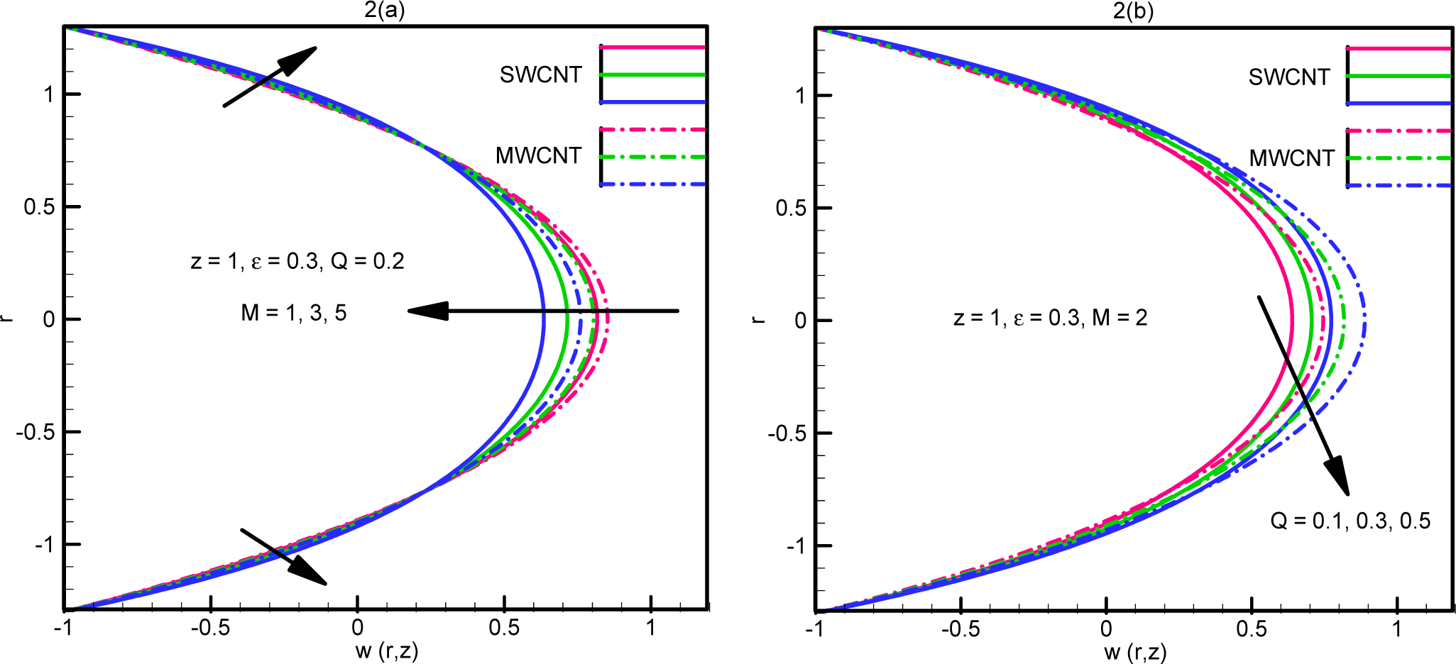
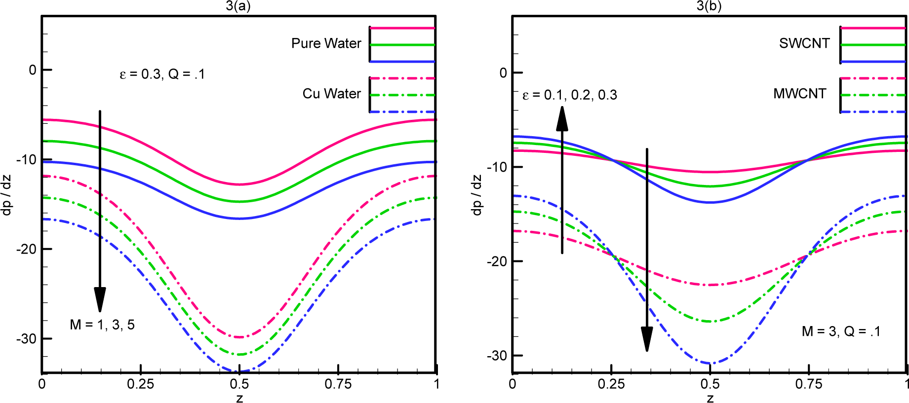
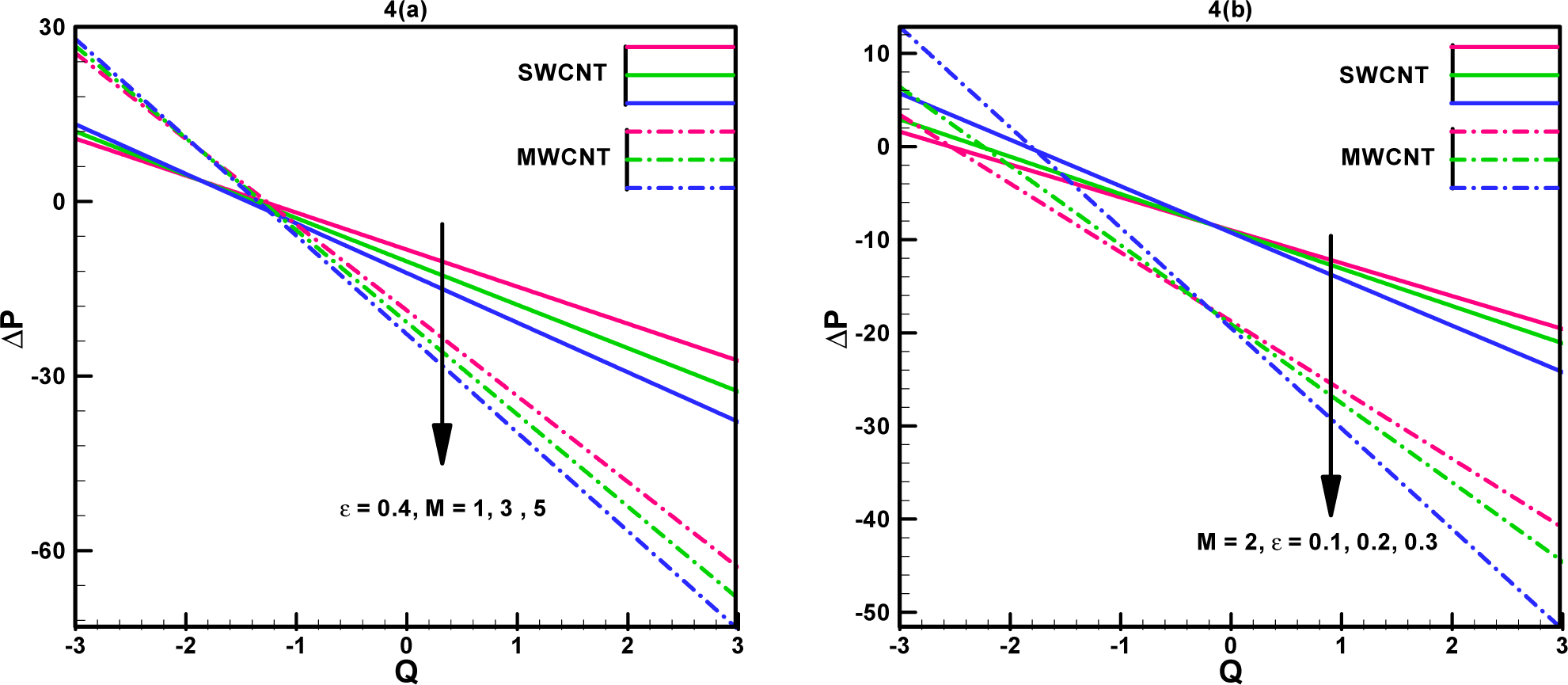
5. Results and Discussion

In this section, we present a brief graphical analysis of the exact analytical solutions of the governing problem. Figure 2 represents the magnitude of the horizontal velocity of the fluid inside the tube. We see that with the increase in the Hartmann number M, i.e., ratio of electromagnetic force to the viscous force, the velocity decreases in the center of the tube and increases near the walls of the tube, while as we increase the flow rate Q, the magnitude of velocity takes a positive shift all around the tube. In both cases, it is observed that MWCNTs have more variation as that of SWCNTd. Also we note that the velocity attains its highest values in the center of the tube at r = 0 while it sufficiently decreases at the walls of the tube. Copper particles, if they are added to CNTs makes the stomach and arteries more flexible and flow can easily move in it.

Figure 3 depicts that with the addition of copper to the base fluid, the pressure gradually decreases. We note that the pressure gradient certainly decreases with a decrease in the Hartmann number. However a non-uniform behavior is seen in case of ε. In that case the pressure gradient seems to be directly proportional to ε for 0 < z < 0.25 and inversely proportional for 0.25 < z <0.75, this behavior of pressure gradient is oscillating. The magnitude of the pressure gradient for MWCNTs is more dominant as compared to SWCNTs.

The pressure rise in the fluid is shown in Figure 4a,b. From the graphical demonstration, it is visible that the pressure rise is directly proportional to M, ε in the peristaltic pumping region and inversely proportional to the same in the augmented peristaltic region. In both cases, the change in case for MWCNTs is observed to be more rapid as compared to SWCNTs.

The temperature of the fluid in the tube increases significantly with an increase in Brinkman number B_r and a decrease in Hartmann number M. However, with less copper in the fluid, the temperature substantially decreases inside the tube. In comparison to the walls of the tube, higher temperature exists in the center where r = 0. We note that with higher values of the Brinkman number, i.e., the ratio of viscous heat generation to external heating, the conduction of heat produced by viscous dissipation will be lesser and hence larger the temperature rise, see Figure 5. The temperature for MWCNTs is observed to be higher as compared to SWCNTs.

Figure 6 was prepared to analyze the entropy generation with respect to changes in the different physical constraints involved. Figure 6a,b depict that entropy generation is directly proportional to both Hartmann number and Brinkman number, and that entropy generation for MWCNTs is higher than that of SWCNTs. It has larger values near the walls of the tube as compared to the center of the tube. It is to be noticed that for significantly larger values of these two parameters, entropy generation can be larger in the center of the tube than at the walls. A similar behavior is seen if we increase the flow rate Q Nevertheless, the higher the values of Λ,ε the smaller the entropy generation. Rapid change in this case is seen in the center of the tube.

Figure 7 is prepared to analyze the Bejan number with respect to changes in the different physical constraints involved. Figure 7 depict that with the increase in Hartmann number, Brinkman number, temperature difference, flow rate and amplitude ratio heat transfer irreversibility is high as compare to the total irreversibility due to heat transfer, fluid friction and magnetic field.

Figure 8 shows streamlines for SWCNTs and MWCNTs. It is seen that the size and number of the trapped bolus for SWCNTs is greater as compared to MWCNTs. Figures 9 and 10 present the streamlines for SWCNTs and MWCNTs with the variation of Hartmann number M It is seen that with the variation of Hartmann number M size and number of trapped bolus for SWCNTs are greater as compared to MWCNTs.

Physical properties for SWCNTs and MWCNTs are presented in

Table 1. Presents the thermal properties of the model.

Physical Properties	Fluid Phase (Water)	SWCNT	MWCNT
cp J/kg K	4719	425	796
ρ kg/m3	997.1	2600	1600
k W/mk	0.613	6600	3000

.

6. Conclusions

Analysis of peristaltic flow of a CNT suspension nanofluid in a plumb duct is investigated. Key points of the performed analysis are as follows:

• With the increase in the Hartmann number the velocity decreases in the center of the tube and increases near the walls of the tube.
• The pressure gradient certainly decreases with a decrease in the Hartmann number.
• Pumping for MWCNTs is observed to be more rapid as compared to SWCNTs.
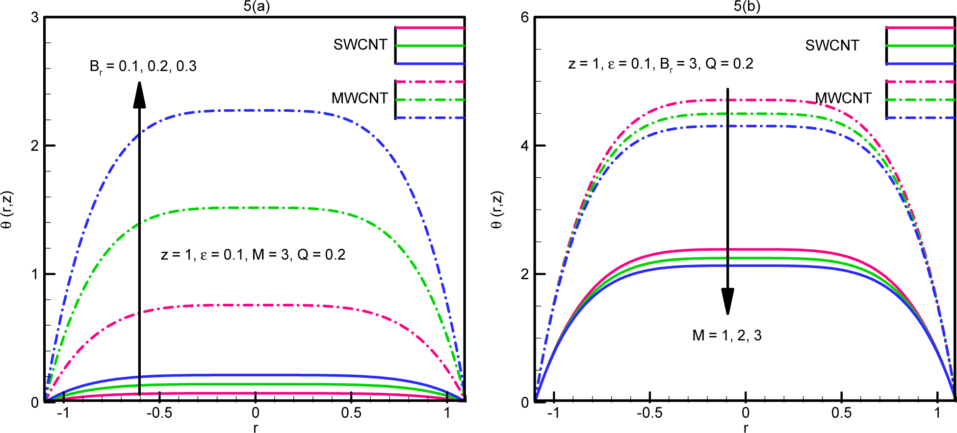
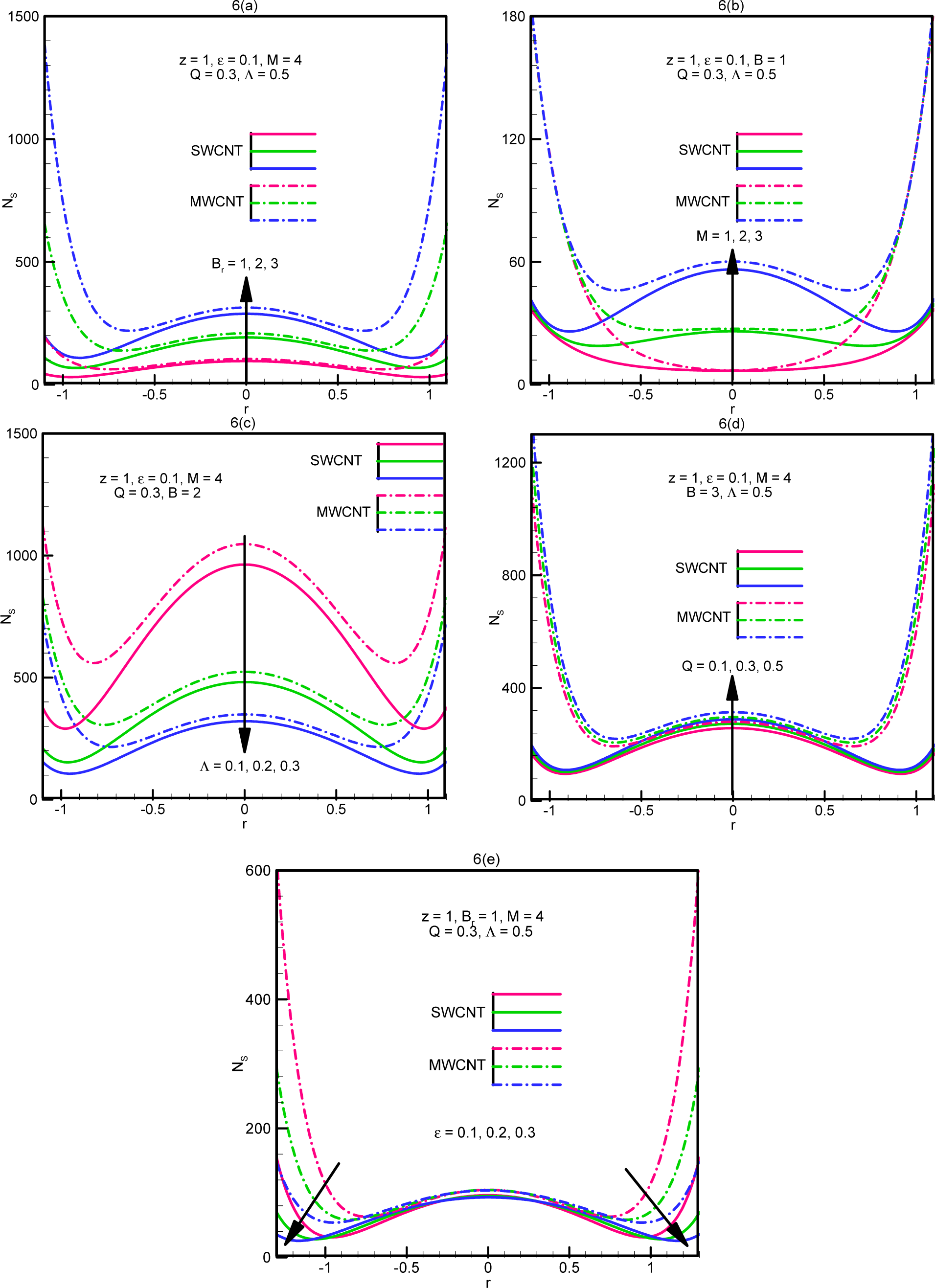
• Entropy generation is directly proportional to both Hartmann number and Brinkman number.
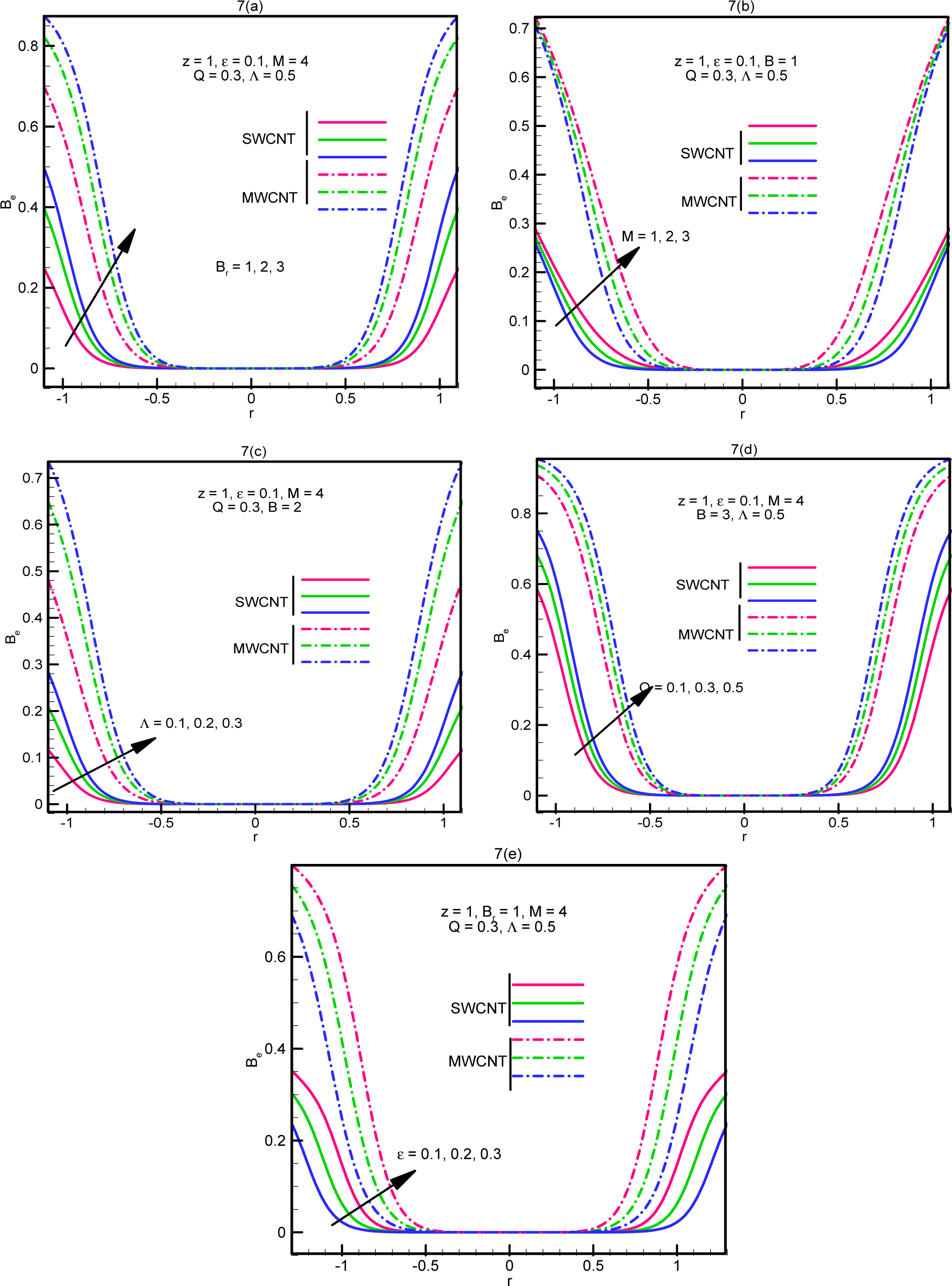
• With the increase in Hartmann number, Brinkman number, temperature difference, flow rate and amplitude ratio heat transfer irreversibility is high as compare to the total irreversibility due to heat transfer, fluid friction and magnetic field.
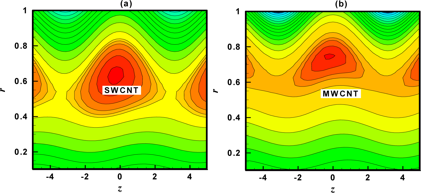
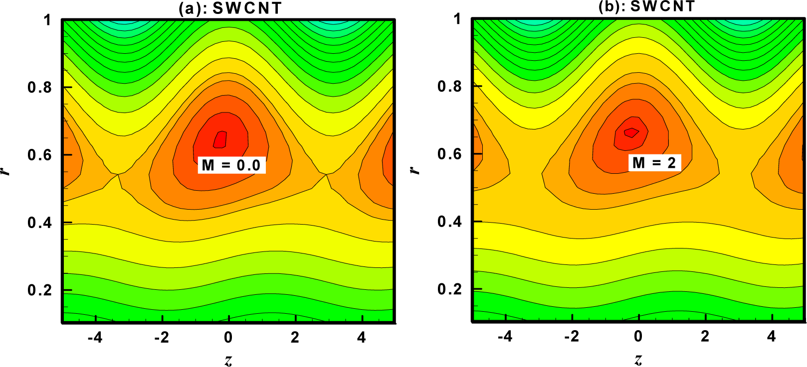
• With the variation of Hartmann number M size and number of trapped bolus for SWCNTs are greater as compared to MWCNTs.

References

1. Latham, T.W. Fluid Motion in a Peristaltic Pump. Master’s Thesis, Massachusetts Institute of Technology, Cambridge, MA, USA, 1965. [Google Scholar]
2. Mekheimer, Kh.S.; Elmaboud, Y.A. The influence of heat transfer and magnetic field on peristaltic transport of a Newtonian fluid in a vertical annulus: Application of an endoscope. Phys. Lett. A 2008, 372, 1657–1665. [Google Scholar]
3. Mekheimer, Kh.S. Effect of the induced magnetic field on peristaltic flow of a couple stress fluid. Phys. Lett. A 2008, 372, 4271–4278. [Google Scholar]
4. Mekheimer, Kh.S.; Salem, A.M.; Zaher, A.Z. Peristatcally induced MHD slip flow in a porous medium due to a surface acoustic wavy wall. J. Egypt. Math. Soc. 2014, 22, 143–151. [Google Scholar]
5. Ellahi, R.; Riaz, A.; Sohail, S.; Mushtaq, M. Series solutions of magnetohydrodynamic peristaltic flow of a Jeffrey fluid in eccentric cylinders. J. Appl. Math. Inf. Sci. 2013, 7, 1441–1449. [Google Scholar]
6. Ellahi, R.; Rahman, S.U.; Nadeem, S. Analytical Solutions of Unsteady Blood Flow of Jeffery Fluid through Stenosed Arteries with Permeable Walls. Zeitschrift Fur Naturforschung A 2013, 68, 489–498. [Google Scholar]
7. Ellahi, R.; Riaz, A.; Sohail, S. Three dimensional peristaltic flow of Williamson in a rectangular duct. Indian J. Phys. 2013, 87, 1275–1281. [Google Scholar]
8. Akbar, N.S. Peristaltic flow of Tangent Hyperbolic fluid with convective boundary condition. Eur. Phys. J. Plus. 2014, 129. [Google Scholar] [CrossRef]
9. Xue, Q.Z. Model for thermal conductivity of carbon nanotube-based composites. Physica B 2005, 368, 302–307. [Google Scholar]
10. Ding, Y.; Alias, H.; Wen, D.; Williams, R.A. Heat transfer of aqueous suspensions of carbon nanotubes (CNT nanofluids). Int. J. Heat Mass Transf. 2006, 49, 240–250. [Google Scholar]
11. Wang, J.; Zhu, J.; Zhang, X.; Chen, Y. Heat transfer and pressure drop of nanofluids containing carbon nanotubes in laminar flows. Exp. Therm. Fluid Sci. 2013, 44, 716–721. [Google Scholar]
12. Meyer, J.; McKrell, T.; Grote, K. The influence of multi-walled carbon nanotubes on single-phase heat transfer and pressure drop characteristics in the transitional flow regime of smooth tubes. Int. J. Heat Mass Transf. 2013, 58, 597–609. [Google Scholar]
13. Akbar, N.S.; Nadeem, S.; Khan, Z.H. Thermal and velocity slip effects on the MHD peristaltic flow with carbon nanotubes in an asymmetric channel: Application of radiation therapy. Appl. NanoSci. 2014, 4, 849–857. [Google Scholar]
14. Akbar, N.S. MHD peristaltic flow with carbon nanotubes in an asymmetric channel. J. Comput. Theor. Nanosci. 2014, 11, 1323–1329. [Google Scholar]
15. Akbar, N.S. Peristaltic flow with Maxwell carbon nanotubes suspensions. J. Comput. Theor. Nanosci. 2014, 11, 1642–1648. [Google Scholar]
16. Akbar, N.S.; Nadeem, S.; Khan, Z.H. The combined effects of slip and convective boundary conditions on stagnation-point flow of CNT suspended nanofluid over a stretching sheet. J. Mol. Liq. 2014, 196, 21–25. [Google Scholar]
17. Pakdemirli, M.; Yilbas, B.S. Entropy generation in a pipe due to Non-Newtonian fluid flow: Constant viscosity case. Sadhana 2006, 31, 21–29. [Google Scholar]
18. Souidi, F.; Ayachi, K.; Benyahia, N. Entropy generation rate for a peristaltic pump. J. Non-Equilib. Thermodyn 2009, 34, 171–194. [Google Scholar]
19. Abu-Nada, E. Entropy generation due to heat and fluid flow in backward facing step flow with various expansion ratios. Int. J. Exergy. 2006, 3, 419–435. [Google Scholar]
20. Yilbas, B.S.; Yürüsoy, M.; Pakdemirli, M. Entropy analysis for Non-Newtonian fluid flow in annular pipe: Constant viscosity case. Entropy 2004, 6, 304–315. [Google Scholar]
21. Hassan, M.; Sadri, R.; Ahmadi, G.; Dahari, M.B.; Kazi, S.N.; Safaei, M.R.; Sadeghinezhad, E. Numerical study of entropy generation in a flowing nanofluid used in micro- and minichannels. Entropy 2013, 15, 144–155. [Google Scholar]
22. Bouabid, M.; Magherbi, M.; Hidouri, N.; Rahim, A.B. Entropy generation at natural convection in an inclined rectangular cavity. Entropy 2011, 13, 1020–1033. [Google Scholar]
23. Bianco, V.; Manca, O.; Nardini, S. Entropy generation analysis of turbulent convection flow of Al2O3-water nanofluid in a circular tube subjected to constant wall heat flux. Energy Convers. Manag. 2014, 77, 306–314. [Google Scholar]
24. Burg, B.R.; Schneider, J.; Bianco, V.; Schirmer, N.C.; Poulikakos, D. Selective parallel integration of individual metallic single-walled carbon nanotubes from heterogeneous solutions. Langmuir 2010, 26, 10419–10424. [Google Scholar]
Figure 1. Geometry of the problem.
Entropy 17 01411f1
Figure 2. Velocity profile w(r,z) against the radial distance r.
Entropy 17 01411f2
Figure 3. Pressure gradient d p d z versus z.
Entropy 17 01411f3
Figure 4. Pressure rise ΔP against the flow rate Q.
Entropy 17 01411f4
Figure 5. Temperature profile θ(r,z).
Entropy 17 01411f5
Figure 6. Entropy NS against the radial distance r.
Entropy 17 01411f6
Figure 7. Variation of Bejan number Be against the radial distance r.
Entropy 17 01411f7
Figure 8. Streamlines for: (a) SWCNTs; (b) MWCNTs.
Entropy 17 01411f8
Figure 9. Streamlines for SWCNTs with the variation of Hartmann number M.
Entropy 17 01411f9
Figure 10. Streamlines for MWCNTs with the variation of Hartmann number M.
Entropy 17 01411f10