A Comparison of Nonlinear Measures for the Detection of Cardiac Autonomic Neuropathy from Heart Rate Variability

Abstract

In this work we compare three multiscale measures for their ability to discriminate between participants having cardiac autonomic neuropathy (CAN) and aged controls. CAN is a disease that involves nerve damage leading to an abnormal control of heart rate, so one would expect disease progression to manifest in changes to heart rate variability (HRV). We applied multiscale entropy (MSE), multi fractal detrended fluctuation analysis (MFDFA), and Renyi entropy (RE) to recorded datasets of RR intervals. The latter measure provided the best separation (lowest p-value in Mann–Whitney tests) between classes of participants having CAN, early CAN or no CAN (controls). This comparison suggests the efficacy of RE as a measure for diagnosis of CAN and its progression, when compared to the other multiscale measures.

1. Introduction

Cardiac rhythm is controlled by the membrane properties of the sino-atrial node, neuro-hormonal and autonomic nervous system (ANS) modulation [1,2]. CAN is a disease often presenting as a complication of diabetes, which affects ANS modulation of the heartbeat. 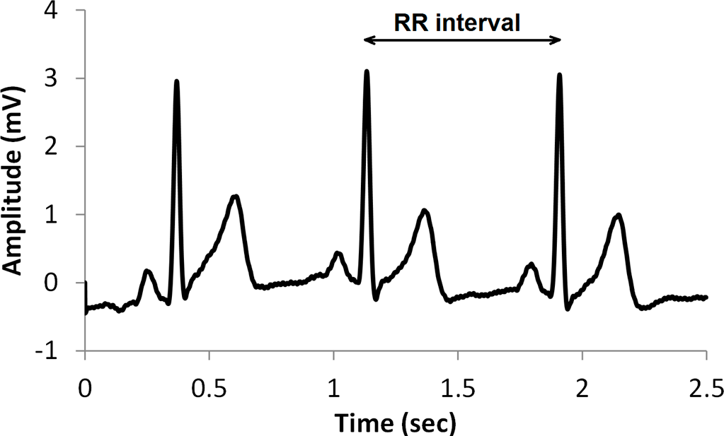CAN is characterised by peripheral nerve damage leading to abnormal regulation of the heartbeat by the ANS [3,4] and may manifest in up to 60% of individuals with type 2 diabetes at different stages during diabetes disease progression [5]. One would therefore expect such a condition to be characterised by changes in HRV, which describes the beat to beat (or RR interval) changes and is not concerned with the full details of the electrocardiogram (ECG).

A typical ECG signal is illustrated in Figure 1, and the RR interval is shown as the time between successive beats. The letters PQRST are commonly used to identify ECG features. The fiducial point or peak of the QRS wave can be identified most easily. Therefore this is used to obtain an RR interval tachogram from which HRV can be obtained. The natural rhythm of the human heart is known to vary in response to sympathetic and parasympathetic signals. Generally, sympathetic activity decreases the RR intervals and decreases variability, whereas parasympathetic activity increases the RR intervals and increases variability [6]. HRV is a useful indication of the health of the cardiovascular system, and is commonly used in assessing the regulation of cardiac autonomic function [7,8]. A variety of measures can be extracted from the RR interval time series, ranging from time series measures, through frequency domain measures to more complex non-linear measures [9–11]. All of these can be derived from the RR interval time series through suitable mathematical functions. Some examples of time domain measures are the standard deviation of the RR intervals obtained from the normal beats of a time series (SDNN), and the number of pairs of successive intervals that differ by more than 50 ms divided by the total number of intervals (pNN50%). Frequency-domain methods divide the spectral distribution into very low, low and high frequency regions. Low frequency (LF) power is believed to be indicative of both parasympathetic and sympathetic activity. High frequency (HF) is indicative of parasympathetic activity. Very low frequency (VLF) is a sensitive indicator of management of metabolic processes and reflects deficit energy states [12].

Examples of nonlinear measures include fractal and entropy measures. It is this group of measures which are examined in this work. In spite of a growing literature illustrating their use in HRV analysis, there is a shortage of empirical comparisons between different nonlinear/multiscale methods, particularly in relation to CAN and CAN progression. We examine how changing the value of scaling, length and parameters of the fractal and entropy algorithms provides a family of measures, and forms a multiscale series. The results of the different permutations of the multiscale measures are compared in terms of distinguishing CAN from controls in participants attending the diabetes complications screening clinic in Albury, Australia.

Multi-scale measures are those that provide a series of measures as a function of some scaling factor. The idea of multi-scale used in this paper requires some explanation. Not all of the measures considered here are multi-scale in the same sense. MSE examines RR intervals at a number of different scales in order to provide multiple measures based on the same time series. MFDFA and RE are multi-scale in the sense that a parameter is used to control the order or power that a quantity is raised to. This can take multiple values and so provides multiple measures. Previous work has compared several entropy measures in terms of their efficacy in distinguishing congestive heart failure and arrhythmia from normal sinus rhythm [13]. However in this work we aim to compare two commonly applied multiscale entropy measures and MFDFA, and focus on a single morbidity, CAN, in its early and later stages in asymptomatic individuals with no cardiovascular disease or diabetes.

2. Methods

The aim of this work is to determine which, out of a variety of available multi-scale measures, is most suitable for detecting CAN, and to elucidate the reasons for the discriminatory power, or lack thereof, manifested by these methods. The work reported here used data from the Charles Sturt Diabetes Complications Screening Group (DiScRi), Australia [14]. The study was approved by the Charles Sturt University Human Ethics Committee and written informed consent was obtained from all participants. All recordings were obtained in a temperature stable environment following a 5–10 min rest period in a supine position by all participants. The sampling rate was set to 400 samples/s and recordings pre-processed according to the method described in Tarvainen [15]. A 20-min lead II ECG recording was taken from participants attending the clinic, using a Maclab Pro with Chart 7 software (ADInstruments, Sydney, Australia). Participants were comparable for age, gender, and heart rate, and after initial screening, those with heart disease, presence of a pacemaker, kidney disease or polypharmacy (including multiple anti-arrhythmic medication) were excluded from the study. The same conditions were used for each participant. The status of CAN was defined using the Ewing battery criteria [11,16,17], and each participant was assigned as either without CAN (71 participants), early CAN (67 participants) or definite CAN (11 participants). From the 20-min recording, a 15-min segment was selected from the middle in order to remove start up artefacts and movement at the end of the recording. From this shorter recording, the RR intervals were extracted. No other information was used in this study. The RR interval series for each participant was detrended and the measures used were determined from these data [3].

2.1. Multi-Scale Sample Entropy

The entropy H(X) of an RR interval time series {x₁, …, x_n} expresses the uncertainty of the n intervals as a random variable X, where:

$$H\left(X\right)=-{\displaystyle \sum }_{i=1}^{n}p\left(x_i\right)\log p\left(x_i\right)$$

(1)

The probability p_i may be estimated from the RR interval data by discretising the range of values for X and dividing the number of times that X falls within its discretising band by n. This is the histogram method. Sample entropy generalises this to consider a sequence of m RR intervals X_m(i) = {x_i, …, x_i+m−1} and estimates a probability for X_m(i). However, the histogram method rapidly becomes impractical as the sequence length m is increased, so the probability may be estimated by counting instead the number of sequences which are similar when their elements x_i are compared and the difference is less than a threshold r. The number of sequences c_m(i) are counted having length m and starting at j (j ≠ i) X_m(j) where each scalar comparison |xi − xj| ≤ r. The total number of sequences of length m across the entire series is given by:

$$c_m={\displaystyle \sum }_{i=1}^{n-m+1}{c}_m\left(i\right).$$

(2)

The sample entropy can be seen as the probability that a sequence of RR intervals of length m that repeats itself within a threshold r, will also repeat itself if the sequence length is extended to m + 1. Sample entropy calculates the negative logarithm of the ratio of two measures A and B:

$$SampEn=-\mathit{log}\frac{A}{B},$$

(3)

where B = c_m is the number of matches from sequences of RR intervals of length m and A = c_m+1 is a similar measure calculated using sequences of length m + 1 [18]. MSE extends this concept by using coarse grained copies of the original data series:

$$y_j^{(\tau )}=\frac{1}{\tau }{\displaystyle \sum }_{i=\left(j-1\right)\tau +1}^{j\tau }{x}_i,$$

(4)

where τ is the scale factor and 1 ≤ j ≤ n/τ, and the x_i of Equation (2) is replaced by y_j, so that MSE is a function of the scale [18–20]. The implementation used in this work was from PhysioNet [21].

2.2. Multi-Fractal Detrended Fluctuation Analysis

MFDFA is based on DFA, a fractal-like measure that examines the self-similarity properties of a time series, in this case a sequence of RR intervals. In the ensuing discussion, we follow the implementation of [22], providing here a summary of that work translated from Matlab code into a series of equations, for the convenience of the reader. The Matlab code is available online [23]. Given a sequence of RR intervals {x₁, …, x_n} this is transformed into a random walk by subtracting the mean and calculating the cumulative sum:

$$X_k={\displaystyle \sum }_{i=1}^k\left(x_i-\stackrel{-}{x}\right).$$

(5)

The transformed series X is divided into sequences of length s and a straight line is fitted to each sequence by minimising the sum of the squared errors, to provide a slope and offset. It is possible to use higher order polynomials to fit the segments, but in the work we always use a linear fit. The rms error of the fit ε_ν is calculated for each segment ν of length m:

$${\epsilon }_{\nu }=\sqrt{{\displaystyle \sum }_{i=m\nu }^{m(\nu +1)}{\left(X_i-{\stackrel{\prime }{X}}_l\right)}^2},$$

(6)

where $\acute{X_i}$ is the estimated value of X_i. The mean root mean square (rms) error is found for all segments of length m:

$${\epsilon }_m=\sqrt{\frac{1}{n/m}{\displaystyle \sum }_{\nu =1}^{n/m}{\epsilon }_{\nu }{}^2.}$$

(7)

As with the normal techniques for estimation of fractal dimension, these data are visualized as a graph where the values of ε_m are plotted against m, using a logarithmic scale for both axes, and the slope of the resulting curve is calculated. This slope is the value of DFA.

In order to derive a multifractal measure, Equation (3) is modified by substituting an exponent q that can be varied as a parameter of the method:

$${\epsilon }_{q,m}={\left(\frac{1}{n/m}{\displaystyle \sum }_{\nu =1}^{n/m}{\epsilon }_{\nu }{}^q\right)}^{1/q},$$

(8)

where n/m is the number of segments in the complete series of length m.

2.3. Renyi Entropy

RE is naturally a multi-scale measure, as it generalizes the Shannon entropy and includes the Shannon entropy as a special case [24]. The efficacy of RE for discriminating stages of AN impairments in different scales has been demonstrated [25]. RE is defined as:

$$H\left(\alpha \right)=\frac{1}{1-\alpha }{\log }_2\left({\displaystyle \sum }_{i=1}^n{p}_i^{\alpha }\right),$$

(9)

where p_i is the probability that a random variable takes a given value out of n values, and α is the exponent or order of the entropy measure. When α is varied this provides the multi-scale measure. H(0) is simply the logarithm of n. As α increases the measures become more sensitive to the values occurring at higher probability and less to those occurring at lower probability, which provides a picture of the RR length distribution within a signal. However, the entropy requires an estimate of probabilities, and there are a number of ways in which this can be determined. In previous work, we have described two main methods of estimating probabilities: the histogram method and the density method [26]. In that work we showed that the density method is superior in terms of providing a measure that can discriminate different classes of CAN, without simply duplicating linear measures such as the standard deviation of the RR intervals.

The density method estimates the probability of a sequence of RR intervals of length m using a notional density of space around a point, representing the sequence embedded in an m-dimensional space. This can be done by comparing other RR intervals in the vicinity of the individual RR sequence using a distance measure and considering the two sequences to be similar if each element is less than a threshold. For example, the calculation of sample entropy described above counts all RR intervals that are closer to the individual RR interval given a specific threshold r. However this depends on choosing a suitable value for the threshold. Alternatively, a Gaussian kernel is centred on the individual RR interval and all RR intervals are added, weighted by the Gaussian function, based on the distance between the individual RR interval and the other RR intervals. The extension to the Gaussian kernel method is the density measure, which can be calculated for the individual RR interval with index i, as the sum of all contributions from other RR intervals with index j:

$${\rho }_i=\frac{1}{\sigma \sqrt{2\pi }}{\displaystyle \sum }_{i=1}^n{e}^{-\frac{dis{t}_{\mathit{ij}}^2}{2{\sigma }^2}},$$

(10)

using a distance measure:

$$dis{t}_{\mathit{ij}}^2={\displaystyle \sum }_{k=1}^m{(x_{i+k}-x_{j+k})}^2,$$

(11)

where σ is the dispersion of the function and replaces the threshold r. This provides a continuous rather than a discretised measure.

The MSE was calculated using the default parameters of sequence length m = 2, threshold r = 0.15, and coarse graining factor 1 to 10. As the recordings are only 15 min in length, this restricts the length of sequence m and the scale of coarse graining τ. Note that when τ = 1, the measure is equivalent to the sample entropy without multi scaling. MFDFA was calculated using integer values of order from −5 to +5. A range of scaling exponents similar to MFDFA, α from −5 to +5 was used to determine RE. The RE was then calculated using sequence length m = 16 and σ = 0.16 (see above). For each measure, A Mann–Whitney test was performed to compare the Normal to the Early group, the Early to the Definite group, and the Definite to the Normal group.

3. Results and Discussion

Development of algorithms to characterize HRV of healthy and unhealthy subjects has been an ongoing endeavor, especially with relation to nonlinear methods as standard measures such as SDNN can lead to incorrect interpretation of pathology [27,28]. The proposal of nonlinear methods to address the nonlinearity and non-stationarity as well as complexity of HR time signals as led to the introduction several methods of which MSE, MFDFA and the multiscale RE have been extensively applied. However whether these algorithms have similar or different sensitivities in classifying pathology has not been investigated. In previous studies we have shown that there is a loss of HRV with progression of CAN, which may be related to continued increases in blood sugar levels [29–31].

Results from the Mann–Whitney test using linear measures of HRV time and frequency domain analysis are shown in

Table 1. Results of Mann–Whitney test for comparison between different classes of participants using time and frequency domain measures. All results are significant at the p < 0.05 level. Comparisons shown are Normal vs. Early, Early vs. Definite, and Definite vs. Normal.

Scale	SDNN	pNN50%	LF power (ms2)	HF power (ms2)
N vs. E	0.000	0.002	0.000	0.001
E vs. D	0.011	0.002	0.017	0.024
D vs.N	0.000	0.000	0.000	0.000

. These will be used to put in context the results from the multiscale methods. The heading row lists the measure used. The lower three rows in the table report p-values obtained from the Mann–Whitney test. The first row corresponds to a comparison of normal and early CAN, (N vs. E). The second row contains results of early CAN vs. definite CAN (E vs. D), and the third row definite CAN vs. normal (D vs. N). These results are all below 0.05, so suggest the separation of these classes is possible using any one of these measures. However, these measures will be further assessed by using receiver operating characteristic (ROC) analysis, as this draws attention not only to the separation of classes, but also to the effect of false positives and false negatives.

Results from ROC analysis for time and frequency domain HRV measures are shown in

Table 2. Area under the ROC curve for comparison between different classes of participants using common time and frequency domain measures. Results > 0.8 are shown in bold face. Comparisons shown are normal vs. early, early vs. definite, and definite vs. normal.

Scale	SDNN	pNN50%	LF power (ms2)	HF power (ms2)
N vs. E	0.302	0.352	0.282	0.334
E vs. D	0.261	0.237	0.275	0.287
D vs.N	0.869	0.891	0.888	0.837

. Here a value of 0.5 implies that there is no discriminating power, while a value of 1 is the maximum. The entries in the Table having a value above 0.8 all correspond to the comparison between definite and normal classes of participants. These results suggest that these standard measures are able to distinguish these two classes but not to reliably distinguish early CAN from either normal or definite CAN.

Summary statistics for the MSE are shown in

Table 3. Summary statistics for different classes of participants (N—Normal, E—Early and D—Definite) using MSE. Headings in the row designated as “scale” provide the number of RR intervals used to derive the measure. Values are provided for the upper quartile, median, and lower quartile.

	Scale	1	2	3	4	5	6	7	8	9	10
N	Upper	2.018	2.069	2.011	1.918	1.922	1.846	1.813	1.709	1.642	1.569
	Median	1.855	1.983	1.889	1.791	1.764	1.648	1.631	1.519	1.439	1.339
	Lower	1.700	1.770	1.610	1.621	1.513	1.428	1.352	1.277	1.199	1.066
E	Upper	2.068	2.128	2.035	1.961	1.937	1.930	1.902	1.781	1.722	1.625
	Median	1.953	1.972	1.872	1.827	1.758	1.812	1.682	1.598	1.531	1.437
	Lower	1.815	1.855	1.753	1.588	1.617	1.584	1.477	1.426	1.337	1.190
D	Upper	2.140	2.137	2.129	2.015	2.066	2.018	1.805	1.761	1.767	1.762
	Median	1.929	1.928	1.904	1.762	1.706	1.748	1.645	1.659	1.581	1.551
	Lower	1.610	1.737	1.636	1.504	1.668	1.441	1.516	1.242	1.199	1.154

. The heading row contains the scales used in the analysis, and range from 1 to 10 RR intervals. There are rows for the upper quartile, median and lower quartile, and groups are labelled as N for normal, E for early CAN, and D for definite, according to the result of the Ewing tests. Of note is the relatively large inter-quartile range of participants in the definite group, compared to other groups. The median value for each group is similar for most of the scales, with some exceptions. The median for the normal group, using a scale of 1 (one RR interval) is low compared to other groups (1.855 compared to 1.953 or 1.929). The median for the normal group using a scale of 6 or 8 is also low compared to the other groups.

Results from the Mann–Whitney test are shown in

Table 4. Results of test for comparison between different classes of participants using MSE. Results at the p < 0.05 level are shown in bold face. Comparisons shown are Normal vs. Early, Early vs. Definite, and Definite vs. Normal. Of interest is also that none of the scale factors for MSE distinguished between normal and definite CAN as was the case for the linear HRV measures. This suggests the linear and nonlinear contributions to the tachograms may vary with disease progression.

Scale	1	2	3	4	5	6	7	8	9	10
N vs. E	0.035	0.361	0.376	0.450	0.369	0.028	0.143	0.032	0.083	0.156
E vs. D	0.746	0.509	0.872	0.782	0.936	0.819	0.647	0.652	0.882	0.661
D vs.N	0.661	0.812	0.665	0.976	0.740	0.420	0.749	0.455	0.307	0.270

. Only three results are significant at the p < 0.05 level, and these are all for normal vs. early comparisons, using a sequence lengths of one (equivalent to the sample entropy), six and eight RR intervals. These significant results reflect the differences in median observed in Table 3 and discussed above. The low number of significant results cast doubt upon the sensitivity of this method to indicate any useful discrimination of CAN even for larger data sets.

Results from ROC analysis are shown in

Table 5. Area under the ROC curve for comparison between different classes of participants using MSE. Results > 0.6 are shown in bold face. Comparisons shown are Normal vs. Early, Early vs. Definite, and Definite vs. Normal.

Scale	1	2	3	4	5	6	7	8	9	10
N vs. E	0.602	0.545	0.543	0.537	0.544	0.606	0.571	0.604	0.584	0.569
E vs. D	0.529	0.559	0.515	0.525	0.507	0.520	0.542	0.540	0.513	0.540
D vs. N	0.538	0.522	0.538	0.502	0.530	0.572	0.529	0.567	0.592	0.599

. Only three entries in the Table have a value above 0.6 and these are exactly the same entries as those with p < 0.05 in Table 4. These results offer little evidence that MSE is able to discriminate classes of participants.

Summary statistics for MFDFA are shown in

Table 6. Summary statistics for different classes of participants (N—Normal, E—Early and D—Definite) using MFDFA. Headings in the row labelled “q-order” denote the exponent used in Equation (8). Values are provided for the upper quartile, Median, and lower quartile.

	q-order	−5	−4	−3	−2	−1	0	+1	+2	+3	+4	+5
N	Upper	0.081	0.081	0.084	0.091	0.119	0.191	0.294	0.353	0.381	0.390	0.396
	Median	0.040	0.043	0.047	0.062	0.103	0.166	0.234	0.272	0.291	0.285	0.289
	Lower	0.010	0.016	0.027	0.046	0.086	0.140	0.186	0.209	0.215	0.218	0.218
E	Upper	0.130	0.129	0.120	0.121	0.132	0.207	0.303	0.376	0.402	0.403	0.401
	Median	0.073	0.074	0.078	0.081	0.112	0.176	0.258	0.303	0.293	0.302	0.295
	Lower	0.025	0.029	0.037	0.054	0.088	0.135	0.199	0.243	0.240	0.231	0.217
D	Upper	0.181	0.179	0.171	0.148	0.142	0.213	0.330	0.402	0.435	0.441	0.448
	Median	0.132	0.132	0.130	0.128	0.122	0.184	0.257	0.316	0.336	0.339	0.335
	Lower	0.053	0.057	0.063	0.071	0.109	0.143	0.180	0.206	0.209	0.165	0.130

. The heading row contains the values of q from Equation (8), varying from −5 to +5 [22]. There are rows for the upper quartile, median and lower quartile, and groups are labelled as N for Normal, E for Early CAN, and D for Definite, according to the result of the Ewing tests. For positive values of q the medians are similar between the different classes and most are close to 0.3. For negative values of q, values of MFDFA are largest for Definite CAN and smallest for Normal, suggesting that these measures may be able to differentiate between the different classes.

Table 7. Results of Mann–Whitney test for comparison between different classes of participants using MFDFA variables calculated from RR interval series. Results at the p < 0.05 level are shown in bold face. Comparisons shown are Normal vs. Early, Early vs. Definite, and Definite vs. Normal.

q-order	−5	−4	−3	−2	−1	0	+1	+2	+3	+4	+5
N vs. E	0.065	0.018	0.004	0.011	0.108	0.282	0.141	0.068	0.156	0.375	0.500
E vs. D	0.281	0.201	0.118	0.080	0.196	0.618	0.777	0.861	1.000	0.957	0.989
D vs. N	0.054	0.019	0.004	0.001	0.014	0.296	0.302	0.342	0.553	0.585	0.695

shows the results of the Mann–Whitney test on values obtained using MFDFA. Significant results at the p < 0.05 level were obtained for most of the negative values of q, for comparison between Normal and Early, and between Definite and Normal classes of participants, but not for any of the comparisons between Early and Definite CAN. This suggests that this method is able to distinguish CAN from controls, and even recognize those in the Early class as having CAN. The consistent nature of the low p-values for a range of values of parameter q suggests that this approach is able to yield results that are useful in discrimination of both early and definite CAN from Normal (controls).

Of interest is the observation that measures most successful in discriminating classes were all from the negative side of the spectrum. Examining Table 7 shows that not a single measure using a positive value for q was able to achieve p < 0.05. The best result was for q = −2, providing p < 0.001 for D vs N. Comparing this with the measure using q = +2, we observe that the latter is related to the standard deviation of rms errors involved in fitting straight line segments across all sequences in a single time series of RR intervals. Conversely, the measure using q = −2 is related to the standard deviation of the reciprocal of rms errors, while the measure for q = −3 is related to the kurtosis of the reciprocal of rms errors. The relative success of the measures for negative q suggests that the transformation involved in the inverse, maps these values of rms error into a space where disease classes are more distinct.

Results from ROC analysis are shown in

Table 8. Area under the ROC curve for comparison between different classes of participants using MFDFA variables calculated from RR interval series. Results > 0.7 are shown in bold face. Comparisons shown are Normal vs. Early, Early vs. Definite, and Definite vs. Normal.

q-order	−5	−4	−3	−2	−1	0	+1	+2	+3	+4	+5
N vs. E	0.589	0.614	0.640	0.622	0.577	0.552	0.571	0.588	0.568	0.543	0.532
E vs. D	0.598	0.616	0.642	0.659	0.618	0.545	0.526	0.516	0.500	0.505	0.501
D vs. N	0.673	0.710	0.762	0.797	0.720	0.594	0.593	0.585	0.553	0.549	0.535

. These results support the conclusion that negative values of q are more useful than positive values. Consistent with the results of the Mann–Whitney test in Table 7, these results suggest that the most easily distinguished classes are Definite and Normal. The results presented in Table 8 are larger than those for the linear measures of Table 5, approaching 0.8 for q of −3 and −2. AUC values greater than 0.8 can be considered to have clinical significance, so some of the results shown here are promising. Also, several of the tests comparing Early CAN with other classes provided results above 0.6, suggesting detection of Early CAN. It should be noted that the AUC is equivalent to the Mann–Whitney U-statistic: the figures used in Table 7 are p-values, whereas the figures used in Table 8 are comparable to the value of the Mann–Whitney U-statistic. In addition, the equivalence is subject to a number of assumptions, including the independence of samples, the distribution of false positives (FPs) being Gaussian, and similar variance of the two samples [32].

Results for RE, based on probabilities calculated using the density method, are shown in

Table 9. Summary statistics for different classes of participants (N—Normal, E—Early and D—Definite) using RE. Headings in the row labelled “exponent” denote α as used in Equation (9). Values are provided for the upper quartile, Median, and lower quartile.

	Exponent	−5	−4	−3	−2	−1	+1	+2	+3	+4	+5
N	Upper	1.230	1.202	1.163	1.107	1.038	0.998	0.996	0.995	0.994	0.993
	Median	1.087	1.063	1.043	1.021	1.007	0.998	0.992	0.989	0.986	0.985
	Lower	1.032	1.023	1.013	1.005	1.001	0.997	0.983	0.977	0.972	0.969
E	Upper	1.138	1.109	1.072	1.034	1.008	0.998	0.997	0.997	0.996	0.996
	Median	1.031	1.021	1.012	1.005	1.001	0.998	0.996	0.995	0.994	0.993
	Lower	1.005	1.003	1.001	1.000	0.999	0.997	0.993	0.991	0.989	0.988
D	Upper	1.105	1.082	1.052	1.020	1.003	0.998	0.998	0.997	0.997	0.997
	Median	1.002	1.001	1.000	0.999	0.999	0.998	0.997	0.997	0.997	0.996
	Lower	1.000	0.999	0.999	0.998	0.998	0.998	0.996	0.996	0.995	0.995

. The heading row contains the values of the exponent parameter α used in Equation (9), which varies from −5 to +5. The results for α = 0 are not shown because, due to normalization, the entropy calculated using this value always results in unity. Because all values of RE calculated in this way are close to 1, it is difficult to discern any pattern from these data. However, notice that for negative values of α, RE is greater for Normal and smaller for Definite, and for positive values of α the opposite is true.

Table 10. Results of Mann–Whitney test for comparison between different classes of participants using RE variables calculated from RR interval series. Results at the p < 0.05 level are shown in bold face. Comparisons shown are Normal vs. Early, Early vs. Definite, and Definite vs. Normal.

Exponent	−5	−4	−3	−2	−1	+1	+2	+3	+4	+5
N vs. E	0.001	0.001	0.001	0.001	0.000	0.000	0.000	0.000	0.000	0.000
E vs. D	0.063	0.059	0.061	0.051	0.036	0.056	0.038	0.041	0.037	0.034
D vs. N	0.001	0.001	0.001	0.001	0.000	0.000	0.000	0.000	0.000	0.000

shows the result on the Mann–Whitney tests for RE. All of the comparisons made between Normal and Early, and between Definite and Normal, were significant at the p ≤ 0.001 level. Also, a good number of those for the comparison of Early to Definite were significant, more so for positive values of the exponent α parameter. RE results are also more consistent across groups, with results associated with a negative exponent α parameter decreasing with disease progression and vice versa. The difference between negative and positive values for the exponent α has been explored in our previous work [26]. In that work, we showed that although positive values of α provide higher discrimination of classes, with corresponding lower p-values, the entropy values resulting from positive exponents were highly correlated with the standard deviation. While the standard deviation is a useful measure of HRV, it falls into the category of linear measures of HRV discussed above, and is correspondingly simpler to calculate than RE. The standard deviation has also been shown to be less discriminatory for disease condition [28]. Therefore RE based on positive values of α is of less interest. The measures based on negative values of α are more interesting since they clearly discriminate between classes, but may provide information complimentary to that derived from time domain measures such as the standard deviation.

Results from ROC analysis are shown in

Table 11. Area under the ROC curve for comparison between different classes of participants using RE variables calculated from RR interval series. Results > 0.7 are shown in bold. Comparisons shown are Normal vs. Early, Early vs. Definite, and Definite vs. Normal.

Exponent	−5	−4	−3	−2	−1	+1	+2	+3	+4	+5
N vs. E	0.657	0.658	0.660	0.667	0.685	0.705	0.715	0.720	0.721	0.723
E vs. D	0.669	0.672	0.670	0.678	0.691	0.674	0.689	0.686	0.690	0.692
D vs. N	0.792	0.794	0.798	0.801	0.821	0.828	0.847	0.854	0.859	0.862

. All values calculated for the Disease vs. Normal test show AUC greater than, or close to 0.8, indicating clinical significance. Results comparing Early CAN with the other classes show promise in discriminating the early stages of CAN (r² = 0.723). RE appears to be useful for discriminating the Early class from the others, although values calculated using positive values of α appear to show better separation. The use of RE based on negative values of α, in conjunction with the standard deviation, would therefore be indicated as a powerful test for Early CAN. Thus a combination of HRV measures to discriminate between CAN subtypes and CAN progression may provide useful clinical information as it includes results from both linear and nonlinear measures [33,34].

4. Conclusions

Traditional HRV analysis is based on the assumptions of linearity, stationary and equilibrium nature of heart rate time signals. Nonlinear and multiscale studies applying MSE, MFDFA and RE have indicated a high level of complexity in HRV dynamics based on the observation of a power law relationship when viewing the power spectral density for varying time scales. Hence traditional HRV analysis using time and frequency domain are often not sufficient to characterize the complex dynamics inherent in the heart rate time series [25,28,35]. However, this work is not intended as a definitive comparison between traditional and multiscale measures, and in no way diminishes the usefulness of the former. In previous work, we compared RE with classical measures based on the time domain and frequency domain of single RR intervals [33,34,36]. In that work we showed the efficacy of the RE as a complimentary measure that can extend and enhance the information that may be gleaned from sequences of RR intervals characterized by time and frequency analysis. In this work we show that RE has superior discriminatory power to MSE and MFDFA.

Multiscale measures of HRV have generated a great deal of interest but a systematic approach is required in order to identify appropriate measures that may be of benefit in the context early identification of disease is of clinical importance to the practitioner. In this work we compared three approaches that yield multiscale measures, and evaluated their potential for discriminating different classes of CAN. We found that MSE afforded no useful discrimination between disease categories. In contrast, MFDFA provided a set of measures that were clearly able to discriminate these classes, but only when using negative values of the parameter q, that is, the inverse of the rms errors arising from fitting straight line segments to sequences of RR intervals. This suggests a transformation that can be applied in the calculation of MFDFA, which maps data into a new space of rms error values where these measures are more coherent, in the sense of disease groups occupying similar space. This is an important outcome, although further work is required to fully articulate the implications of this finding.

Using RE we were able to demonstrate a very strong separation of disease classes across all values of the parameter α, showing a very robust measure that can be used to identify CAN, especially early CAN, where treatment intervention is most effective. This conclusion is supported by low p-values obtained from the nonparametric Mann–Whitney test, and by results from ROC analysis. The physiological meaning of the measures such as these is not currently clear. Entropy in general is known to quantify the randomness of a system, and the RE measure H(1) is equivalent to the Shannon entropy, but it should also be noted that in this paper RE was calculated for sequences of 16, rather than single RR intervals, which complicates interpretation. For our dataset the choice of 16 beat sequences was optimal and suggests that this is an important time scale, which reflects the period of possible nonlinear oscillations involved in the pathophysiology of CAN progression [37]. What can be said, therefore, is that sequences of this length measured by RE can carry information of both sympathetic and parasympathetic functions of the autonomic system. In doing so, the value of α chosen will of necessity be sensitive to different aspects of sympathovagal balance, which may reflect changes in the baroreflex responsiveness due to CAN progression. Further, the decrease in entropy for negative values of α may reflect the loss of nonlinear dynamics naturally inherent as part of the cardiac rhythm and therefore loss of capacity of the heart to respond to different physiological demands [38]. Although participants were comparable for age, gender, and heart rate, they were not fully matched and this may be a limitation of this study.