Information-Theoretic Inference of Common Ancestors

Abstract

A directed acyclic graph (DAG) partially represents the conditional independence structure among observations of a system if the local Markov condition holds, that is if every variable is independent of its non-descendants given its parents. In general, there is a whole class of DAGs that represents a given set of conditional independence relations. We are interested in properties of this class that can be derived from observations of a subsystem only. To this end, we prove an information-theoretic inequality that allows for the inference of common ancestors of observed parts in any DAG representing some unknown larger system. More explicitly, we show that a large amount of dependence in terms of mutual information among the observations implies the existence of a common ancestor that distributes this information. Within the causal interpretation of DAGs, our result can be seen as a quantitative extension of Reichenbach’s principle of common cause to more than two variables. Our conclusions are valid also for non-probabilistic observations, such as binary strings, since we state the proof for an axiomatized notion of “mutual information” that includes the stochastic as well as the algorithmic version.

1. Introduction

Causal relations among components X₁,…, X_n of a system are commonly modeled in terms of a directed acyclic graph (DAG) in which there is an edge X_i → X_j whenever X_i is a direct cause of X_j. Further, it is usually assumed that information about the causal structure can be obtained through interventions in the system. However, there are situations in which interventions are not feasible (too expensive, unethical or physically impossible) and one faces the problem of inferring causal relations from observational data only. To this end, postulates linking observations to the underlying causal structure have been employed, one of the most fundamental being the causal Markov condition [1,2]. It connects the underlying causal structure to conditional independencies among the observations. Explicitly, it states that every observation is independent of its non-effects given its direct causes. It formalizes the intuition that the only relevant components of a system for a given observation are its direct causes.

In terms of DAGs, the causal Markov condition states that a DAG can only be a valid causal model of a system if every node is independent of its non-descendants given its parents. The graph is then said to fulfill the local Markov condition [3]. Consider for example the causal hypothesis X → Y←Z on three observations X, Y and Z. Assuming the causal Markov condition, the hypothesis implies that X and Z are independent. The violation of this independence then allows one to exclude this causal hypothesis. However, note that in general, there are many DAGs that fulfill the local Markov condition with respect to a given set of conditional independence relations. For example, all three DAGs X → Y → Z, X←Y → Z and X←Y←Z encode that X is independent of Z given Y, and this cannot be decided from information on conditional independences alone, which is the true causal model. Nevertheless, properties that are shared by all valid DAGs (e.g., an edge between X and Y in the example) provide information about the underlying causal structure.

The causal Markov condition is only expected to hold for a given set of observations if all relevant components of a system have been observed, that is if there are no confounders (causes of at least two observations that have not been measured). It can then be proven by assuming a functional model of causality [1,4,5]. As an example, consider the observations X₁,…, X_n to be jointly distributed random variables. In this case, the causal Markov condition can be derived for a given DAG on X₁,…, X_n from two assumptions: (1) every variable X_i is a deterministic function of its parents and an independent (possibly unobserved) noise variable N_i, and (2) the noise variables N_i are jointly independent. However, in this paper, we assume that our observations provide only partial knowledge about a system and ask for structural properties common to all DAGs that represent the independencies of some larger set of elements.

To motivate our result, assume first that our observation consists of only two jointly-distributed random variables X₁ and X₂, which are stochastically dependent. Reichenbach [6] postulated already in 1956 that the dependence of X₁ and X₂ needs to be explained by (at least) one of the following cases: X₁ is a cause of X₂, or X₂ is a cause of X₁, or there exists a common cause of X₁ and X₂. This link between dependence and the underlying causal structure is known as Reichenbach’s principle of common cause. It is easily seen that by assuming X₁ and X₂ to be part of some unknown larger system whose causal structure is described by a DAG G, then the causal Markov condition for G implies the principle of common cause. Moreover, we can subsume all three cases of the principle if we formally allow a node to be an ancestor of itself and arrive at:

The common cause principle: If two observations X₁ and X₂ are dependent, then they must have a common ancestor in any DAG modeling some possibly larger system.

Our main result is an information-theoretic inequality that enables us to generalize this principle to more than two variables. It leads to the:

Extended common cause principle (informal version): Consider n observations X₁,…, X_n, and a number c, 1≤c≤n. If the dependence of the observations exceeds a bound that depends on c, then in any DAG modeling some possibly larger system, there exist c nodes out of X₁,…, X_n that have a common ancestor.

Thus, structural information can be obtained by exploiting the degree of dependence on the subsystem, and we would like to emphasize that, in contrast to the original common cause principle, the above criterion provides a means to distinguish among cases with the same independence structure of the observed variables. This is illustrated in Figure 1.

Above, the extended common cause principle is stated without making explicit the kind of observations we consider and how dependence is quantified. In the main case we have in mind, the observations are jointly-distributed random variables, and dependence is quantified by the mutual information [7] function. Then the extended common cause principle (Theorem 2) relates stochastic dependence to a property of all Bayesian networks that include the observations.

However, the result holds for more general observations (such as binary strings) and for more general notions of mutual information (such as algorithmic mutual information [8]). Therefore, we introduce an “axiomatized” version of mutual information in the following section and describe how it can be connected to a DAG. Then, in Section 3, we prove a theorem on the decomposition of information about subsets of a DAG out of which the extended common cause principle then follows as a corollary. Apart from a larger area of applicability, we think that an abstract proof based on an axiomatized notion of information better illustrates that the result is independent of the notion of “probability”. It only relies on the basic properties of (stochastic) mutual information (see Definition 1). Finally, in Section 4, we describe the result in more detail within different contexts and relate it to the notion of redundancy and synergy that was introduced in the area of neural information processing.

2. General Mutual Information and DAGs

Before introducing a general notion of mutual information, let us describe how it is connected to a DAG in the stochastic setting. Assume we are given an observation of n discrete random variables X₁,…, X_n in terms of their joint probability distribution p(X₁,…, X_n). Write [n] = f1,…, ng, and for a subset S⊆ [n], let X_S be the random variable associated with the tuple (X_i)_i2S. Assume further that a directed acyclic graph (DAG) G is associated with the nodes X₁,…, X_n that fulfill the local Markov condition [3]: for all i, (1 ≤ i ≤ n):

$$X_i╨X_{n{d}_i}|X_{p{a}_i},$$

(1)

where nd_i and pa_i denote the subset of indices corresponding to the non-descendants and to the parents of X_i in G. The tuple (G, p(X_[n])) is called a Bayesian net [9] and the conditional independence relations imply the factorization of the joint probability distribution

$$p\left(x_1,\dots ,x_n\right)={\displaystyle \prod _{i\in [n]}p}\left(x_i|x_{p{a}_i}\right),$$

where small letters x_i stand for values of the random variables X_i. From this factorization, it follows that the joint information measured in terms of Shannon entropy [7] decomposes into a sum of individual conditional entropies:

$$H(X_1,\dots ,X_n)={\displaystyle \sum _{i=1}^{n}H(X_i|X_{p{a}_i})}.$$

(2)

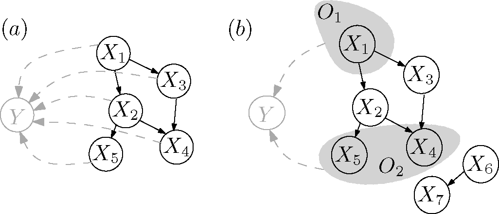
Shannon entropy can be considered as the absolute measure of information. However, in many cases, only a notion of information relative to another observation may be available. For example, in the case of continuous random variables, Shannon entropy can be negative, and hence, may not be a good measure of the information. Therefore, we would like formulate our results based on a relative measure, such as mutual information, which, moreover, induces a notion of independence in a natural way. This can be achieved by introducing a specially-designated variable Y relative to which information will be quantified. The variable Y can, for example, be thought of as providing a noisy measurement of the X_[n] (Figure 2a). Then, with respect to a joint probability distribution p(Y, X_[n]), we can transform the decomposition of entropies into a decomposition of mutual information [7]:

$$I(Y:X_{[n]})\ge {\displaystyle \sum _{i=1}^{n}I(Y:X_i|X_{p{a}_i})}.$$

(3)

For a proof and a condition for equality, see Lemma 2 below. In the case of discrete variables, Shannon entropy H(X_i) can be seen as mutual information of X_i and a copy of itself: H(X_i) = I(X_i : X_i). Therefore, we can always choose p(Y|X_[n]), such that Y = X_[n] and the decomposition of entropies in (2) is recovered. We are interested in decompositions as in (2) and (3), since their violation allows us to exclude possible DAG structures.

However, note that the above relations are not yet very useful, since they require, through the assumption of the local Markov condition, that we have observed all relevant variables of a system. Before we relax this assumption in the next section, we introduce mutual information measures on general observations.

Definition 1 (Measure of mutual information). Given a finite set of elements$\mathcal{O}$, a measure of mutual information on$\mathcal{O}$ is a three-argument function on the power set:

$$I:2^{\mathcal{O}}\times 2^{\mathcal{O}}\times 2^{\mathcal{O}}\to ℝ,\left(A,B,C\right)\to I\left(A:B|C\right)$$

such that, for disjoint sets A, B, C, D ⊆ $\mathcal{O}$, it holds:

$$\begin{array}{l}I(A:\varnothing )=0\left(normalization\right)\\ I\left(A:B|C\right)\ge 0(non-negativity)\\ I\left(A:B|C\right)=I\left(B:A|C\right)(symmetry)\\ I\left(A:\left(B\cup C\right)|D\right)=I\left(A:B|C\cup D\right)+I\left(A:C|D\right)\left(chainrule\right).\end{array}$$

We say A is independent of B given C and write (A ╨ B |C) iff I(A : B |C) = 0. Further, we will generally omit the empty set as a third argument and substitute the union by a comma, hence, we write I(A : B) instead of I(A : B |∅) and I(A : B, C) instead of I(A : B ∪ C).

Of course, mutual information of discrete, as well as of continuous random variables is included in the above definition. Further, in Section 4.2, we will discuss a recently-developed theory of causal inference [4] based on the algorithmic mutual information of binary strings [10]. We now state two properties of mutual information that we need later on.

Lemma 1 (Properties of mutual information). Let I be a measure of mutual information on a set of elements$\mathcal{O}$. Then:

• (Data processing inequality) For three disjoint sets A, B, C ⊆ $\mathcal{O}$:

  $$I\left(A:C|B\right)=0\Rightarrow I\left(A:B\right)\ge I\left(A:C\right).$$
• (Increase through conditioning on independent sets) For three disjoint sets A, B, C ⊆ $\mathcal{O}$:

  $$I\left(A:C|B\right)=0\Rightarrow I\left(Y:A|B\right)\le I\left(Y:A|B,C\right),$$

  (4)

  where Y is an arbitrary set Y ⊆ $\mathcal{O}$ disjoint from the rest. Further, the difference is given by I(A : C |B, Y).

Proof. (i) Using the chain rule two times:

$$\begin{array}{c}I\left(A:B\right)=I\left(A:B\right)+I\left(A:C|B\right)=I\left(A:B,C\right)\\ =I\left(A:C\right)+I\left(A:B|C\right)\ge I\left(A:C\right),\end{array}$$

where the last inequality follows from the non-negativity of I. To prove (ii), we again use the chain rule:

$$\begin{array}{c}I\left(Y:A|B\right)-I\left(Y:A|B,C\right)=I\left(Y:A|B\right)-I\left(Y,C:A|B\right)+I\left(A:C|B\right)\\ =-I\left(A:C|B,Y\right)\le 0.\end{array}$$

As in the stochastic setting, we can connect a DAG to the conditional independence relation that is induced by mutual information: we say that a DAG on a given set of observations fulfills the local Markov condition if every node is independent of its non-descendants given its parents. Furthermore, we show in Appendix A that the induced independence relations are sufficiently nice, in the sense that they satisfy the semi-graphoid axioms [11]. This is useful because it implies that a DAG that fulfills the local Markov condition is an efficient partial representation of the conditional independence structure. Namely, conditional independence relations can be read off the graph with the help of a criterion called d-separation [1] (see Appendix A for details).

We conclude with a general formulation of the decomposition of mutual information that we already described in the probabilistic case.

Lemma 2 (Decomposition of mutual information). Let I be a measure of mutual information on elements O_[n] = {O₁,…, O_n} and Y. Further, let G be a DAG with node set O_[n] that fulfills the local Markov condition. Then:

$$I(Y:O_{[n]})\ge {\displaystyle \sum _{i=1}^{n}I(Y:O_i|O_{p{a}_i})}$$

(5)

with equality if conditioning on Y does preserve the independences of the local Markov condition: that is, for all i:

$$O_i╨O_{n{d}_i}|\left(O_{pai},Y\right).$$

(6)

Proof. Assume the O_i are ordered topologically with respect to G. The proof is by induction on n. The lemma is trivially true if n = 1 with equality. Assume that it holds for k−1 < n. It is easy to see that the graph G_k with nodes O_[k] that is obtained from G by deleting all but the first k nodes fulfills the local Markov condition with respect to O_[k]. By the chain rule,

$$I\left(Y:O_{[k]}\right)=I\left(Y:O_{[k-1]}\right)+I\left(Y:O_k|O_{[k-1]}\right)$$

and we are left to show that I(Y : O_k |O_[k−1]) ≥I(Y : O_k |O_pak). Since the local Markov condition holds, we have $O_k╨O_{\left[k-1\right]\backslash p{a}_k}|O_{p{a}_k}$, and the inequality follows by applying (4). Further, by Property (ii) of the previous lemma, equality holds if for every $k:O_k╨O_{\left[k-1\right]\backslash p{a}_k}|(O_{p{a}_k},Y)$, which is implied by (6).

In the next section, we derive a similar inequality in the case in which only the mutual information of Y with a subset of the nodes O_[n] is known.

3. Partial Information about a System

We have shown that the information about elements of a system described by a DAG decomposes if the graph fulfills the local Markov condition. In this section, we derive a similar decomposition in cases where not all elements of a system have been observed. This decomposition will of course depend on specific properties of G and, in turn, enable us to exclude certain DAGs as models of the total system whenever we observe a violation of such a decomposition.

More precisely, we are interested in properties of the class of DAG models of a set of observations that we define as follows (see Figure 2b).

Definition 2 (DAG model of observations). An observation of elements O_[n] = {O₁,…, O_n} with respect to a reference object Y and mutual information measure I is given by the values of I(Y : O_S) for every subset S⊆ [n].

A DAG G with nodes X together with a measure of mutual information I_G on$\mathcal{X}$ is a DAG model of an observation, if the following holds:

• each observation O_i is a subset of the nodes of G.
• G fulfills the local Markov condition with respect$\mathcal{X}$ to I_G.
• I_G is an extension of I, that is I_G(Y : O_S) = I(Y : O_S) for all S⊆ [n].
• Y is a leaf node (no descendants) of G.

The first three conditions state that, given the causal Markov condition, G is a valid hypothesis on the causal relations among components of some larger system, including the O_[n], that is consistent with the observed mutual information values. Condition (iv) is merely a technical condition, due to the special role of Y as an observation of the O_[n] external to the system.

As an example, if the O_i and Y are random variables with joint distribution p(O_[n]; Y), a DAG model G with nodes $\mathcal{X}$ is given by the graph structure of a Bayesian net with joint distribution $p\left(\mathcal{X}\right)$, such that the marginal on O_[n] and Y equals p(O_[n]; Y). Moreover, if Y is a copy of O_[n], then an observation in our sense is given by the values of the Shannon entropy H(O_S) for every subset S⊆ [n].

The general question posed in this paper can then be formulated as follows: What can be learned from an observation given by the values I(Y : O_S) about the class of DAG models?

As a first step, we present a property of mutual information about independent elements.

Lemma 3 (Submodularity of I). If the O_i are mutually independent, that is I(O_i : O_[n]ni) = 0 for all i, then the function [n] ⊇S → −I(Y : O_S) is submodular, that is, for two sets S, T⊆ [n]:

$$I\left(Y:O_S\right)+I\left(Y:O_T\right)\le I\left(Y:O_{S\cup T}\right)+I\left(Y:O_{S\cap T}\right).$$

Proof. For two subsets S, T⊆ [n], write S′ = Sn(S ∩ T) and T′ = T\(S ∩ T). Using the chain rule we, have:

$$\begin{array}{l}I\left(Y:O_{S\cup T}\right)+I\left(Y:O_{S\cap T}\right)=I\left(Y:O_S\right)+I\left(Y:O_{T^{\prime }}|O_S\right)+I\left(Y:O_{S\cap T}\right)\\ \ge I\left(Y:O_S\right)+I\left(Y:O_{T^{\prime }}|O_{S\cap T}\right)+I\left(Y:O_{S\cap T}\right)\\ =I\left(Y:O_S\right)+I\left(Y:O_T\right),\end{array}$$

where the inequality follows from Property (4) of mutual information. □

Hence, a violation of submodularity allows one to reject mutual independence among the O_i and therefore to exclude the DAG that does not have any edges from the class of possible DAG models (the local Markov condition would imply mutual independence).

We now broaden the applicability of the above Lemma based on a result for submodular functions from [12]: We assume that there are unknown objects $\mathcal{X}=\left\{X_1,\dots ,X_r\right\}$ that are mutually independent and that the observed elements $O_i\subseteq \mathcal{X}$ will be subsets of them (see Figure 3a).

In contrast to the previous lemma, it is not required anymore that the O_i are mutually independent themselves. It turns out that the way the information about the O_i decomposes allows for the inference of intersections among the sets O_i, namely:

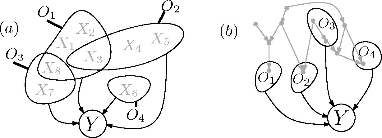
Proposition 1 (Decomposition of information about sets of independent elements). Let$\mathcal{X}=\left\{X_1,\dots ,X_r\right\}$ be mutually independent objects, that is I(X_j : X_[r]nj) = 0 for all j. Let O_[n] = {O₁,…, O_n}, where each$O_i\subseteq \mathcal{X}$ is a non-empty subset of$\mathcal{X}$. For every i ∈ [n], let d_i be maximal, such that O_i has non-empty intersection with d_i −1 sets out of O_[n] distinct from O_i. Then, the information about the O_[n] can be bounded from below by:

$$I(Y:O_{[n]})\ge {\displaystyle \sum _{i=1}^n\frac{1}{d_i}I(Y:O_i)}.$$

(7)

For an illustration, see Figure 3a. Even though the proposition is actually a corollary of the following theorem, its proof is given in Appendix B, since it is, unlike the theorem, independent of graph-theoretic notions.

As a trivial example, consider the case where $O_1=O_2=O\subseteq \mathcal{X}$ are identical subsets. Then, d₁ = d₂ = 2 and:

$$I(Y:O)=\frac{1}{2}I(Y:O_1)+\frac{1}{2}I(Y:O_2),$$

hence equality holds in (7). In general, if there is an element in O_i that is also in k −1 different sets O_j, then d_i ≥k, and we account for this redundancy in dividing the single information I(Y : O_i) by at least k.

Independent elements can always be modeled as root nodes of a DAG. The following theorem, which is our main result, generalizes the proposition by connecting the information about observations O_i to the intersection structure of associated ancestral sets. For a given DAG G, a set of nodes A is called ancestral, if for every edge v → w in G, such that w is in A, also v is in A. Further, for a subset of nodes S, we denote by an(S) the smallest ancestral set that contains S. Elements of an(S) will be called ancestors of S.

Theorem 1 (Decomposition of ancestral information). Let G be a DAG model of an observation of elements O_[n] = {O₁,…, O_n}. For every i, let d_i be the maximal number, such that the intersection of an(O_i) with d_i −1 distinct sets an$\left(O_i{}_{{}_1}\right),\dots ,an\left(O_{i_{d-1}}\right)$ is non-empty. Then, the information about all ancestors of O_[n] can be bounded from below by:

$$I(Y:an(O_{[n]})\ge {\displaystyle \sum _{i=1}^n\frac{1}{d_i}I(Y:an(O_i))\ge {\displaystyle \sum _{i=1}^n\frac{1}{d_i}I(Y:O_i}}).$$

(8)

Furthermore, if Y only depends on whole system$\mathcal{X}$ through the O_[n], that is:

$$Y╨\mathcal{X}\backslash (O_{[n]}\cup \{Y\})|O_{[n]}$$

(9)

we obtain an inequality containing only known values of mutual information:

$$I(Y:O_{[n]})\ge {\displaystyle \sum _{i=1}^n\frac{1}{d_i}I(Y:O_i)}.$$

(10)

The proof is given in Appendix C, and an example is illustrated in Figure 3b. If all quantities except the structural parameters d_i are known, the inequality (10) can be used to obtain information about the intersection structure among the O_i that is encoded in the d_i, provided that the independence assumption (9) holds. Even if (9) does not hold, but information on an upper bound of I(Y : an(O_[n])) is available (e.g., in terms of the entropy of Y), information about the intersection structure may be obtained from (8). The following corollary additionally provides a bound on the minimum information about ancestral sets.

Corollary 1 (Inference of common ancestors, local version). Given an observation of elements O_[n] ={O₁,…, O_n}, assume that for natural numbers c = (c₁,…, c_n) with (1 ≤ c_i ≤n −1), we observe:

$${ϵ}_{\mathbf{c}}:={\displaystyle \sum _{i=1}^n\frac{1}{c_i}I(Y:O_i)}-I(Y:an(O_{[n]}))>0.$$

(11)

Let G be an arbitrary DAG model of the observation. For every O_i, let$A_{c_i}{}_{+1}$ be the set of common ancestors in G of O_i and at least c_i elements of O_[n] different from O_i. Then, the joint information about all common ancestors can be bounded from below by:

$$I(Y:{\displaystyle {\cup }_{i=1}^n{A}_{c_i}+1})\ge {\left({\displaystyle \sum _{i=1}^n\frac{1}{c_i}-1}\right)}^{-1}{ϵ}_{\mathbf{c}}>0.$$

In particular, {or at least one index i ∊ [n], we must have$A_c{}_{{}_i}+1\ne \varnothing$; hence, there exists a common ancestor of O_i and at least c_i elements of O_[n] different from O_i.

The proof is given in Appendix D. Theorem 1 and its corollary are our most general results, but due to the ease of interpretation, we illustrate them in the next section only in the special case in which all c_i are equal (Corollary 2) to obtain a lower bound on the information about all common ancestors of at least c + 1 elements O_i.

To conclude this section, we ask what is the maximum amount of information that one can expect to obtain about the intersection structure of ancestral sets of a DAG model of observations. The main requirement for a DAG model G is that it fulfills the local Markov condition with respect to some larger set X of elements. This will remain true if we add nodes and arbitrary edges in a way that G remains acyclic. Therefore, if G contains a common ancestor of c elements, we can always construct a DAG model G′ that contains a common ancestor of more than c elements (e.g., the DAG model on the right-hand side of Figure 1 can be transformed into the one on the left-hand side). We conclude that without adding minimality requirements for the DAG models (such as the causal faithfulness assumption [2]), only assertions on ancestors of a minimal number of nodes can be made.

4. Structural Implications of Redundancy and Synergy

The results of the last section can be related to the notions of redundancy and synergy. In the context of neuronal information processing, it has been proposed to capture the redundancy and synergy of elements O_[n] = {O₁,…, O_n} with respect to another element Y using the function:

$$r(Y):={\displaystyle \sum _{i=1}^{n}I(Y:O_i)-I(Y:O_{[n]})},$$

(12)

where I is a measure of mutual information [13–15]. Thus, r relates information that Y has about the single elements to information about the whole set.

If the sum of information about the single O_i is larger than the information about whole set (r(Y) > 0), the O_[n] are said to be redundant with respect to Y. This may be the case if Y “contains” information that is shared by multiple O_i. In general, if the O_i do not share any information, that is if they are mutually independent, then they can not be redundant with respect to any Y (this follows from Lemma 3).

On the other hand, if the information of Y about the whole set of elements is larger than that about its single elements (r(Y) < 0), the O_[n] are called synergistic with respect to Y. This may, for example, be the case if Y is generated through a function Y = f(O₁,…, O_n) and the function value contains little information about each argument (as is the case for the parity function; see below). If, instead, Y is a copy of the O_[n], then r(Y) ≥ 0, and thus, the O_[n] are not synergistic with respect to Y. To connect our results to the introduced notion of redundancy and synergy, we introduce the following version of r parametrized by a parameter c ∈ {1,…, n}:

$$r_c(Y):=\frac{1}{c}{\displaystyle \sum _{i=1}^{n}I(Y:O_i)}-I(Y:O_{[n]}).$$

(13)

Intuitively, if r_c(Y) > 0 for large c, then the O_i are highly redundant with respect to Y. Corollary 1 of the last section implies that high redundancy implies common ancestors of many O_i.

Corollary 2 (Redundancy explained structurally). Let an observation of elements O_[n] = {O₁,…, O_n} be given by the values of I(Y : O_S) for any subset S ⊆ [n]. If r_c(Y) > 0, then in any DAG model of the observation in which Y only depends on$\mathcal{X}$ through O_[n] [16], there exists a common ancestor of at least c + 1 elements of O_[n].

In the following two subsections, we discuss this result in more detail for the cases in which the observed elements are discrete random variables and binary strings.

4.1. Common Ancestors of Discrete Random Variables

Let X_[n] = {X₁,…, X_n} and Y be discrete random variables with joint distribution p(X_[n]; Y), and let I denote the usual measure of mutual information given by the Kullback–Leibler divergence of p from its factorized distribution [7]. If Y = X_[n] is a copy of the X_[n], then I(Y : X_[n]) = H(X_[n]), where H denotes the Shannon entropy. In this case, the redundancy r₁(X_[n]) is equal to the multi-information [17] of the X_[n]. Moreover, r_c gives rise to a parametrized version of multi-information:

$$I_c(X_1,\dots ,X_n):={\displaystyle \sum _{i-1}^n\frac{1}{c}H(X_i)-H(X_{[n]}),}$$

(14)

and from Corollary 1, we obtain

Theorem 2 (Lower bound on entropy o{ common ancestors). Let X_[n] be jointly-distributed discrete random variables. If I_c(X_[n]) > 0, then in any Bayesian net containing the X_[n], there exists a common ancestor of strictly more than c variables out of the X_[n]. Moreover, the entropy of the set A_c+1 of all common ancestors of more than c variables is lower bounded by:

$$H(A_{c+1})\ge \frac{c}{n-c}{I}_c(X_{[n]}).$$

(15)

We continue with a few remarks to illustrate the theorem:

• Setting c = 1, the theorem states that, up to a factor 1=(n 1), the multi-information I₁ is a lower bound on the entropy of common ancestors of more than two variables. In particular, if I₁(X_[n]) > 0, any Bayesian net containing the X_[n] must have at least an edge.
• Conversely, the entropy of common ancestors of all of the elements X₁,…, X_n is lower bounded by (n −1)I_n−1(X_[n]). This bound is not trivial whenever I_n−1(X_[n]) > 0, which is, for example, the case if the X_i are only slightly disturbed copies of some not necessarily observed random variable (see the example below).
• We emphasize that the inferred common ancestors can be among the elements X_i themselves. Unobserved common ancestors can only be inferred by postulating assumptions on the causal influences among the X_i. If, for example, all of the X_i were measured simultaneously, a direct causal influence among the X_i can be excluded, and any dependence or redundancy has to be attributed to unobserved common ancestors.
• Finally, note that I_c > 0 is only a sufficient, but not a necessary condition for the existence of common ancestors. However, we know that the information-theoretic information provided by I_c is used in the theorem in an optimal way. By this, we mean that we can construct distributions p(X_[n]), such that I_c(X_[n]) = 0 for a given c, and no common ancestors of c+1 nodes have to exist.

We conclude this section with examples:

Example 1 (Three variables). Let X₁; X₂ and X₃ be three binary variables. Then I₂(X₁; X₂; X₃) > 0 if and only if

$$H\left(X_1\right)+H\left(X_2\right)+H\left(X_3\right)>2H\left(X_1,X_2,X_3\right).$$

In this case, there must exist a common ancestor of all three variables in any Bayesian net that contains them. In particular, any Bayesian net corresponding to the DAG on the right-hand side of Figure 1 can be excluded as a model.

Example 2 (Synchrony and interaction among random variables). Let X₁ = X₂ = ⋯= X_n be identical random variables with non-vanishing entropy h. Then, in particular, I_n−1(X_[n]) = (n−1)⁻¹h > 0, and we can conclude that there has to exist a common ancestor of all n nodes in any Bayesian net that contains them.

Example 3 (Interaction of maximal order). In contrast to the synchronized case, let X₁; X₂,…, X_n be binary random variables taking values in {−1,1}, and assume that the joint distribution is of pure n-interaction [18], that is for some β ≠ 0, it has the form

$$p_{\beta }(x_1,\dots ,x_n):=\frac{1}{Z_{\beta }}\exp (\beta x_1{x}_2\cdots x_n),$$

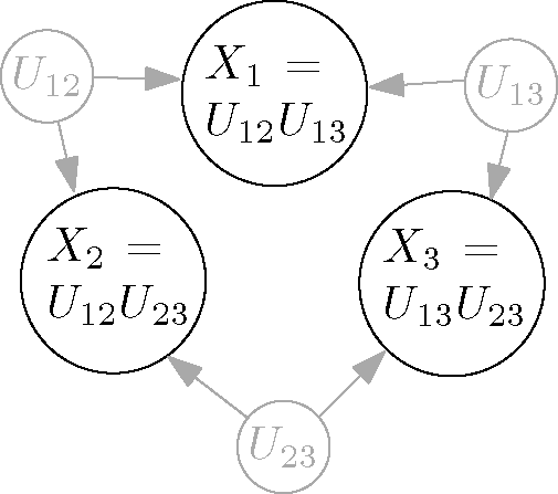
where Z is a normalization constant. It can be shown that there exists a Bayesian net including the X_[n], in which common ancestors of at most two variables exist. This is illustrated in Figure 4 for three variables and in the limiting case β = ∞ in which each X_i is uniformly distributed and X₁ =X₂·X₃. We found it somewhat surprising that, contrary to synchronization, higher order interaction among observations does not require common ancestors of many variables.

4.2. Common Ancestors in String Manipulation Processes

In some situations, it is not convenient or straightforward to summarize an observation in terms of a joint probability distribution of random variables. Consider for example cases in which the data comes from repeated observations under varying conditions (e.g., time series). A related situation is given if the number of samples is low. Janzing and Schölkopf [4] argue that causal inference in these situations still should be possible, provided that the observations are sufficiently complex. To this end, they developed a framework for causal inference from single observations that we describe now briefly. Assume we have observed two objects A and B in nature (e.g., two carpets), and we encoded these observations into binary strings a and b. If the descriptions of the observations in terms of the strings a and b are sufficiently complex and sufficiently similar (e.g., the same pattern on the carpets), one would expect an explanation of this similarity in terms of a mechanism that relates these two strings in nature (are the carpets produced by the same company?). It is necessary that the descriptions are sufficiently complex, as an example of [4] illustrates: assume the two observed strings are equal to the first hundred digits of the binary expansion of π; hence, they can be generated independently by a simple rule. If this is the case, the similarity of the two strings would not be considered as strong evidence for the existence of a causal link. To exclude such cases, the Kolmogorov complexity [19] K(s) of a string s has been used as the measure of complexity. It is defined as the length of the shortest program that prints out s on a universal (prefix-free) Turing machine. With this definition, strings that can be generated using a simple rule, such as the constant string s = 0⋯0 or the first n digits of the binary expansion of π, are considered simple, whereas it can be shown that a random string of length n is complex with high probability. Kolmogorov complexity can be transformed into a function on sets of strings by choosing a suitable concatenation function ⟨, ⟩, such that K(s₁,…, s_n) = K(⟨s₁, ⟨s₂,…, ⟨s_n−1, s_n⟩ …⟩).

The algorithmic mutual information [8] of two strings a and b is then equal to the sum of the lengths of the shortest programs that generate each string separately minus the length of the shortest program that generates the strings a and b:

$$I\left(a:b\right)\stackrel{+}{=}K(a)+K(b)-K(a,b),$$

where ⩲ stands for equality up to an additive constant that depends on the choice of the universal Turing machine. Analogous to Reichenbach’s principle of common cause, [4] postulates a causal relation among a and b whenever I(a : b) is large, which is the case if the complexities of the strings are large and both strings together can be generated by a much shorter program than the programs that describe them separately.

In formal analogy to the probabilistic case, algorithmic mutual information can be extended to a conditional version defined for sets of strings A, B, C ⊆ {s₁,…, s_n} as:

$$I\left(A:B|C\right)\stackrel{+}{=}K\left(A\cup C\right)+K\left(B\cup C\right)-K(A\cup B\cup C)-K\left(C\right).$$

Intuitively, I(A : B |C) is the mutual information between the strings of A and the strings of B if the shortest program that prints the strings in C has been provided as an additional input. Based on this notion of conditional mutual information, the causal Markov condition can be formulated in the algorithmic setting. It can be proven [4] to hold for a directed acyclic graph G on strings s₁,…, s_n if every s_i can be computed by a simple program on a universal Turing machine from its parents and an additional string n_i, such that the n_i are mutually independent. Without going into the details, we sum up by stating that DAGs on strings can be given a causal interpretation, and it is therefore interesting to infer properties of the class of possible DAGs that represent the algorithmic conditional independence relations.

In the algorithmic setting, our result can be stated as follows:

Theorem 3 (Inference of common ancestors of strings). Let O_[n] = {s₁,…, s_n} be a set of binary strings. If for a number c, (1≤ c ≤ n −1):

$$\frac{1}{c}{\displaystyle \sum _{i=1}^{n}K(s_i)}-K(s_1,\dots ,s_n)\stackrel{+}{\ge }0,$$

then there must exist a common ancestor of at least c+1 strings out of O_[n] in any DAG model of the O_[n]. (Here, $\stackrel{+}{\ge }$ means up to an additive constant dependent only on the choice of a universal Turing machine, on c and on n.)

Proof. As described, algorithmic mutual information is an information measure in our sense only up to an additive constant depending on the choice of the universal Turing machine. However, one can check that in this case, the decomposition of mutual information (Theorem 1) holds up to an additive constant that depends additionally on the number of strings n and the chosen parameter c. The result on Kolmogorov complexities follows by choosing Y = (s₁,…, s_n), since $K(s_i)\stackrel{+}{=}I\left(Y:s_i\right)$.

Thus, highly-redundant strings require a common ancestor in any DAG model. Since the Kolmogorov complexity of a string s is uncomputable, we have argued in recent work [5] that it can be substituted by a measure of complexity in terms of the length of a compressed version of s with respect to a chosen compression scheme (instead of a universal Turing machine), and the above result should still hold approximately.

4.3. Structural Implications from Synergy?

We saw that large redundancy implies common ancestors of many elements, and we may wonder whether structural information can be obtained from synergy in a similar way. This seems not to be possible, since synergy is related to more fine-grained information (information about the mechanisms), as the following example shows: Assume the observations O_[n] are mutually independent. Then, any DAG is a valid DAG model, since the local Markov condition will always be satisfied. We also now that r(Y)≤ 0, but it turns out that the amount of synergy crucially depends on the way that Y has processed the information of the O_[n] (and therefore, not on a structural property among the O_[n] themselves). To see this, let the observations O_i be binary random variables, which are mutual independent and distributed uniformly, such that:

$$\begin{array}{cc}p(O_{[n]})={\displaystyle \prod _{i=1}^{n}p(O_i)}& \text{and}p(O_i=1)=p(O_i=0)=1/2\end{array}.$$

Further, let Y = (O_i ⊕O_j)_i<j be a function of the observations (addition is modulo two). Then, the O_[n] are highly synergistic with respect to Y, that is r₁(Y) = −(n−1) log 2. On the other hand, if Y = O₁ ⊕⋯⊕O_n, then r₁(Y) = −log 2 only.

Nevertheless, it is an easy observation that synergy with respect to Y can be related to an increase of redundancy after conditioning on Y. Since I(·|Y) is a measure of mutual information, as well, we define a conditioned version of r in a canonical way as:

$$r_c(Z|Y)=\frac{1}{c}{\displaystyle \sum _{i=1}^{n}I(Z:O_i|Y)}-I(Z:O_{[n]}|Y),$$

with respect to some observation Z. If I can be evaluated on non-disjoint subsets, that is if we can choose Z = O_[n], we have the following:

Proposition 2 (Synergy from increased redundancy induced by conditioning). Let O_[n] = {O₁,…, O_n} and Y be arbitrary elements on which a mutual information function I is defined. Then:

$$r_c(Y)=r_c\left(O_{[n]}\right)-r_c(O_{[n]}|Y),$$

hence if conditioning on Y increases the redundancy of O_[n] with respect to itself, then r_c(Y) < 0 and the O_[n] are synergistic with respect to Y.

Proof. Using the chain rule, we derive

$$r_c\left(O_{[n]}\right)-r_c(O_{[n]}|Y)=r_c(Y)-r_c\left(Y|O_{[n]}\right)=r_c(Y),$$

where the last equality follows because r_c(Y|O_[n]) = 0.

Continuing the example of binary random variables above, mutual independence of the O_[n] is equivalent to r₁(O_[n]) = 0 and, therefore, using the proposition r₁(Y) =−r₁(O_[n]|Y). Thus, if Y = O₁⊕⋯ ⊕O_[n],

$$r_1(Y)=-r_1(O_{[n]}|Y)=H(O_{[n]}|Y)-{\displaystyle \sum _{i=1}^{n}H(O_i|Y)=-\log 2},$$

as already noted above.

5. Conclusions

Based on a generalized notion of mutual information, we proved an inequality describing the decomposition of information about a whole set into the sum of information about its parts. The decomposition depended on a structural property, namely the existence of common ancestors in a DAG. We connected the result to the notions of redundancy and synergy and concluded that large redundancy implies the existence of common ancestors in any DAG model. Specialized to the case of discrete random variables, this means that large stochastic dependence in terms of multi-information needs to be explained through a common ancestor (in a Bayesian net) acting as a broadcaster of information.

Much work has been done already that examined the restrictions that are imposed on observations by graphical models that include latent variables. Pearl [1,20] already investigated constraints imposed by the special instrumental variable model. Furthermore, Darroch et al. [21] and, recently, Sullivant et al. [22] looked at linear Gaussian graphical models and determined constraints in terms of the entries on the covariance matrix describing the data (tetrad constraints). Further, methods of algebraic statistics were applied (e.g., [23]) to derive constraints that are induced by latent variable models directly on the level of probabilities. In general, this does not seem to be an easy task due to the large number of variables involved. Information theory, on the other hand, provides efficient methods for comparatively easy derivations of “macroscopic” constraints, the main subject of the present article (see also [24]).

Since the initial publication of this manuscript as a preprint [25], subsequent progress has been made on the problem of inferring DAG models from partial observations. In [26], the problem is treated in the wider context of inferring possible joint distributions from restrictions on marginals. There, an algorithm is presented that, even though computationally demanding, computes all Shannon-type entropic inequalities for given marginal constraints. Furthermore, it has turned out that entropic inequalities are useful in quantum physics where they restrict possible theories of data generation in more general settings than the ones using Bell inequalities (see, e.g., [27–30]). Moreover, we would like to mention that meanwhile, information measures for causal inference among strings based on compression length have been proposed [31], thus extending the possible applications of inequalities like the ones presented in this article.

Initiated by the work [32] of Williams and Beer, recent progress has been made related to the concepts of synergy and redundancy [33–35]. These works, however, do not address any causal interpretations. We think that the general methodology of connecting the redundancy and synergy of observations to properties of the class of possible DAG models will add new insights to this research direction.

Our generalized notion r_c of redundancy (see (13)) has been used by Ver Steeg and Galstyan as an objective function for hierarchical representations of high-dimensional data [36,37], where the optimization is taken with respect to the variable Y.

Finally, we would like to mention the works [38] and [39] of one of us, which were based on our present article. In the article [38], our lower bound on the entropy of common ancestors, the inequality (15), is interpreted as a special linear inequality of entropic terms. The solution sets of such information inequalities are studied as the basis for casual inference. The work [39] gives a tight upper bound on our parametrized version I_c(X₁,…, X_n) of multi-information (see (14)) and derives a method for discriminating between causal structures in Bayesian networks given partial observations.

References and Notes

- Pearl, J. Causality; Cambridge University Press: Cambridge, UK, 2000. [Google Scholar]
- Spirtes, P.; Glymour, C.; Scheines, R. Causation, Prediction, and Search, 2nd ed.; Adaptive Computation and Machine Learning series; The MIT Press: Cambridge, MA, USA, 2001. [Google Scholar]
- Lauritzen, S.L. Graphical Models; Oxford Statistical Science Series; Oxford University Press: Oxford, UK, 1996. [Google Scholar]
- Janzing, D.; Schölkopf, B. Causal inference using the algorithmic Markov condition. IEEE Trans. Inf. Theory. 2010, 56, 5168–5194. [Google Scholar]
- Steudel, B.; Janzing, D.; Schölkopf, B. Causal markov condition for submodular information measures, Proceedings of the 23rd Annual Conference on Learning Theory, Haifa, Israel, 17–19 June 2010; pp. 464–476.
- Reichenbach, H. The Direction of Time; University of Califonia Press: Oakland, CA, USA, 1956. [Google Scholar]
- Cover, T.M.; Thomas, J.A. Elements of Information Theory, 2nd ed.; Wiley: New York, NY, USA, 2006. [Google Scholar]
- Gács, P.; Tromp, J.T.; Vitányi, P.M. Algorithmic statistics. IEEE Trans. Inf. Theory. 2001, 47, 2443–2463. [Google Scholar]
- Pearl, J. Probabilistic Reasoning in Intelligent Systems: Networks of Plausible Inference; Morgan Kaufmann Publishers Inc: San Francisco, CA, USA, 1988. [Google Scholar]
- Mutual information of composed quantum systems satisfies the definition as well, because it can be defined in formal analogy to classical information theory if Shannon entropy is replaced by von Neumann entropy of a quantum state. The properties of mutual information stated above have been used to single out quantum physics from a whole class of no-signaling theories [42].
- Dawid, A.P. Conditional independence in statistical theory. J. R. Stat. Soc. Ser. B (Methodol.). 1979, 41, 1–31. [Google Scholar]
- Madiman, M.; Tetali, P. Information inequalities for joint distributions, with interpretations and applications. IEEE Trans. Inf. Theory. 2010, 56, 2699–2713. [Google Scholar]
- Schneidman, E.; Bialek, W.; Berry, M.J., II. Synergy, redundancy, and independence in population codes. J. Neurosci. 2003, 23, 11539–11553. [Google Scholar]
- Latham, P.E.; Nirenberg, S. Synergy, redundancy, and independence in population codes, revisited. J. Neurosci. 2005, 25, 5195–5206. [Google Scholar]
- Schneidman, E.; Still, S.; Berry, M.J., II; Bialek, W. Network information and connected correlations. Phys. Rev. Lett. 2003, 91, 238701. [Google Scholar]
- We formulate the independence assumption as , where denotes all nodes of the DAG-model different from the nodes in O[n] and Y. Note that this assumption does not hold in the original context in which r has been introduced. There, Y is the observation of a stimulus that is presented to some neuronal system and the Oi represent the responses of (areas of) neurons to this stimulus.
- Studeny, M.; Vejnarová, J. The multiinformation function as a tool for measuring stochastic dependence. In Learning in Graphical Models; Jordan, M.I., Ed.; Kluwer Academic Publishers: Norwell, MA, USA, 1998; pp. 261–297. [Google Scholar]
- This terminology is motivated by the general framework of interaction spaces proposed and investigated by Darroch et al. [21] and used by Amari [43] within information geometry.
- Li, M.; Vitányi, P. An Introduction to Kolmogorov Complexity and Its Applications (Text and Monographs in Computer Science); Springer: Berlin, Germany, 2007. [Google Scholar]
- Pearl, J. On the testability of causal models with latent and instrumental variables, Proceedings of the 11th Conference on Uncertainty in Artificial Intelligence (UAI), Montreal, QU, USA, 18–20 August 1995; pp. 435–443.
- Darroch, J.N.; Lauritzen, S.L.; Speed, T.P. Markov fields and log-linear interaction models for contingency tables. Ann. Stat. 1980, 8, 522–539. [Google Scholar]
- Sullivant, S.; Talaska, K.; Draisma, J. Trek separation for gaussian graphical models. Ann. Stat. 2010, 38, 1665–1685. [Google Scholar]
- Riccomagno, E.; Smith, J.Q. Algebraic causality: Bayes nets and beyond 2007, arXiv, 0709.3377.
- Ay, N. A refinement of the common cause principle. Discret. Appl. Math. 2009, 157, 2439–2457. [Google Scholar]
- Steudel, B.; Ay, N. Information-Theoretic Inference of Common Ancestors 2010, arXiv, 1010.5720.
- Fritz, T.; Chaves, R. Entropic inequalities and marginal problems. IEEE Trans. Inf. Theory. 2013, 59, 803–817. [Google Scholar]
- Chaves, R.; Luft, L.; Gross, D. Causal structures from entropic information: geometry and novel scenarios. New J. Phys. 2014, 16, 043001. [Google Scholar]
- Fritz, T. Beyond Bell’s theorem: correlation scenarios. New J. Phys. 2012, 14, 103001. [Google Scholar]
- Chaves, R.; Majenz, C.; Gross, D. Information-theoretic implications of quantum causal structures. Nat. Commun. 2015, 6. [Google Scholar] [CrossRef]
- Henson, J.; Lal, R.; Pusey, M.F. Theory-independent limits on correlations from generalized Bayesian networks. New J. Phys. 2014, 16, 113043. [Google Scholar]
- Steudel, B.; Janzing, D.; Schölkopf, B. Causal Markov condition for submodular information measures, Proceedings of the 23rd Annual Conference on Learning Theory, Haifa, Israel, 17–19 June 2010; Kalai, A.T., Mohri, M., Eds.; OmniPress: Madison, WI, USA; pp. 464–476.
- Williams, P.; Beer, R. Nonnegative decomposition of multivariate information 2010, arXiv, 1004.2515.
- Bertschinger, N.; Rauh, J.; Olbrich, E.; Jost, J.; Ay, N. Quantifying unique information. Entropy 2014, 16, 2161–2183. [Google Scholar]
- Harder, M.; Salge, C.; Polani, D. Bivariate measure of redundant information. Phys. Rev. E 2013, 87, 012130. [Google Scholar]
- Griffith, V.; Koch, C. Quantifying synergistic mutual information 2013, arXiv, 1205.4265.
- Ver Steeg, G.; Galstyan, A. Discovering structure in high-dimensional data through correlation explanation, Prodeedings of Advances in Neural Information Processing System 27, Montréal, QC, Canada, 8–13 December 2014; pp. 577–585.
- Ver Steeg, G.; Galstyan, A. Maximally Informative Hierarchical Representations of High-Dimensional Data, Proceedings of the 18th International Conference on Artificial Intelligence and Statistics (AISTATS), San Diego, CA, USA; 2015.
- Ay, N.; Wenzel, W. On Solution Sets of Information Inequalities. Kybernetika 2012, 48, 845–864. [Google Scholar]
- Moritz, P.; Reichardt, J.; Ay, N. Discriminating between causal structures in Bayesian Networks via partial observations. Kybernetika 2014, 50, 284–295. [Google Scholar]
- In general there may hold additional conditional independence relations among the observations that are not implied by the local Markov condition together with the semi-graphoid axioms. In fact, it is well known that there so called non-graphical probability distributions whose conditional independence structure can not be completely represented by any DAG.
- Verma, T.; Pearl, J. Causal networks: Semantics and expressiveness. Uncertain. Artif. Intell. 1990, 4, 69–76. [Google Scholar]
- Pawłowski, M.; Paterek, T.; Kaszlikowski, D.; Scarani, V.; Winter, A.; Żukowski, M. Information causality as a physical principle. Nature 2009, 461, 1101–1104. [Google Scholar]
- Amari, S.I. Information geometry on hierarchy of probability distributions. IEEE Trans. Inf. Theory. 2001, 47, 1701–1711. [Google Scholar]
Figure 1.
Two causal hypothesis for which the causal Markov condition does not imply conditional independencies among the observations X1, X2 and X3. Thus, they cannot be distinguished using qualitative criteria, like the common cause principle (unobserved variables are indicated as dots). However, the model on the right can be excluded if the dependence among the Xi exceeds a certain bound.
Figure 2.
The graph in (a) shows a directed acyclic graph (DAG) on nodes X1,…, X5 whose observation is modeled by a leaf node Y (e.g., a noisy measurement). (b) A DAG model of observed elements O1 = {X1} and O2 = {X4, X5}.
Figure 3.
(a) Four subsets O1,…, O4 of independent elements X1,…, X8 “observed by” Y. Note that the intersection of three sets Oi is empty; hence, di ≤ 2 for all i = 1,…, 4 in Proposition 1 and, therefore,
. (b) A DAG model in gray. The observed elements O1,…, O4 are subsets of its nodes. One can check that the DAG does not imply any conditional independencies among the Oi (e.g., with the help of the d-separation criterion; see Appendix A). Nevertheless, there is no common ancestor of all four observations
. Since Y only depends on the Oi, the inequality (10) of Theorem 1 implies
.
Figure 4.
The figure illustrates that higher order interaction among observed random variables can be explained by a Bayesian net in which only common ancestors of two variables exist. More precisely, all random variables are assumed to be binary with values in {−1, 1}, and the unobserved common ancestors Uij are mutually independent and uniformly distributed. Further, the value of each observation Xi is obtained bythe product of the values of its two ancestors. Then, the resulting marginal distribution p(X1, X2, X3) is of higher order interaction: it is related to the parity function p(X1 = x1, X2 = x2, X3 = x3) =
if x1x2x3 = 1, and zero otherwise.
© 2015 by the authors; licensee MDPI, Basel, Switzerland This article is an open access article distributed under the terms and conditions of the Creative Commons Attribution license (http://creativecommons.org/licenses/by/4.0/).
Share and Cite
MDPI and ACS Style
Steudel, B.; Ay, N. Information-Theoretic Inference of Common Ancestors. Entropy 2015, 17, 2304-2327. https://0-doi-org.brum.beds.ac.uk/10.3390/e17042304
AMA Style
Steudel B, Ay N. Information-Theoretic Inference of Common Ancestors. Entropy. 2015; 17(4):2304-2327. https://0-doi-org.brum.beds.ac.uk/10.3390/e17042304
Chicago/Turabian StyleSteudel, Bastian, and Nihat Ay. 2015. "Information-Theoretic Inference of Common Ancestors" Entropy 17, no. 4: 2304-2327. https://0-doi-org.brum.beds.ac.uk/10.3390/e17042304