Identifying the Most Relevant Lag with Runs

Abstract

In this paper, we propose a nonparametric statistical tool to identify the most relevant lag in the model description of a time series. It is also shown that it can be used for model identification. The statistic is based on the number of runs, when the time series is symbolized depending on the empirical quantiles of the time series. With a Monte Carlo simulation, we show the size and power performance of our new test statistic under linear and nonlinear data generating processes. From the theoretical point of view, it is the first time that symbolic analysis and runs are proposed to identifying characteristic lags and also to help in the identification of univariate time series models. From a more applied point of view, the results show the power and competitiveness of the proposed tool with respect to other techniques without presuming or specifying a model.

1. Introduction

In this paper, we are particularly interested in providing new statistical tools that help in the process of modelling univariate time series processes. We are focused on the selection of the appropriate time lags when data faced by the modeller might potentially come from either a linear or a nonlinear dynamic time process. Needless to say, a correct estimate of the lag is essential in forecasting basically because the introduction of delayed information into the dynamic models significantly changes their asymptotic properties. Traditionally, autocorrelation and partial autocorrelation coefficients have been utilized by empirical modellers in specifying the appropriate delays. However, it is well established [1] that processes with zero autocorrelation could still exhibit high order dependence or nonlinear time dependence. This is the case for some bilinear processes and even for purely deterministic chaotic models, among others. In general, autocorrelation-based procedures may be misleading for nonlinear models, and so might fail to detect important nonlinear relationships present in the data, and are therefore of limited utility in detecting appropriate time delays (lags), especially in those scenarios where nonlinear phenomena are more the rule than the exception. The relevance of non-linear time dependent processes in science and social sciences, as well as in macroeconomics and finance, is well established. However, statistical tools that help to specify what lag(s) to use in a nonlinear description of an observed time series are scarce.

From a statistical point of view, this situation has motivated the development of tests for serial independence (see [2] for a review) with statistical power against alternative hypotheses that exhibit general types of dependence. The vast majority of these statistical tests are of nonparametric nature, hence trying to avoid restrictive assumptions on the marginal distributions of the model. However these tests are not designed for selecting relevant lags. This partly explains the relative scarcity of nonparametric techniques for investigating lag dependence, regardless the linear or nonlinear nature of the process, which is an aspect that is unknown in most of the practical cases. Some notable exceptions to this relative scarcity are [3–6]. A common characteristic of most of these techniques is the use of entropy-based measures to identify the correct lag. Particularly, in [5,6], the use of permutation entropy, evaluated at several delay times, is theoretically motived and then applied to identify from a time series the characteristic lag of the generating system. Interesting physical applications of this approach are [7,8]. In order to complete the paper, the new proposal technique is compared with the widely applied autocorrelation function and with recent techniques based on permutation entropy.

In this paper, we construct a new nonparametric runs statistic, based on symbolic analysis, which estimates the lag that best describes a time series sample. The versatile nature of runs tests is well-known for the relevant statistical literature as it has been used for analyzing independence, symmetries, randomness, etc. Furthermore, symbolic analysis is a field of increasing interest in several scientific disciplines (see [9]). It has foundations in information theory and in theory of dynamic systems. For example, properties of symbolic encodings are central to the theory of communication [10]. Furthermore, there is a well-established mathematical discipline, namely, symbolic dynamics, that studies the behavior of dynamical systems. This discipline started in 1898 with the pioneering works of Hadamard, which developed a symbolic description of sequences of geodesic flows, and was later extended by [11], who coined the name of symbolic dynamics. [12] showed that a complete description of the behavior of a dynamical system can be captured in terms of symbols. This observation is crucial for understanding this paper because important characteristics of a random variable can be also captured by analyzing the symbols derived from it.

The paper finally shows that the new approach can be useful for model identification, and it is applied to the a real time series, particularly, to the New York Stock Exchange.

2. Definitions and Notation

Let {X_i}_i∈I be a time series. Assume first that {X_i}_i∈I is a sequence of categorical data with q categories. Denote by n_k the number of elements of the k category. Therefore

$${\displaystyle \sum _{k=1}^q{n}_k=n},$$

where n = |I| is the cardinality of the set of time indexes I. Under this setting we will define a run as a sequence of categories of the same type.

In the case of quantitative (continuous or discrete) data we will encode the sequence {X_i}_i∈I in q different categories for q a positive integer in the following manner. Denote by Q_k the quantile $\frac{kn}{q}$ of {X_i}_i∈I for k = 1, 2…, q − 1. Now we are going to encoded the sequence {X_i}_i∈I as the sequence {X_i}_i∈I where

$$Z_i=\{\begin{array}{ll}1& \mathrm{if}\min \left\{X_i\right\}<X_i\le Q_1\\ k& \mathrm{if}{Q}_{k-1}<X_i\le Q_k\\ q& \mathrm{if}{Q}_k<X_i\le \max \left\{X_i\right\}\end{array}$$

(1)

A run is obtained by encoding the time series {X_i}_i∈I with a finite set of symbols Γ. Then a sequence of symbols of the same type is called a run. In the previous encoding the set of symbols is Γ = {1, 2,…, q} for the symbolization given in Equation (1).

3. Constructing the Statistic

The classical runs test is defined for q = 2 where only two categories or symbols are used. This can be considered in a multinomial scenario with q > 2. For completeness we will give the construction of the runs test for i.i.d (identically and independently distributed) in the multinomial case that was developed in [13].

Let $\mathcal{MR}$ be the random variable counting the number of runs in {X_i}_i∈I (if this sequence is not categorical we will use the symbolization procedure given by Equation (1)). Define the following indicator function

$${\mathcal{I}}_j=\{\begin{array}{ll}1& \mathrm{if}{X}_{j-1}\ne X_j\\ 0& \text{otherwise}.\end{array}$$

(2)

The variable ${\mathcal{I}}_j$ is a Bernoulli variable B(p) with probability of success

$$p=\frac{{\displaystyle \sum _{i=1}^q{n}_i(n-n_i)}}{n(n-1)}$$

(3)

for all j = 2, 3,…, n. Then the statistic ${\mathcal{MR}}_q$ remains as:

$${\mathcal{MR}}_q=1+{\displaystyle \sum _{j=2}^n{\mathcal{I}}_j}$$

(4)

and its expected value is

$$E({\mathcal{MR}}_q)=1\frac{{\displaystyle \sum _{i=1}^q{n}_i(n-n_i)}}{n}.$$

(5)

The estimation of the variance of ${\mathcal{MR}}_q$ is more complicated and can be computed as follows (see [13] for a detailed explanation of the computation):

$$\begin{array}{l}{\sigma }_{{\mathcal{MR}}_q}^2=(n-1)p(1-(n-1)p)+\frac{2{\displaystyle \sum _{i\ne j}{n}_i{n}_j(2n-n_i-n_j-2)}}{n(n-1)}+\\ \frac{{\displaystyle \sum _{i\ne j}{n}_i{n}_j((n_i-1)(n-n_i-1)+(n_j-1)(n-n_j-1)+}{\displaystyle \sum _{k\ne i,j}{n}_k(n-n_k-2))}}{n(n-1)}\end{array}$$

(6)

When the lag order of the underlying process is known, say p, one can consider the following p time series

$$\begin{array}{c}{\mathrm{\Gamma }}_1=\{X_1,X_{1+p},X_{1+2p},\dots ,X_{1+tp},\dots \}\\ {\mathrm{\Gamma }}_2=\{X_2,X_{2+p},X_{2+2p},\dots ,X_{2+tp},\dots \}\\ ⋮\\ {\mathrm{\Gamma }}_p=\{X_p,X_{p+p},X_{p+2p},\dots ,X_{p+tp},\dots \}\end{array}$$

For each one of the time series Γ_j one can compute the normalized statistic

$${\mathrm{\Upsilon }}_q^j=\frac{{\mathcal{MR}}_q-E({\mathcal{MR}}_q)}{{\sigma }_{{\mathcal{MR}}_q}}.$$

Under the null of i.i.d. the statistic ${\mathrm{\Upsilon }}_q^j$ is asymptotically normal distributed (see [13]).

Notice that if p is the most relevant lag in the underlying data generating process, then the runs statistic $\mathcal{MR}$ measured on each Γ_j will differ from its expected value more than for any other lag. Then we define

$${\mathrm{\Lambda }}_q^p=\left|\frac{{\displaystyle \sum _{j=1}^p{\mathrm{\Upsilon }}_q^j}}{\sqrt{p}}\right|$$

as the absolute value of the sum of the statistic ${\mathrm{\Upsilon }}_q^j$ for j = 1, 2,…, p divided by the square root of p. In the case that the time series {X_i}_i∈I is i.i.d., and therefore no relevant lags are present, the distribution of the statistic ${\mathrm{\Lambda }}_q^p$ is the folded standard normal distribution, and hence its expected value is $E({\mathrm{\Lambda }}_q^p)=\sqrt{\frac{2}{\pi }}\approx 0.7979$.

Hence, if p₀ is the most relevant lag describing the dynamics of the underlying data generating process then

$${\mathrm{\Lambda }}_q^{p0}=\max \left\{{\mathrm{\Lambda }}_q^p\right|p\in \mathbb{N}\}$$

and ${\mathrm{\Lambda }}_q^{p0}$ has to be greater than $\sqrt{\frac{2}{\pi }}$.

4. Monte Carlo Simulation Experiments

In order to show the statistical power performance of the ${\mathrm{\Lambda }}_q^{p0}$ statistic under different scenarios, we have considered (and therefore simulated) the following data generating processes (DGPs) because of its rich linear and nonlinear variety. The models are the following:

• DGP 1 X_t = 0.3X_t−1 + ∈_t,
• DGP 2 X_t = |0.5X_t−1|^0.8 + ∈_t,
• $\mathrm{DGP}3X_t=0.8{\in }_{t-2}^2+{\in }_t,$
• DGP 4 X_t = 0.7∈_t−1X_t−2+∈_t,
• $\mathrm{DGP}5X_t=\sqrt{h_t{\in }_t},h_t=1+0.8X_{t-1}^2,$
• DGP 6 X_t = 4X_t−1(1 − X_t−1),
• DGP 7 X_t = ∈_t ∼ N(0, 1).

We have considered mainly nonlinear models, but also some linear ones in order to study and compare the procedure with other statistical tools that are commonly used for model specification. Model 1 is a linear processes while Models 2–6 are nonlinear. DGP 1 is an AR1 autoregressive with decaying memory at lag order 1, so the procedure should detect (select) p = 1. DGP 2 is a nonlinear autoregressive model of order 1. DGP 3 is a nonlinear moving average processes of order 2, and then the statistical process is expected to select p = 2. DGP 4 is bilinear with white noise characteristic of orders 2 and 1. Conditional heteroskedastic models (i.e., those with structure in the conditional variance) are commonly employed in financial applications (for example time series that show periods of high and low market uncertainty), and accordingly, it is interesting to know about the behavior of the procedure under these kind of nonlinearities in the conditional variance, so we have included DGP 5. Finally, a purely deterministic model (DGP 6) and an independent and identically distributed stochastic process (DGP 7) are incorporated as they represent two models of opposite nature.

To evaluate the performance of the nonparametric method in finite samples, we compute 1000 Monte Carlo replications of each model, and we consider 6 lags (p). In general, experiments using large data sets are desirable, however situations do occur in which the number of available data is small. Statistical techniques, especially those that are model-free, as it is the case, are very sensitive to the number of observations. For this reason, in the Monte Carlo experiment, we study the effect of small sample size on the outcome of the statistical procedure. We present the results for several different sample sizes, namely, T = 120, 360, 500, 1000, 5000 and 10,000. In order to estimate ${\mathrm{\Lambda }}_q^p$ it is necessary to fix the number of quantiles that we will use to symbolise the time series under consideration, in this case we select q = 3, thus only 3 symbols are used to obtain a conclusion about the dynamic structure of the time series under study.

As mentioned in the introduction, we also compare the proposed method with the widely applied autocorrelation functions and with the permutation entropy based technique, as used in [5], which is related to [6] in the sense that both papers look for the lag that minimizes the permutation entropy. In order to apply the procedure we also fix the embedding reconstruction dimension at m = 3, and we will refer to it as h₃.

Table 1. Comparison ${\mathrm{\Lambda }}_3^p$ against ACF, PAF and h₃ for DGP 1: X_t = 0.3X_t−1 + ∈_t.

T		p = 1	p = 2	p = 3	p = 4	p = 5	p = 6
120	${\mathrm{\Lambda }}_q^p$	57.2	11	7.6	8.2	8.6	7.4
	ACF	90.7	1.9	1.9	1.8	1.9	1.8
	PAF	91.4	2	1.2	1.9	1.7	1.8
	h3	26.4	14.1	12.8	15.2	15.3	16.2
360	${\mathrm{\Lambda }}_q^p$	93.2	1.7	1.2	1.5	1.3	1.1
	ACF	99.7	0.1	0.1	0.1	0	0
	PAF	99.8	0.1	0.1	0	0	0
	h3	50.5	12.0	8.9	8.9	9.2	10.5
500	${\mathrm{\Lambda }}_q^p$	97.8	0.9	0.5	0.3	0.4	0.1
	ACF	100	0	0	0	0	0
	PAF	100	0	0	0	0	0
	h3	63.0	9.7	6.6	6.1	5.8	8,8
1000	${\mathrm{\Lambda }}_q^p$	100	0	0	0	0	0
	ACF	100	0	0	0	0	0
	PAF	100	0	0	0	0	0
	h3	85.7	4.6	2.2	2.7	2.7	2.1
5000	${\mathrm{\Lambda }}_q^p$	100	0	0	0	0	0
	ACF	100	0	0	0	0	0
	PAF	100	0	0	0	0	0
	h3	100	0	0	0	0	0
10,000	${\mathrm{\Lambda }}_q^p$	100	0	0	0	0	0
	ACF	100	0	0	0	0	0
	PAF	100	0	0	0	0	0
	h3	100	0	0	0	0	0

Percentage of times that each lag parameter has been detected on 1000 Monte Carlo simulations. T stands for sample size and p for the considered lags.

Table 2. Comparison ${\mathrm{\Lambda }}_3^p$ against ACF, PAF and h₃ for DGP 2: X_t = |0.5X_t−1|^0.8 + ∈_t.

T		p = 1	p = 2	p = 3	p = 4	p = 5	p = 6
120	${\mathrm{\Lambda }}_q^p$	40.9	13.7	11.6	11.6	12.9	9.3
	ACF	57.9	9.9	7.9	8.2	8.2	7.9
	PAF	57.5	9.1	7.3	9	9.1	8
	h3	26.0	13.5	12.6	18.0	13.8	16.1
360	${\mathrm{\Lambda }}_q^p$	73.9	5.9	4.2	5.9	5.1	5
	ACF	92.1	1.6	1.8	2	1.3	1.2
	PAF	92.7	1.6	1.3	1.8	1.3	1.3
	h3	47.1	9.4	12.0	8.9	11.1	11.5
500	${\mathrm{\Lambda }}_q^p$	83.1	3.8	3.1	3.1	1.9	3
	ACF	96.9	0.2	0.5	1.2	0.9	0.3
	PAF	97.3	0.2	0.6	0.9	0.8	0.2
	h3	57.8	9.6	7.4	8.5	8.5	8.2
1000	${\mathrm{\Lambda }}_q^p$	97.3	1	1	0.4	0.3	0
	ACF	99.8	0.1	0.1	0	0	0
	PAF	99.9	0.1	0	0	0	0
	h3	82.2	4.0	2.2	3.5	3.9	4.2
5000	${\mathrm{\Lambda }}_q^p$	100	0	0	0	0	0
	ACF	100	0	0	0	0	0
	PAF	100	0	0	0	0	0
	h3	100	0	0	0	0	0
10,000	${\mathrm{\Lambda }}_q^p$	100	0	0	0	0	0
	ACF	100	0	0	0	0	0
	PAF	100	0	0	0	0	0
	h3	100	0	0	0	0	0

Percentage of times that each lag parameter has been detected on 1000 Monte Carlo simulations. T stands for sample size and p for the considered lags.

Table 3. Comparison ${\mathrm{\Lambda }}_3^p$ against ACF, PAF and h₃ for DGP 3: $X_t=0.8{\in }_{t-2}^2+{\in }_t$.

T		p = 1	p = 2	p = 3	p = 4	p = 5	p = 6
120	${\mathrm{\Lambda }}_q^p$	15.1	21.5	17.2	13.2	17.5	15.5
	ACF	14.9	30	12.9	15.2	14.3	12.7
	PAF	14.2	27.9	12.3	16.3	14.7	14.6
	h3	11.4	30.6	11.8	15.0	15.7	15.5
360	${\mathrm{\Lambda }}_q^p$	12.1	33.8	12.5	13.4	13.5	14.7
	ACF	14.4	30.3	12.7	12	14.6	16
	PAF	14.5	29.8	12.5	12.4	14.9	15.9
	h3	12.3	55.4	8.4	8.0	8.2	7.7
500	${\mathrm{\Lambda }}_q^p$	11.8	44.3	10.5	11.2	11.4	10.8
	ACF	14.7	26.2	13	14.7	15.5	15.9
	PAF	14.1	26.6	12.8	15	15.1	16.4
	h3	12.2	68.2	4.9	5.9	4.8	4.0
1000	${\mathrm{\Lambda }}_q^p$	8.4	62.7	7	8.1	6.5	7.3
	ACF	13.6	28.6	14.8	14.1	16.1	12.8
	PAF	14	29	14.5	13.9	15.9	12.7
	h3	8.5	85.7	1.4	1.2	1.7	1.5
5000	${\mathrm{\Lambda }}_q^p$	0.2	99.1	0.5	0	0.1	0.1
	ACF	13.4	28.9	15.1	13.7	14.4	14.5
	PAF	13.3	29.1	14.9	13.6	14.4	14.7
	h3	0	100	0	0	0	0
10,000	${\mathrm{\Lambda }}_q^p$	0	100	0	0	0	0
	ACF	13.6	30.9	12.2	15.4	14.1	13.8
	PAF	13.4	30.7	12.3	15.7	13.9	14.0
	h3	0	100	0	0	0	0

Percentage of times that each lag parameter has been detected on 1000 Monte Carlo simulations. T stands for sample size and p for the considered lags.

Table 4. Comparison ${\mathrm{\Lambda }}_3^p$ against ACF, PAF and h₃ for DGP 4: X_t = 0.7∈_t−1X_t−2 + ∈_t.

T		p = 1	p = 2	p = 3	p = 4	p = 5	p = 6
120	${\mathrm{\Lambda }}_q^p$	19.2	21.5	14.3	15.7	15.8	13.5
	ACF	24.5	23.1	17.7	14	9.8	10.9
	PAF	23.2	25.3	17	13.3	9.3	11.4
	h3	15.1	12.1	18.8	17.1	18.2	18.7
360	${\mathrm{\Lambda }}_q^p$	17.3	36.4	12.4	11.9	11	11
	ACF	22.7	24.6	16.6	17	8.6	10.5
	PAF	22.5	25.1	15.6	17.2	9.4	10.2
	h3	15.4	17.0	16.3	17.8	15.3	18.2
500	${\mathrm{\Lambda }}_q^p$	17.6	43.6	10.3	9.8	10.1	8.6
	ACF	19.9	27.1	17.6	14.4	9.8	11.2
	PAF	20.7	26.5	17.4	14.2	9.8	11.4
	h3	16.2	15.6	15.7	17.3	19.4	15.8
1000	${\mathrm{\Lambda }}_q^p$	20.5	58.3	6.9	6.4	4.3	3.6
	ACF	22.3	25.2	18.3	15.4	7.8	11
	PAF	21.9	25.5	17.9	15.6	8.3	10.8
	h3	16.6	18.5	14.8	16.7	18.1	15.3
5000	${\mathrm{\Lambda }}_q^p$	8.6	90.7	0.3	0.4	0	0
	ACF	22.1	29.2	13.7	15.8	7.9	11.3
	PAF	21.9	29.4	13.8	15.8	7.7	9.1
	h3	16.0	44.9	9.1	10.9	9.4	9.7
10,000	${\mathrm{\Lambda }}_q^p$	2.2	97.8	0	0	0	0
	ACF	20.7	30.6	14.9	17.9	6.9	9
	PAF	20.2	30.6	15.1	17.9	7.1	9.1
	h3	13.4	64.5	4.0	6.4	6.1	5.6

Percentage of times that each lag parameter has been detected on 1000 Monte Carlo simulations. T stands for sample size and p for the considered lags.

Table 5. Comparison ${\mathrm{\Lambda }}_3^p$ against AC F, PAF and h₃ for DGP 5: $X_t=\sqrt{h_t{\in }_t}$, $h_t=1+0.8X_{t-1}^2$.

T		p = 1	p = 2	p = 3	p = 4	p = 5	p = 6
120	${\mathrm{\Lambda }}_q^p$	36.3	14.2	12.5	11.2	14	11.8
	ACF	36.5	21.1	14.6	9.9	9.5	8.4
	PAF	36.1	21.3	13.5	9.7	9.9	9.5
	h3	16.8	16.9	15.1	16.6	17.4	17.2
360	${\mathrm{\Lambda }}_q^p$	61.6	11.6	6.9	6.6	5.9	7.4
	ACF	39.7	22.2	14.7	8.4	9.7	5.3
	PAF	38.9	23.1	14	9.2	9.1	5.7
	h3	20.2	16.3	14.6	16.1	15.2	17.6
500	${\mathrm{\Lambda }}_q^p$	73.2	10.2	4.9	4	4.4	3.3
	ACF	39.7	21.7	15.3	11.2	6.8	5.3
	PAF	40	22.2	15.7	10	6.5	5.6
	h3	24,7	18.0	12.9	14.4	15.4	14.6
1000	${\mathrm{\Lambda }}_q^p$	90.5	5.6	0.9	0.8	1.5	0.7
	ACF	43.4	23.3	13.4	8.5	6.7	4.7
	PAF	43.1	24.5	12.4	8.4	6.7	4.9
	h3	30.4	14.8	14.6	12.6	15.2	12.4
5000	${\mathrm{\Lambda }}_q^p$	100	0	0	0	0	0
	ACF	43.6	24.8	14.4	8.6	5.4	3.2
	PAF	43.7	25.3	14.4	7.9	5.3	3.4
	h3	76.5	9.4	4.3	3.6	3.2	3.0
10,000	${\mathrm{\Lambda }}_q^p$	100	0	0	0	0	0
	ACF	45.7	25.2	11.9	8.1	6.3	2.8
	PAF	45	25.7	12.3	7.8	6.2	3
	h3	93.5	4.2	0.6	0.4	0.7	0.6

Percentage of times that each lag parameter has been detected on 1000 Monte Carlo simulations. T stands for sample size and p for the considered lags.

Table 6. Comparison ${\mathrm{\Lambda }}_3^p$ against ACF, PAF and h₃ for DGP 6: X_t = 4X_t−1(1 − X_t−1).

T		p = 1	p = 2	p = 3	p = 4	p = 5	p = 6
120	${\mathrm{\Lambda }}_q^p$	73.5	8.9	4.7	3.4	5.5	4
	ACF	18.7	15	17	17	17.2	15.1
	PAF	16.7	15	16.6	17.4	18.9	15.4
	h3	100	0	0	0	0	0
360	${\mathrm{\Lambda }}_q^p$	94.6	4.3	0.3	0.2	0.3	0.3
	ACF	15.4	14.7	17.9	16.5	16.9	18.6
	PAF	15.8	14.5	17.6	16.4	17	18.7
	h3	100	0	0	0	0	0
500	${\mathrm{\Lambda }}_q^p$	97.5	2.1	0.1	0.1	0.1	0.1
	ACF	16.1	13.3	17.7	17.7	17.6	17.6
	PAF	15.2	13.8	18.3	17.8	17.6	17.3
	h3	100	0	0	0	0	0
1000	${\mathrm{\Lambda }}_q^p$	100	0	0	0	0	0
	ACF	17.2	15.1	15.2	18.5	15	17
	PAF	16.3	15.5	15.4	18.4	17.7	16.7
	h3	100	0	0	0	0	0
5000	${\mathrm{\Lambda }}_q^p$	100	0	0	0	0	0
	ACF	15.6	17.1	17.6	17.4	16.8	15.5
	PAF	15.8	16.9	17.6	17.4	16.7	15.6
	h3	100	0	0	0	0	0
10,000	${\mathrm{\Lambda }}_q^p$	100	0	0	0	0	0
	ACF	15.2	16.2	17.2	17.7	16	17.7
	PAF	15.5	16.1	17.3	17.6	16.1	17.4
	h3	100	0	0	0	0	0

Percentage of times that each lag parameter has been detected on 1000 Monte Carlo simulations. T stands for sample size and p for the considered lags.

–

Table 7. Comparison ${\mathrm{\Lambda }}_3^p$ against ACF, PAF and h₃ for DGP 7: X_t ~ N(0,1).

T		p = 1	p = 2	p = 3	p = 4	p = 5	p = 6
120	${\mathrm{\Lambda }}_q^p$	17.5	15.3	14.9	17.9	18.1	16.3
	ACF	18.8	16.2	16.4	15.5	15	18.1
	PAF	17.8	16.7	15	16.4	15.5	18.6
	h3	11.3	14.8	19.1	16.1	21.2	17.5
360	${\mathrm{\Lambda }}_q^p$	14.6	17.3	16.1	18	16	0.18
	ACF	17.7	17.4	17.3	17.3	15.2	15.1
	PAF	16.7	16.6	17.8	16.9	15.8	16.2
	h3	16.0	17.0	16.9	16.7	18.0	15.4
500	${\mathrm{\Lambda }}_q^p$	15.1	17.5	16.3	18.3	15.5	17.3
	ACF	16.4	16.3	16.3	16.6	17.1	17.3
	PAF	16.1	16.2	16.5	17.3	17	16.9
	h3	15.8	14.7	16.7	17.0	17.8	18.0
1000	${\mathrm{\Lambda }}_q^p$	15.5	16.6	18.2	16.9	17.7	15.1
	ACF	17.1	16.5	17	17.7	15.3	16.4
	PAF	17.5	16.3	17	17	15.3	16.9
	h3	14.7	15.9	16.2	18.8	18.1	16.3
5000	${\mathrm{\Lambda }}_q^p$	16.9	18.9	16.4	16	15.7	16.1
	ACF	16.5	15.5	16.8	16.8	15.3	19.1
	PAF	16.6	15.8	16.5	16.7	15.5	18.9
	h3	16.6	16.1	16.1	15.6	17.7	17.9
10,000	${\mathrm{\Lambda }}_q^p$	16.9	16	18.9	15.5	16.6	16.1
	ACF	14.3	16.8	18.5	16.6	15.6	18.2
	PAF	14.3	16.9	18.7	16.7	15.6	17.8
	h3	16.8	16.5	15.5	15.8	18.3	17.1

Percentage of times that each lag parameter has been detected on 1000 Monte Carlo simulations. T stands for sample size and p for the considered lags.

show the percentage of times that the ${\mathrm{\Lambda }}_q^p$ statistic, autocorrelation function (ACF) and partial autocorrelation function (PAF), estimate the lag parameter p in 1000 Monte Carlo replications. For sample sizes T = 1000 (or larger), ${\mathrm{\Lambda }}_3^p$ always selects the correct lag for the linear autoregressive process (DGP 1), the same can be said for ACF and PAF. As the sample size is reduced (to T = 360), ${\mathrm{\Lambda }}_q^p$ statistic reduces its statistical power to 93.2%, while autocorrelations functions only deteriorate their power to 99.7%. This is to be expected because autocorrelation functions are ideal for linear processes: even for the smallest sample size its empirical behavior is high (around 90%). According to these results, if the underlying process is linear, the researcher may either use autocorrelations functions or ${\mathrm{\Lambda }}_q^p$ for sample sizes above 500. It is not convenient to use ${\mathrm{\Lambda }}_q^p$ if sample is below 360 observations. Similarly, for DGP 2, which is a nonlinear variation of the autoregressive DGP 1, the both approaches perform extremely well for sample sizes large than 1000 observations. For these two processes, when compared with h₃ for DGP 1 and DGP 2, it can be observed that ${\mathrm{\Lambda }}_3^p$ outperforms h₃.

On the other hand, if the lag-dependence comes from a nonlinear moving average process, we can observe clear differences in favour of the symbolic-runs proposal: The results for DGP 3 show for large data sets (5000 and 10,000) that ${\mathrm{\Lambda }}_3^p$ is ideal, as it detects the correct lag 100% of the time, while autocorrelation functions correctly estimate the lag only 30% of the time, regardless the sample size, although a better performance is obtained for h₃. With DGP 4 we study a combination of lag dependence in an autoregressive component of (dominant) order 2, and moving average lag dependence of order 1. Clearly, the results for this bilinear processes show that ${\mathrm{\Lambda }}_3^p$ captures the correct lag, while ACF and PAF do not. The empirical evidence is in favor of ${\mathrm{\Lambda }}_3^p$ when compared with h₃.

As commented earlier, if delay structure is introduced via the second conditional moment of the stochastic process (variance), a practitioner would like to have a statistical procedure that might also detect the correct lag. This is what we study in DGP 5. The proposed statistic is very effective in detecting the correct lag for T = 1000 or higher. However, it is remarkable that autocorrelation functions correctly estimate lag less that 50% of the time for all sample sizes. In comparison with the permutation entropy based technique, h₃, ${\mathrm{\Lambda }}_3^p$ outperforms it.

Finally, the last two models (DGP 6 and DGP 7) are also illuminating. The first one is a purely deterministic logistic model, so no stochastic terms are added into it; and the second one is a purely normal distribution. Autocorrelation based approaches perform poorly in detecting the correct lag (i.e., lag 1) for the logistic model. Further, the results of ACF and PAF for the normal samples are statistically not distinguished from those obtained for the logistic equation. In contrast the ${\mathrm{\Lambda }}_3^p$ procedure detects, even for small sample sizes, that there is a dependence structure and that it comes from lag 1. Interestingly, for this pure deterministic process, the entropy based procedure is superior in these terms, hinting that permutation entropy is very effective when there is no noise terms.

The results provided for DGP 7 allows to understand that to fail to detect the most relevant lag parameter(s) is equivalent to find that all considered lags are equally important, that is to say, $\delta =\frac{1}{\tau }$, where τ is the number of lags that the user has considered in the study. In our Monte Carlo experiment τ = 6 and then δ = 16.66667%. Therefore, for a lag parameter to be detected, the percentage of times ${\mathrm{\Lambda }}_3^p$ identify that lag should be above $\gamma =\delta +z_{\alpha }\sqrt{\frac{\delta (1+\delta )}{n}}$, for a nominal level α, where n is the number of Monte Carlo replications and z_α is the quantile 1 − α of the Normal standard distribution N(0, 1). In our experiment γ = 18.599 for a confidence level of α = 0.05.

5. Model Identification

In the previous sections we have shown, first theoretically and then empirically, that the proposed method correctly estimates the lag that a data analyst might use to modelling time series data. Now we are concerned with trying to identify the appropriate generating model with the help of ${\mathrm{\Lambda }}_q^p$ evaluated at several lags. For instance, we are particularly interested in studying the behavior of ${\mathrm{\Lambda }}_q^p$ when the data generating process is an autoregressive linear model (AR(p)-model) and how it behaves for a moving average model (MA(p)-model). In the case of being able to discriminate between models, the statistic would not only be useful for selecting lags, but also to distinguish between models of very different nature. To evaluate the performance of ${\mathrm{\Lambda }}_q^p$ for identifying models, the following stochastic models have been studied:

• AR(1) X_t = 0.5X_t−1 +∈_t,
• MA(1) X_t = 0.5∈_t−1 +∈_t,
• AR(2) X_t = 0.5X_t−2 + ∈_t,
• MA(2) X_t = 0.5∈_t−2 + ∈_t,
• ARMA(1,1) X_t = 0.4X_t−1 + 0.4∈_t−1 + ∈_t,
• ARMA(1,2) X_t = 0.4X_t−1 + 0.4∈_t−2 + ∈_t,
• MA(2;4) X_t = 0.6∈_t−2 + 0.3∈_t−4 + ∈_t.

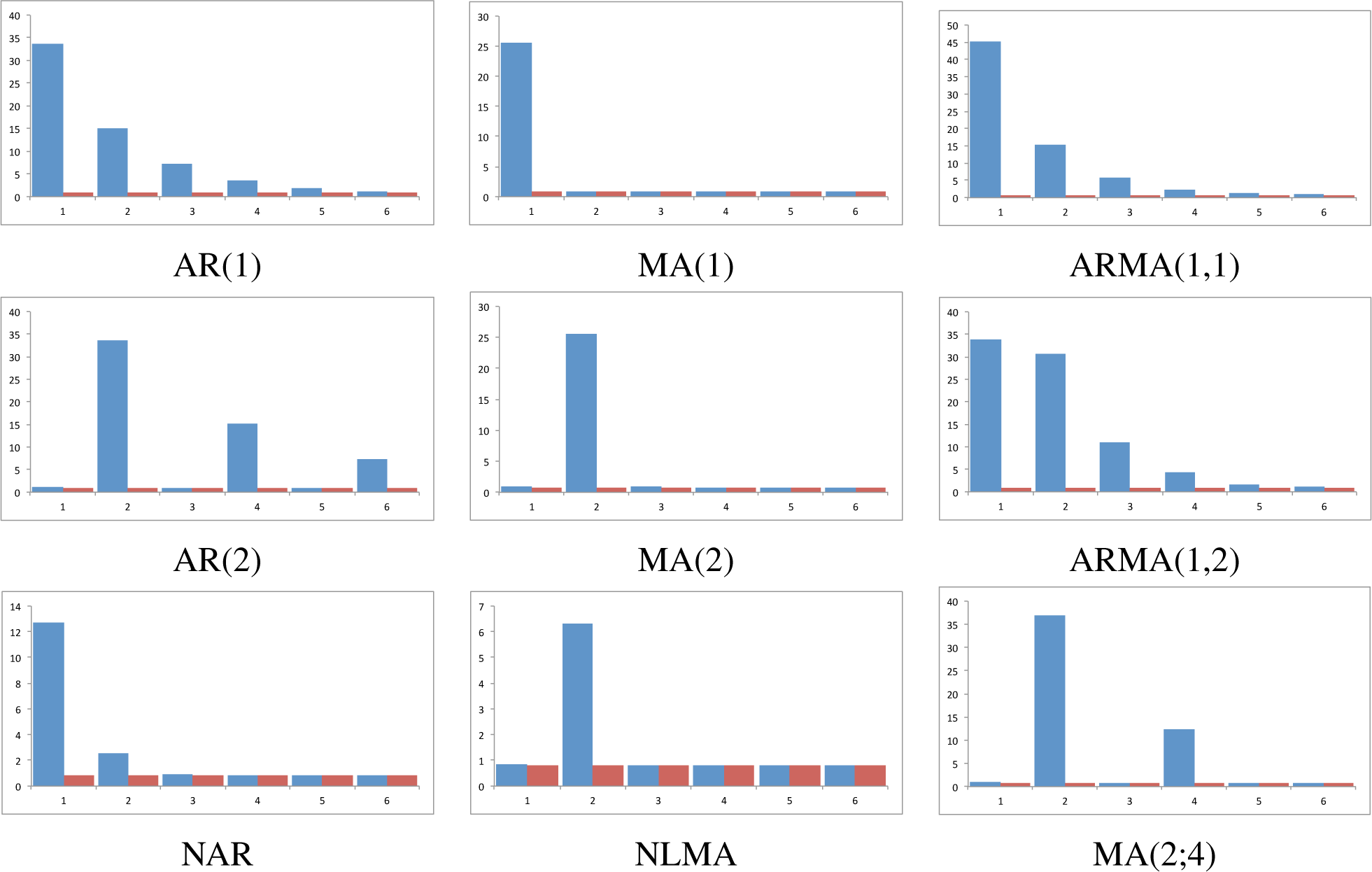
The shared characteristic of these models is that they all have a linear conditional mean. However, some are autoregressive, some moving averages of external shocks and some are mixture of linear processes. These models are well-known in univariate time series analysis, so for the statistic to be of some utility a clear detection of the lag and of the model is expected. Autoregressive models have memory, while moving average models do not. Accordingly, this essential difference should be detected. 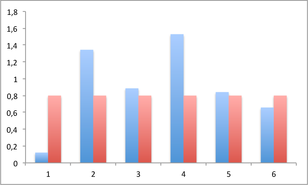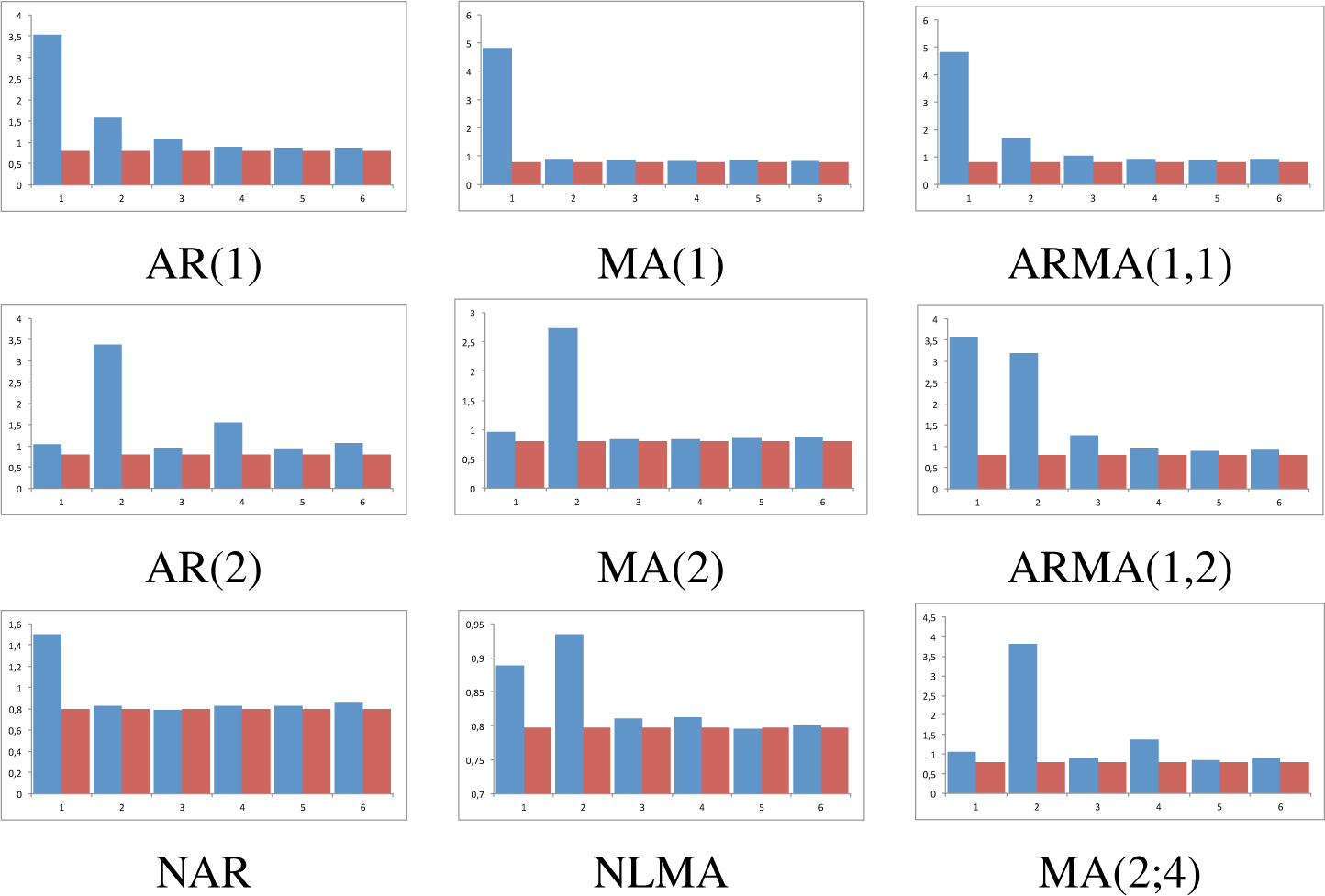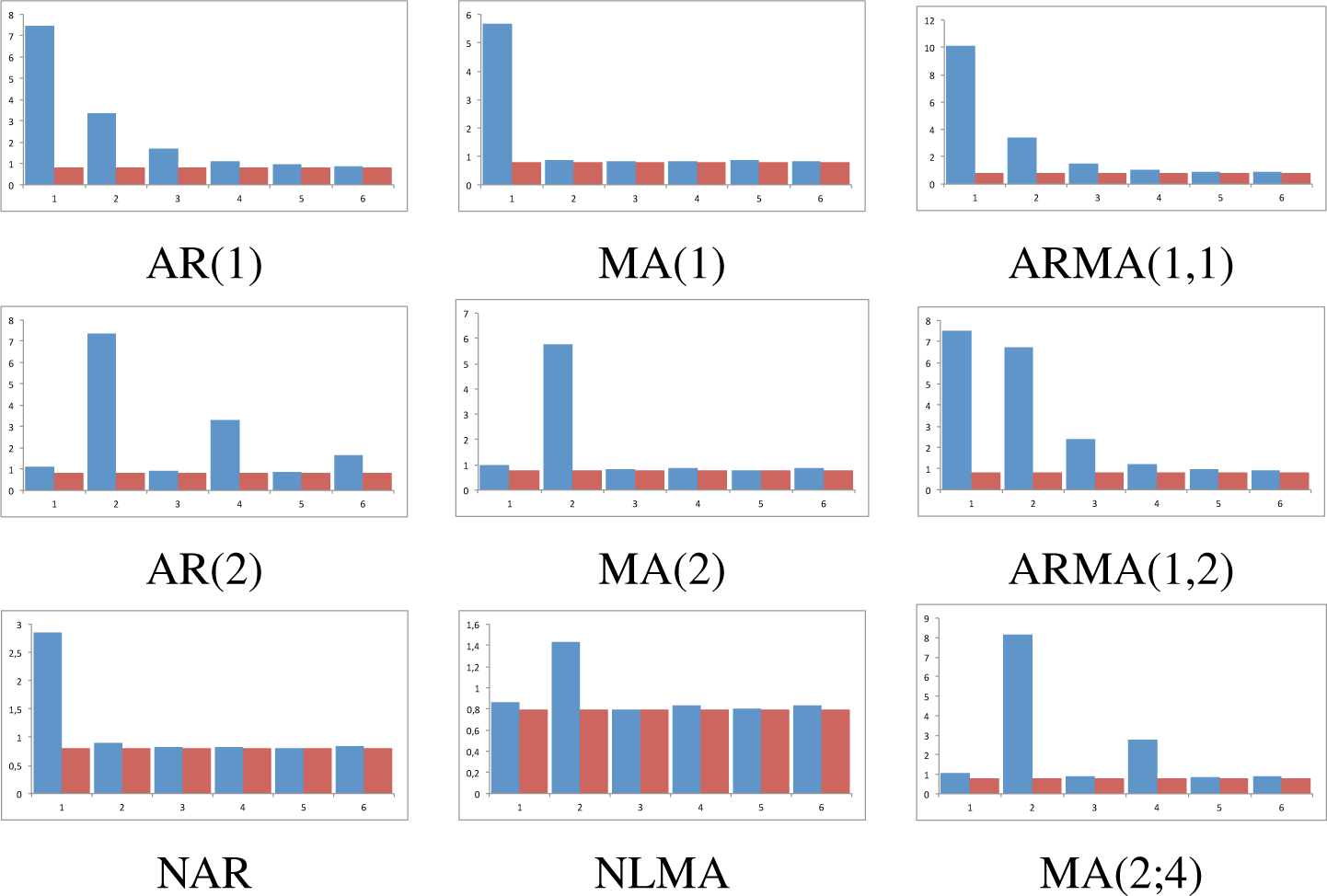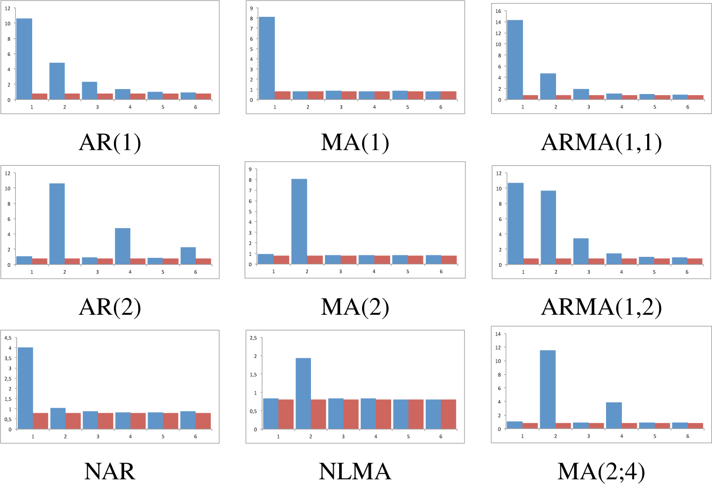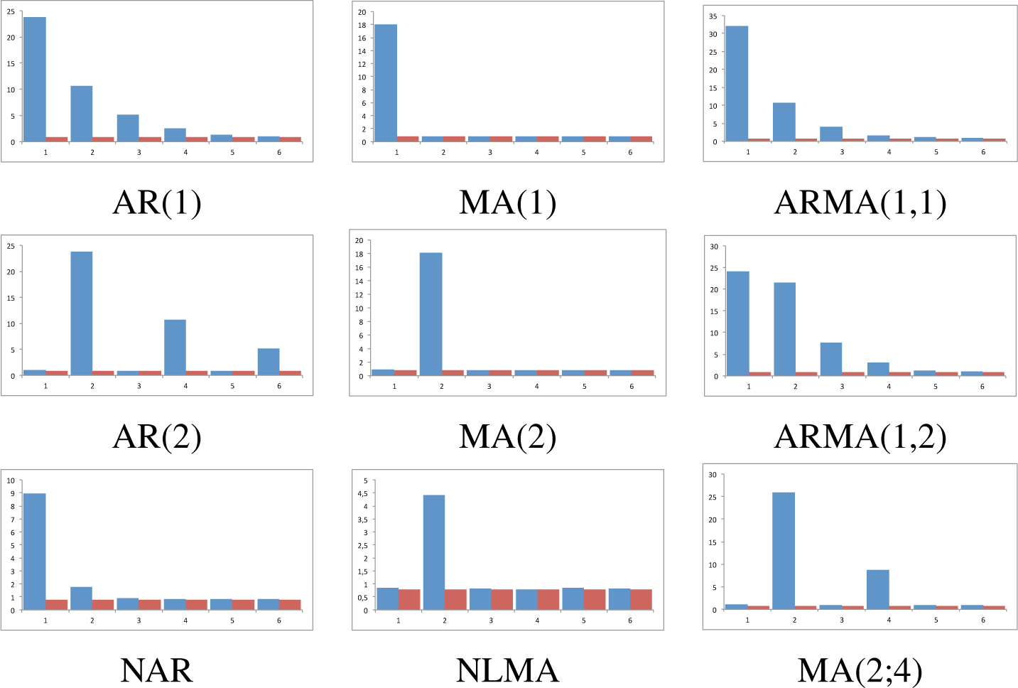We compute the average value of the ${\mathrm{\Lambda }}_3^p$ statistic for sample sizes n = 120, 360, 500, 1000, 5000, 10000 of 1000 Monte Carlo simulations for the seven models. We also do the same for a benchmark normal (0,1) model, which is an i.i.d. process and allows us to show if the expected value of $E({\mathrm{\Lambda }}_q^p)=\sqrt{\frac{2}{\pi }}\approx 0.7979$. is achieved empirically. Averages are given in Figure 1, that reports the results for the largest sample size; while the behavior for the remaining sample sizes are given in Figures 4–8 which can be found in the appendix.

For models AR(1) and AR(2) the statistic clearly shows an exponential decrease in ${\mathrm{\Lambda }}_3^p$, indicating (a) that the correct lag is in 1 and 2, respectively; (b) that the data generating process has memory respecting the true lag, as each true lag is less relevant that the preceding one; and (c) this occurs for all sample sizes. Interestingly, observation (b) sharply contrast with classical techniques that do not gather this salient empirical fact. For models MA(1) and MA(2), our statistic also performs as expected for identifying the model: the true lag is detected, the memoryless basic property is clearly observed for all lags, and therefore cannot be confused with an AR(p) model. The results for mixed models are also of interest. Regarding the ARMA(1,1), the statistic reaches its maximum at the correct lag, namely, 1, and then decays exponentially to zero; given the MA structure at lag 1, statistic’s decay from its value at lag 1 and 2 is more prominent than in the case of an AR(1). This can also be devised for ARMA(1,2) model: the two relevant lags are clearly detected, namely, 1 and 2; the statistic does not decay very fast at lag 2 given its MA(2) structure, but it reappears for p > 2. Finally, in the MA(2;4) model, we have considered a moving average linear process with different weights in the two relevant lags, so we expect and observe that the proposed statistic firstly estimates the correct lag and then determines its relevance. To complete the analysis, the results are compared for two non linear models previously studied (DGP 2 and DGP 3), which are nonlinear counterparts of AR and MA models. It can be observed that the exponential decaying behavior is much faster in the nonlinear case than in the linear case, for the autoregressive models. For the moving average models, the values of the statistic, while being statistically significant, are lower than in the linear MA counterpart.

We now illustrate how our tools can be used for helping in the modelling process of real data. To this end we have considered a well-known empirical time series, namely, the returns obtained from closing values of the daily New York Stock Exchange (NYSE) index from 2000 to 2008 (Figure 2).

Given the series of returns, our proposal consists of using the tools previously presented. To this end we compute ${\mathrm{\Lambda }}_3^p$ for several lags for the selected time series. The results are given in Figure 3. According to the results, our statistical procedure identifies lags 2 and 4, so the modeler is recommended to use these two lags. As regarding the identification of the underlying model, in view of the Figure 3 when compared with Figure 2, it does not seem that the model is of an autoregressive linear nature, and seem to be closer to a moving average process where lags 2 and 4 will play a relevant role.

6. Conclusions

In this paper, we have presented a statistical procedure, based on the distribution of symbols (number of runs), to estimate the relevant lag of a dynamic generating process from which the researcher only has one observed sample. This is the first time runs has been used for detecting structure, and it is also the first time it is used for model identification. The technique shows several appealing advantages: (1) It is model independent, so that the end-user can easily use it without assuming or estimating a model; (2) It can be used for stochastic processes of linear or nonlinear nature, because in both studied scenarios the procedure is very competitive and robust; (3) In the studied models, it correctly detects the correct lag even in the case of a relatively small number observations, which facilitates its use even in sciences where there are small samples; (4) When it is compared with the standard autocorrelation function and/or partial autocorrelation functions, the empirical results are undoubtedly in favor of the new statistical tool; and when compared with permutation entropy based procedures, it generally has more statistical power; (5) Particularly interesting for financial data analysis, it shows an extraordinary empirical behavior when the lag structure is in the second conditional moment of the data generating process; (6) It can be used for identifying, no only lags, but also linear models. Points (1) to (6) makes the new statistical tool general, and widely applicable for data analyzers.

References

1. Granger, C.; Weiss, A. Time Series Analysis of Error-Correcting Models. In Studies in Econometrics, Time Series, and Multivariate Statistics; Academic Press: New York, NY, USA, 1983. [Google Scholar]
2. Tjostheim, D. Measures and tests of independence: A survey. Statistics 1996, 28, 249–284. [Google Scholar]
3. Granger, C.; Lin, J. Using the mutual information coefficient to identify lags in nonlinear models. J. Time Series Anal. 1994, 15, 371–384. [Google Scholar]
4. Tjostheim, D.; Auestad, B. Nonparametric identification of nonlinear time series: Selecting significant lags. J. Am. Statist. Assoc. 1994, 89, 1410–1419. [Google Scholar]
5. Matilla-Garcia, M.; Ruiz Marin, M. Detection of non-linear structure in time series. Econ. Lett. 2009, 105, 1–6. [Google Scholar]
6. Zunino, L.; Soriano, M.C.; Fischer, I.; Rosso, O.A.; Mirasso, C.R. Permutation-information-theory approach to unveil delay dynamics from time-series analysis. Phys. Rev. E 2010, 82, 046212. [Google Scholar]
7. Soriano, M.C.; Zunino, L.; Rosso, O.A.; Fischer, I.; Mirasso, C.R. Time Scales of a Chaotic Semiconductor Laser with Optical Feedback Under the Lens of a Permutation Information Analysis. IEEE J. Quant. Electr. 2011, 42, 242–261. [Google Scholar]
8. Toomey, J.P.; Kane, D.M. Mapping the dynamic complexity of a semiconductor laser with optical feedback using permutation entropy. Opt. Express 2014, 22, 1713–1725. [Google Scholar]
9. Amigo, J.M. Permutation Complexity in Dynamical Systems; Springer: Berlin, Germany, 2010. [Google Scholar]
10. Shannon, C.E.; Weaver, W. The Mathematical Theory of Communication; University of Illinois Press: Urbana, IL, USA, 1949. [Google Scholar]
11. Morse, M. Recursive geodesic on a surface of negative curvature. Trans. Am. Math. Soc. 1949, 22, 84–100. [Google Scholar]
12. Collet, P.; Eckmann, J.P. Iterated Maps on the Interval as Dynamical Systems; Brickhauser: Basel, Switzerland, 1980. [Google Scholar]
13. Ruiz Marin, M.; Faura, U.; Lafuente, M.; Dore, M. H. I. Nonparametric Tests for Serial Dependence Based on Runs. Dyn. Psychol. Life Sci. 2014, 18, 123–136. [Google Scholar]
Figure 1. Mean value of Λ 3 p statistic as a function of the lag time (for p = 1, 2,…, 6). Sample size for each realization is fixed at n = 10,000. The number of Monte Carlo simulations is 1000 for each model. Blue bars refer to average the Λ 3 p for each model. Red bars refer to the benchmark iid process.
Entropy 17 02706f1
Figure 2. NYSE Daily Returns (2000–2008).
Entropy 17 02706f2
Figure 3. Λ 3 p function for NYSE Daily Returns (blue) and (red) expected value for Λ 3 p in case of no relevant lag.
Entropy 17 02706f3