
Entropy, Information and Complexity or Which Aims the Arrow of Time?

Abstract
:1. Introduction
2. Entropy, Information, Complexity and Time
2.1. Entropy, the Boltzmann H-Theorem and His Formula
2.2. Information, Shannon Formula and Its Similarity with the Boltzmann One
2.3. Interpretation Entropy as Information
2.4. Algorithmic Complexity and Its Similarity to Entropy
3. Non-Statistical Approach to the Definition of Generalized Entropy, Using the Theory of Categories and Functors
3.1. Category Theory as a Language for Describing a Wide Variety of Systems
3.2. Formulation of the Generalized Entropy for Categories Applicable to Any System Described by These Mathematical Structures
3.3. Competition for Resources and Metabolic Time
3.4. Extremal Principle as a Law of System Variability, Its Entropy and Information Interpretation and the Irreversibility of Time Generated by It
- It is far more probable to find a system in a complex state than in a simple one.
- If a system came to a simple state, the probability that the next state will be simpler is immeasurably less than the probability that the next state will be more complicated.
4. Law Defining the Arrow of Time and Its Direction
4.1. General Law of Complification
Any natural process in a dynamic system leads to an irreversible and inevitable increase in its algorithmic complexity, together with an increase in its generalized entropy and information.
4.2. Place of General Law of Complification among the Other Laws of Nature
4.3. Hierarchical Forces and the Third Unique Feature of the General Law of Complification
4.4. Two Worlds: Large, Complex and Irreversible and Small, Simple and Timeless
5. Evolution of the Universe, Its Engine and Its Driver
5.1. Diversity and Selection in Physical-Chemical Evolution and Laws of Nature as “Breeder”
5.2. Evolution in a Steady Stream of Free Energy, Dissipative Structures and Their Selection
5.3. Biological Evolution of Dissipative Structures and the Role of Catastrophes, Natural and Artificial, in It
6. Conclusions
- The irreversibility of time is expressed as the increase in entropy, information, degrees of freedom and complexity, which rise monotonically with respect to each other.
- Using the extremal principle and theory of categories, it was shown that the entropy of the system can be determined without any statistical assumptions and distributions as a generalized entropy and, consequently, information, degrees of freedom and complexity.
- The increase in such generalized entropy, information, degrees of freedom and complexity can be considered as a generalization of the second law of thermodynamics in the form of the general law of complification and determines the direction of the arrow of time in our universe.
- The engine of physicochemical evolution (as the implementation of the arrow of time) is the general law of complification, while its driver is the other laws of nature, which are very simple and exist essentially out of time.
- The mechanism of physicochemical evolution is eliminating or stabilizing selection of structures admissible by the laws of nature (i.e., stable) from the entire set of options generated by complification.
- The emergence of stars, generated by the steady stream of free energy, allowed selecting not only stable, but also dissipative structures, competing for energy and material resources and maximizing entropy production.
- The enrichment of selection with competition for resources and the survival of not just possible, but the fittest structures elevated evolution to the new, biological level, and this biological evolution was accelerated sharply, especially due to managing internal catastrophes by multicellular organisms.
- Thus, the flight of the arrow of time constantly accelerates, and its aim is maximum at the moment of the complexity, degrees of freedom, information and entropy. However, this arrow never hits local targets, because of the limitations imposed by the laws of nature and, in particular, by catastrophes.
Acknowledgments
Author Contributions
Conflicts of Interest
References
- Boltzmann, L. Weitere Studien Uber das Warmegleichgewicht Unter Gas Molekulen; Springer: Wiesbaden, Germany, 1970. [Google Scholar]
- Shannon, C.E.; Weaver, W. The Mathematical Theory of Communication; University of Illinois Press: Urbana, IL, USA, 1963. [Google Scholar]
- McArthur, R. On the Relative Abundance of Species. Am. Nat. 1960, 94, 25–36. [Google Scholar]
- Hutcheson, K. A Test for Comparing Diversities Index Based on Shannon Formula. J. Theor. Biol. 1970, 29, 151–154. [Google Scholar]
- Wiener, N. Cybernetics, or the Control and Communication in the Animal and the Machine, 2nd ed.; The MIT Press: Cambridge, MA, USA, 1965. [Google Scholar]
- Eco, U. Opera Aperta: Forma e Indeterminazione nelle Poetiche contemporanee; Bompiani: Milano, Italy, 2011. [Google Scholar]
- Brillouin, L. La Science et la Theorie de l’Information; Editions Jacques Gabay: Paris, France, 1988. [Google Scholar]
- Ben-Naim, A. Entropy and the Second Law: Interpretation and Miss-interpretations; World Scientific: Singapore, Singapore, 2012. [Google Scholar]
- Ben-Naim, A. Entropy Demystified; World Scientific: Singapore, Singapore, 2008. [Google Scholar]
- Gell-Mann, M. The Quark and the Jaguar, 3rd ed.; St. Martin’s Press: London, UK,, 1995. [Google Scholar]
- Lloyd, S. Measures of Complexity: A Non-exhaustive List. IEEE Control Syst. Mag. 2001, 21, 7–8. [Google Scholar]
- Solomonoff, R.J. A Formal Theory of Inductive Inference. Part I. Inf. Control. 1964, 7, 1–22. [Google Scholar]
- Solomonoff, R.J. A Formal Theory of Inductive Inference. Part II. Inf. Control. 1964, 7, 224–254. [Google Scholar]
- Kolmogorov, A.N. Three Approaches to the Quantitative Definition of Information. Probl. Inf. Transm. 1965, 1, 1–7. [Google Scholar]
- Chaitin, G.J. On the Length of Programs for Computing Finite Binary Sequences: Statistical Considerations. J. Assoc. Comput. Mach. 1969, 16, 145–159. [Google Scholar]
- Kolmogorov, A.N. Combinatorial Foundations of Information Theory and the Calculus of Probabilities. Russ. Math. Surv. 1983, 38, 29–40. [Google Scholar]
- Cover, P.; Gacs, T.M.; Gray, R.M. Kolmogorov’s Contributions to Information Theory and Algorithmic Complexity. Ann. Probab. 1989, 17, 840–865. [Google Scholar]
- Lloyd, S.; Pagels, H. Complexity as Thermodynamic Depth. Ann. Phys. 1988, 188, 186–213. [Google Scholar]
- Febres, G.; Jaffe, K. A Fundamental Scale of Descriptions for Analyzing Information Content of Communication Systems. Entropy 2015, 17, 1606–1633. [Google Scholar]
- Grunwald, P.; Vitanyi, P. Shannon Information and Kolmogorov Complexity 2004, arXiv, cs/0410002.
- Ladyman, J.; Lambert, J.; Weisner, K.B. What is a Complex System? Eur. J. Philos. Sci. 2013, 3, 33–67. [Google Scholar]
- Lloyd, S. On the Spontaneous Generation of Complexity in the Universe. In Complexity and the Arrow of Time; Lineweaver, C.H., Davis, P.C.W., Ruse, M., Eds.; Cambridge University Press: Cambridge, UK, 2013; pp. 80–112. [Google Scholar]
- Sant’Anna, A.S. Entropy is Complexity 2004, arXiv, math-ph/0408040.
- Teixeira, A.; Matos, A.; Souto, A.; Antunes, L. Entropy Measures vs. Kolmogorov Complexity. Entropy 2011, 13, 595–611. [Google Scholar]
- Wolpert, D.H. Information Width: A Way for the Second Law to Increase Complexity. In Complexity and the Arrow of Time; Lineweaver, C.H., Davis, P.C.W., Ruse, M., Eds.; Cambridge University Press: Cambridge, UK, 2013; pp. 246–275. [Google Scholar]
- Levich, A.P. Time as Variability of Natural Systems. In On the Way to Understanding the Time Phenomenon: The Constructions of Time in Natural Science, Part 1; World Scientific: Singapore, Singapore, 1995; pp. 149–192. [Google Scholar]
- Levich, A.P.; Solov’yov, A.V. Category-Functor Modelling of Natural Systems. Cybern. Syst. 1999, 30, 571–585. [Google Scholar]
- Levich, A.P. Art and Method of Systems Modeling: Variational Methods in Communities Ecology, Structural and Extremal Principles, Categories and Functors; Computing Investigation Institute: Moscow, Russia, 2012. [Google Scholar]
- Levich, A.P.; Fursova, P.V. Problems and Theorems of Variational Modeling in Ecology of Communities. Fundam. Appl. Math. 2002, 8, 1035–1045. [Google Scholar]
- Kauffman, S.A. Evolution beyond Newton, Darwin, and Entailing Law: The Origin of Complexity in the Evolving Biosphere. In Complexity and the Arrow of Time; Lineweaver, C.H., Davis, P.C.W., Ruse, M., Eds.; Cambridge University Press: Cambridge, UK, 2013; pp. 162–190. [Google Scholar]
- Levich, A.P. Entropic Parameterization of Time in General Systems Theory. In Systems Approach in Modern Science; Progress-Tradition: Moscow, Russia, 2004; pp. 153–188. [Google Scholar]
- Eddington, A.S. The Nature of the Physical World: Gifford Lectures 1927; Cambridge University Press: Cambridge, UK, 2012. [Google Scholar]
- Tribus, M.; McIrvine, E.C. Energy and Information. Sci. Am. 1971, 225, 179–188. [Google Scholar]
- Cooper, L.N. An Introduction to the Meaning and Structure of Physics; Harper: New York, NY, USA, 1968. [Google Scholar]
- Goldreich, O. P, NP, and NP-Completeness: The Basics of Computational Complexity; Cambridge University Press: Cambridge, UK, 2010. [Google Scholar]
- Fuentes, M.A. Complexity and the Emergence of Physical Properties. Entropy 2014, 16, 4489–4496. [Google Scholar]
- Lineweaver, C.H. A Simple Treatment of Complexity : Cosmological Entropic Boundary Conditions on Increasing Complexity. In Complexity and the Arrow of Time; Lineweaver, C.H., Davis, P.C.W., Ruse, M., Eds.; Cambridge University Press: Cambridge, UK, 2013; pp. 42–67. [Google Scholar]
- Lloyd, S. Black Holes, Demons and the Loss of Coherence: How Complex Systems Get Information, and What They Do with It. Ph.D. Thesis, The Rockefeller University, NY, USA, April 1988. [Google Scholar]
- Wolchover, N. New Quantum Theory Could Explain the Flow of Time. 2014. Available online: http://www.wired.com/2014/04/quantum-theory-flow-time/ accessed on 8 July 2015.
- Wolchover, N. February 1927: Heisenberg’s uncertainty principle. Am. Phys. Soc. News. 2008, 17, 3. [Google Scholar]
- Mikhailovsky, G.E. Biological Time, Its Organization, Hierarchy and Presentation by Complex Values. In On the Way to Understanding the Time Phenomenon: The Constructions of Time in Natural Science, Part 1; Levich, A.P., Ed.; World Scientific: Singapore, Singapore, 1995; pp. 68–84. [Google Scholar]
- Mikhailovsky, G.E. Organization of Time in Biological Systems. J. Gen. Biol. 1989, 50, 72–81. [Google Scholar]
- Auletta, G.; Ellis, G.F.R.; Jaeger, L. Top-down Causation by Information Control: From a Philosophical Problem to a Scientific Research Program. J. R. Soc. Interface. 2008, 5, 1159–1172. [Google Scholar]
- Ellis, G. Recognizing Top-Down Causation. In Questioning the Foundations of Physics; Springer: Berlin, Germany, 2013; pp. 17–44. [Google Scholar]
- Prigogine, I. From Being to Becoming: Time and Complexity in the Physical Sciences; W.H. Freeman & Co: San Francisco, CA, USA, 1980. [Google Scholar]
- Shulman, M. Kh. Entropy and Evolution. 2013. Available online: http://www.timeorigin21.narod.ru/eng_time/Entropy_and_evolution_eng.pdf accessed on 8 July 2015.
- Wigner, E.P. The Unreasonable Effectiveness of Mathematics in the Natural Sciences. Richard Courant Lecture in Mathematical Sciences Delivered at New York University, May 11, 1959. Commun. Pure Appl. Math. 1960, 13, 1–14. [Google Scholar]
- Yanofsky, N.S. Outer Limits of Reason: What Science, Mathematics, and Logic Cannot Tell Us; The MIT Press: Cambridge, MA, USA, 2013; p. 403. [Google Scholar]
- Thomson, W. On the Dynamical Theory of Heat. Trans. R. Soc. EdinburghExcerpts 1851, §§1. [Google Scholar]
- Penzias, A.A.; Wilson, R.W. A Measurement of Excess Antenna Temperature at 4080 Mc/s. Astrophys. J 1965, 142, 419–421. [Google Scholar]
- Freedman, W.L. Theoretical Overview of Cosmic Microwave Background Anisotropy. In Measuring and Modeling the Universe; Cambridge University Press: Cambridge, UK, 2004; pp. 291–309. [Google Scholar]
- Newton, I. Philosophiae Naturalis Principia Mathematica; Royal Society: London, UK, 1684. [Google Scholar]
- Liddle, A.R.; Lyth, D.H. Cosmological Inflation and Large-scale Structure; Cambridge University Press: Cambridge, UK, 2000. [Google Scholar]
- Mukhanov, V. Physical Foundations of Cosmology; Cambridge University Press: Cambridge, UK, 2005. [Google Scholar]
- Lloyd, S. Computational Capacity of the Universe. Phys. Rev. Lett. 2002, 88, 237901. [Google Scholar]
- Charlesworth, B. Stabilizing Selection, Purifying Selection, Mutational Bias in Finite Populations. Genetics 2013, 194, 955–971. [Google Scholar]
- Martyushev, L.M. Entropy and Entropy Production: Old MMisconceptions and New Breakthroughs. Entropy 2013, 15, 1152–1170. [Google Scholar]
- Martyushev, L.M.; Zubarev, S.M. Entropy Production of Main-Sequence Stars. Entropy 2015, 17, 658–668. [Google Scholar]
- Prigogine, I. Time, structure and fluctuations Nobel lecture. 1977, 23.
- Zeigler, H. Some Extremum Principles in Irreversible Thermodynamics with Application to Continuum Mechanics; Swiss Federal Institute of Technology: Lausanne, Switzerland, 1962. [Google Scholar]
- Prigogine, I. Introduction to Thermodynamics of Irreversible Processes; Interscience: New York, NY, USA, 1961. [Google Scholar]
- Haken, H. Information and Self-organization: A Macroscopic Approach to Complex Systems; Springer: Berlin, Germany, 2006. [Google Scholar]
- Nicolis, G.; Prigogine, I. Self-organization in Nonequilibrium Systems: From Dissipative Structures to Order through Fluctuations; Wiley: Hoboken, NJ, USA, 1977. [Google Scholar]
- Sharov, A.A.; Gordon, R. Life before Earth 2013, arXiv, 1304.3381.
- Demetrius, L.A.; Gundlach, V.M. Directionality Theory and the Entropic Principle of Natural Selection. Entropy 2014, 16, 5428–5522. [Google Scholar]
- Kauffman, S. The Emergence of Autonomous Agents. In From Complexity to Life (on the Emergence of Life and Meaning); Gregersen, N.H., Ed.; Oxford University Press: Oxford, UK, 2003; pp. 47–71. [Google Scholar]


| High-ordered Sates | Low-ordered States |
|---|---|
| Entropy is low | Entropy is high |
| Information is low | Information is high |
| Order | Chaos/Disorder |
| Simplicity | Complexity |
| Uniformity | Diversity |
| Subordination | Freedom |
| Rigidity | Ductility |
| Structuring | Randomization |
| Lattice | Tangle |
| Predictive | Counterintuitive |
| Manageability (direct) | Unmanageability/indirect control |
| Immaturity (for ecosystems) | Climax (for ecosystems) |
| Agrocenoses | Wild biocenoses |
| Dictatorship (for society) | Democracy (for society) |
| Planned economy | Free market |
| Mono-context | Poly-context |
| Poor synonym language | Rich synonym language |
| Artificiality | Naturalness |
| Degradation | Diversification |
| Code | Language |
| Army | Civil society |
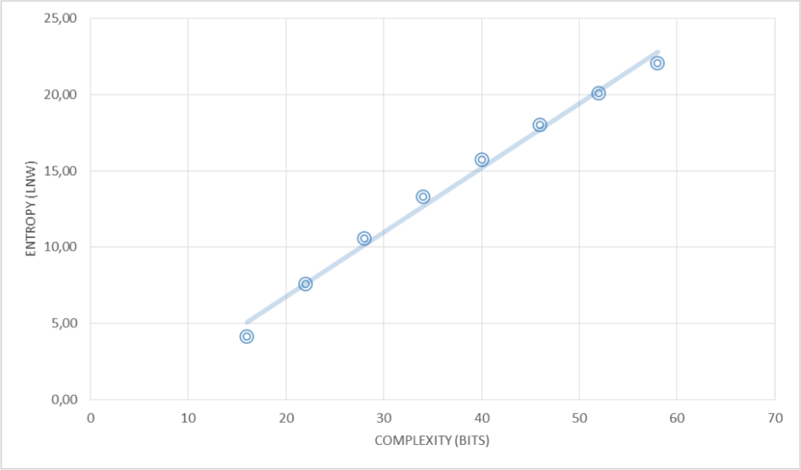
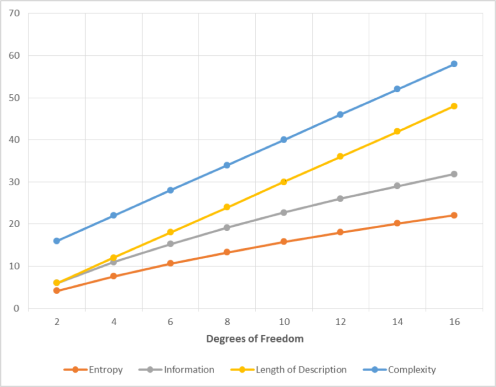
| Degrees of Freedom | W (cumulative) | W | Entropy S = lnW | Information I = log2W | Length of Description (D) | Complexity (D + Program) | |
|---|---|---|---|---|---|---|---|
| 2 | 64 | 64 | 4.16 | 6.00 | 6 | 16 | |
| 4 | 2016 | 1952 | 619.50 | 7.58 | 10.93 | 12 | 22 |
| 6 | 41,664 | 39,648 | 304.16 | 10.59 | 15.27 | 18 | 28 |
| 8 | 635,376 | 593,712 | 176.28 | 13.29 | 19.18 | 24 | 34 |
| 10 | 7,624,512 | 6,989,136 | 113.44 | 15.76 | 22.74 | 30 | 40 |
| 12 | 74,974,368 | 67,349,856 | 78.16 | 18.03 | 26.01 | 36 | 46 |
| 14 | 621,216,192 | 546,241,824 | 56.50 | 20.12 | 29.02 | 42 | 52 |
| 16 | 4,426,165,368 | 3,804,949,176 | 22.06 | 31.83 | 48 | 58 |
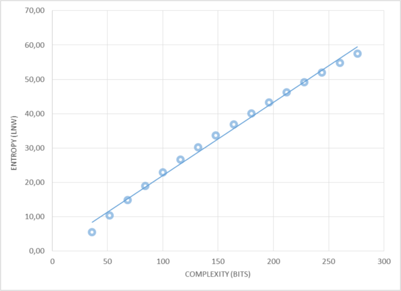
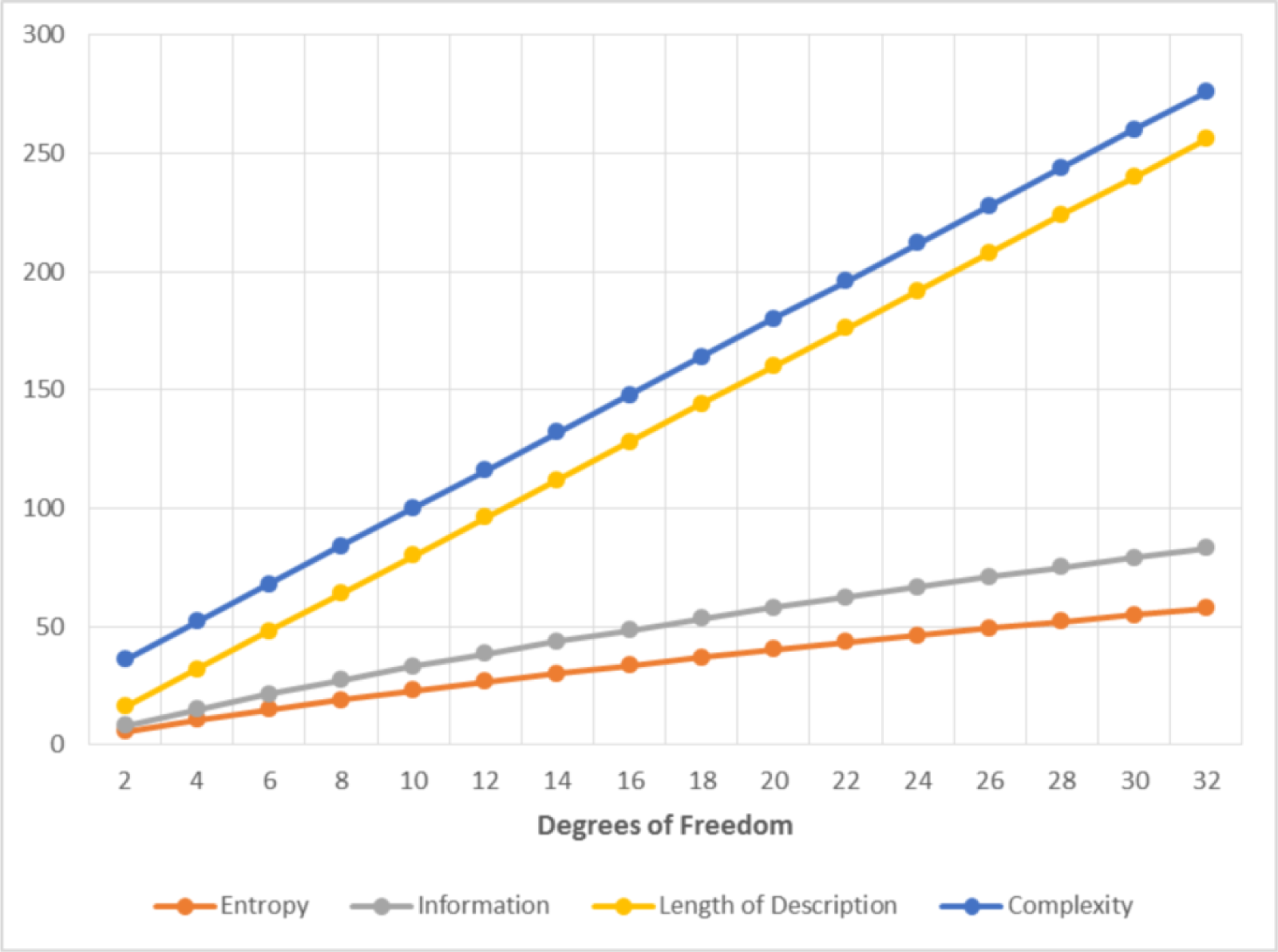
| Degrees of Freedom | W (cumulative) | W | Entropy S = lnW | Information I = log2W | Length of Description (D) | Complexity (D + Program) | |
|---|---|---|---|---|---|---|---|
| 2 | 256 | 256 | 5.55 | 8.00 | 16 | 36 | |
| 4 | 32,640 | 32,384 | 10,667.50 | 10.39 | 14.98 | 32 | 52 |
| 6 | 2,763,520 | 2,730,880 | 5,312.16 | 14.82 | 21.38 | 48 | 68 |
| 8 | 174,792,640 | 172,029,120 | 3,161.90 | 18.96 | 27.36 | 64 | 84 |
| 10 | 8,809,549,056 | 8,634,756,416 | 2,091.06 | 22.88 | 33.01 | 80 | 100 |
| 12 | 368,532,802,176 | 359,723,253,120 | 1,481.61 | 26.61 | 38.39 | 96 | 116 |
| 14 | 13,161,885,792,000 | 12,793,352,989,824 | 1,102.24 | 30.18 | 43.54 | 112 | 132 |
| 16 | 409,663,695,276,000 | 396,501,809,484,000 | 850.35 | 33.61 | 48.49 | 128 | 148 |
| 18 | 11,288,510,714,272,000 | 10,878,847,018,996,000 | 674.75 | 36.93 | 53.27 | 144 | 164 |
| 20 | 278,826,214,642,518,000 | 267,537,703,928,246,000 | 547.55 | 40.13 | 57.89 | 160 | 180 |
| 22 | 6,235,568,072,914,500,000 | 5,956,741,858,271,980,000 | 452.55 | 43.23 | 62.37 | 176 | 196 |
| 24 | 127,309,514,822,004,000,000 | 121,073,946,749,089,000,000 | 379.77 | 46.24 | 66.71 | 192 | 212 |
| 26 | 2,389,501,662,813,000,000,000 | 2,262,192,147,991,000,000,000 | 322.82 | 49.17 | 70.94 | 208 | 228 |
| 28 | 41,474,921,718,825,700,000,000 | 39,085,420,056,012,700,000,000 | 277.45 | 52.02 | 75.05 | 224 | 244 |
| 30 | 669,128,737,063,722,000,000,000 | 627,653,815,344,896,000,000,000 | 240.75 | 54.80 | 79.05 | 240 | 260 |
| 32 | 10,078,751,602,022,300,000,000,000 | 9,409,622,864,958,580,000,000,000 | 57.50 | 82.96 | 256 | 276 |
© 2015 by the authors; licensee MDPI, Basel, Switzerland This article is an open access article distributed under the terms and conditions of the Creative Commons Attribution license (http://creativecommons.org/licenses/by/4.0/).
Share and Cite
Mikhailovsky, G.E.; Levich, A.P. Entropy, Information and Complexity or Which Aims the Arrow of Time? Entropy 2015, 17, 4863-4890. https://0-doi-org.brum.beds.ac.uk/10.3390/e17074863
Mikhailovsky GE, Levich AP. Entropy, Information and Complexity or Which Aims the Arrow of Time? Entropy. 2015; 17(7):4863-4890. https://0-doi-org.brum.beds.ac.uk/10.3390/e17074863
Chicago/Turabian StyleMikhailovsky, George E., and Alexander P. Levich. 2015. "Entropy, Information and Complexity or Which Aims the Arrow of Time?" Entropy 17, no. 7: 4863-4890. https://0-doi-org.brum.beds.ac.uk/10.3390/e17074863