1. Introduction
The goal of a probabilistic seismic hazard analysis (PSHA) is to quantify the rate of exceeding various ground motion levels at a site, given all possible earthquakes. Therefore, PSHA is a methodology that estimates the likelihood that various levels of earthquake-caused ground motions will be exceeded at a given location in a given future time period. The results are expressed as estimated probabilities per unit of time or estimated frequencies [
1].
Milne and Davenport [
2] developed an empirical statistical method. However, this method has been replaced by the numerical models initiated by Cornell [
3]. The most complete information about PSHA can be found in the Senior Seismic Hazard Analysis Committee report [
1].
A key point in order to do a PSHA is to define the geometry of the seismic sources. This is depicting the seismic zones in a map and representing the locations within the Earth’s crust that have uniform seismicity characteristics.
A seismic source is a region that has relatively uniform seismic characteristics, and it is different from neighboring sources. It is possible to allow for some variation of a- and b-values within a given seismic source. Nevertheless, the maximum magnitude and the earthquake recurrence are assumed to be uniform.
Modern PSHA mainly considers two kinds of seismic sources: seismogenic zones and large faults. In modern PSHA, both models are applied together, forming hybrid models. Up to a threshold magnitude, seismic occurrence is dominated by zones and, for larger earthquakes, by main faults.
The geometry of seismic sources is the aspect of PSHA that depends more on the earthquake environment considered. In high-activity regions, the locations and geometries of seismic sources (faults) are less uncertain than their recurrence rates. The recurrence rates are normally based on geologic data. In low-activity regions (normally of small to moderate magnitude earthquakes), the geometry of the seismic sources is often highly uncertain (area sources). The recurrence rates are obtained from seismic data.
Fault sources must be plotted in a map. The intersection of shallow faults with the ground surface is depicted in a fault map. The shallowest extent of blind surfaces must be also drawn in the map. Relevant faults are main faults with quaternary activity evidence.
Contrariwise, for small to moderate earthquake magnitude zones, it is difficult to identify faults. Due to this, area sources have been conceived of for PSHA. These are a simplified representation of one or more seismogenic structures whose location is unknown [
1]. Area sources are defined by their boundaries depicted on a map. These boundaries classify zones according to their maximum magnitude and recurrence rate. Area source boundaries can be defined by a variety of characteristics, including concentrations of seismicity and changes in tectonic and geologic boundaries. Moreover, it is also advisable to consider the depth distribution of seismicity to identify anomalous relative to other regions. Finally, the focal mechanism must be considered.
Seismogenic zones have traditionally been defined from the spatial distribution of seismic epicenters and shallow geological structures. This procedure is based on the available seismic database. In moderately active zones, the database can be incomplete. Likewise, the geological structures considered are not related to the current tectonic regime many times (paleogeographic criteria, pre-alpine structures, etc.). This has caused that the same area can have as many seismogenic zones as authors.
The analysis of the thermal and resistant parameters (thickness variations, pre-existing faults, thermal inhomogeneities, rheological inhomogeneities, constant temperature or constant heat flux, plain strain or plain stress models) of the crust provides a better criterion for the definition of the seismic sources, rather than correlation between epicenters and geologic structures. Nonetheless, there is great uncertainty in the construction of rheological profiles [
4].
Morales-Esteban
et al. [
5] studied the seismicity of the Iberian Peninsula (IP). They concluded that its seismicity is moderate, generally characterized by earthquakes less than 5.0. Large earthquakes happen after long periods of time. The seismicity is caused by the convergence between Eurasia and Africa’s plates, and it is spread over large areas. These characteristics make it necessary to define seismogenic zones before doing a PSHA.
The goal of this research is to introduce a new seismogenic zoning method. For that purpose, a computational technique based on triclustering, TriGen [
6,
7], has been applied. Triclustering mines 3D datasets in order to extract patterns of coherent behavior. TriGen is applied to data obtained from the catalog of the National Geographic Institute of Spain (NGIS), due to its ability to find compact areas regardless the spatial coordinates. Later, the obtained zones are correlated with the geology. This way, the bias is greatly eliminated, as the method is solely based on seismic data. Almost no human decision is made. The subsequent correlation with the geology is used to check the validity of the obtained zones. This method could be used in other areas of the world with similar tectonic characteristics (small to moderate earthquakes, individual faults that are hard to identify and spread seismicity).
The rest of the work is structured as follows. In Section 2, some related works regarding both the seismogenic zoning of the IP and the use of triclustering algorithms are described. Section 3 describes the seismicity of the Iberian Peninsula. In Section 4, a description of the methodology used to generate the seismogenic zoning of the Iberian Peninsula is detailed. Section 5 shows the results obtained. A comparison to another zoning method, Kohonen’s self-organizing maps, can be found in Section 6. In Section 7, a critical review of the method is provided. Finally, the conclusions can be found in Section 8.
3. Seismicity and Tectonics of the Iberian Peninsula
The IP (Spain, Portugal, Andorra and Gibraltar) is located in the Eurasian plate next to the contact with African’s plate. The seismicity is moderate [
5,
30], and it is associated with convergence between these plates. Likewise, it is distributed over a wide area of deformation, as expected in a continent-continent collision. Long recurrence periods separate large events [
31,
32]. Most earthquakes are at a shallow depth (
h < 40 km). However, there is a significant seismic activity at intermediate (40 <
h < 130 km) and greater depths (
h ≤ 650 km) [
33]. Historical seismicity studies report the occurrence of large earthquakes in the south of Iberia. Instrumental magnitudes larger than 5.5 have mostly occurred in the Gulf of Cadiz and north of Africa. The largest recent earthquake was the Gorringe Bank (1969,
Ms = 8.0), and the largest earthquake in the Gulf of Cadiz (1964) was of a magnitude 6.2 [
30].
The plate limit is not homogenous, with constant oceanic and continental areas in contact. There is a consistent N-S to NW-SE orientation of P axes that corresponds to the plate convergence direction. This coexists with E-W- to NE-SW-directed horizontal tension in the Betics, the Alboran Sea and northern Morocco. The area of contact between the IP and the northwest of Africa is the most complicated area. This area is surrounded on both sides by frequent seismic activity with very large earthquakes [
34]. Large earthquakes, such as the Lisbon 1531, 1755 and 1909 earthquakes, have happened in this area.
The regional seismicity is diffuse and is not clearly aligned with the current limit between the two plates [
35]. The seismic activity extends to far away inter-plate areas, such as the northeast and the center of the IP.
Great seismic activity is located in the east of the Gibraltar Arc. It is spread over a large area approximately 500 km wide, centered at the Alboran Sea. It contains parts of the southeast of Spain, the north of Morocco and Algeria [
36]. At the west of Gibraltar, most earthquakes happen in the southern coast of Portugal, in the surroundings of the limit between the Azores and Gibraltar plates. Other seismic sources include the northwest of Spain, southern Portugal and the Pyrenees. Earthquakes are infrequent in other locations. This seismicity happens over several geo-tectonic regions with different rheology and tectonics.
There are three main tectonic regimes at the IP: first, the Hercynian block, known as the Iberian Massif, inactive Variscan orogeny; second, the Atlantic continental margin off Portugal and Spain; and third, the Alpine young orogenic belts formed by the Pyrenean fold and the Betic foldchain.
The core of the IP consists of a Hercynian block, known as the Iberian Massif. It is formed by various pieces that were assembled to form the block. The external part of the orogeny is the Cantabrian Zone. This is just deformed in the upper crustal layers. Contrariwise, the west Asturian Leonese Zone and Central Iberian Zone layers are more deeply deformed and metamorphosed. These three zones are part of a terrane. The other two zones, Ossa-Morena and south Portugal, are two different terranes that have become fastened. The Iberian Massif was marginally affected by the Alpine deformation. It is formed by folded Paleozoic and Precambrian rocks partially covered by Mesozoic and Tertiary deposits to the east. Nonetheless, it outcrops through the Iberian Chain and the Catalonian Coastal Ranges.
The IP is delimited to the west by the continental boundary formed by the magma-poor opening of the Atlantic Ocean. It is a unique 100 km-wide zone of exhumed continental mantle.
The Alpine orogenic belts are formed with thickening crust. They are located in the old limit between the African and the Iberian plates (the Pyrenees), on the northeast of the Iberian Massif. Currently, it is located in the limit between Africa and the Iberia plates (the orogenic belt Betica-Riff-Tell), on the southeast of the Iberian Massif. The inner depressions of the Cenozoic extensive tectonic regime include the folded depressions in the lower areas of the Alpine belt (Ebro depression at the south of the Pyrenees and the Guadalquivir depression at the north of the Betica), the larger inner depressions of the Tajo and the Duero and, in a lesser number, the intra-orogenic depressions in both the Hercynian and Alpine regions. Farther away, an local-scale extensive tectonic regime is active in the western part of the Mediterranean Sea. It is located in the Liguro-Provencal depression, Valencia depression, the depression at the south of the Balearic Islands located in the east of the IP and the Alboran depression at the south of Iberia [
37].
The Alboran Sea is from the lower Pliocene and is located in the limit between Eurasia and Africa plates. It is especially relevant for the proper understanding of the collision between plates. The continental crust in the Alboran depression has become considerably thinner (15 km compared with over 35 km at the center of the Betica [
38,
39]). The transition between the Alboran depression and the Neogene oceanic crust to the east is gradual [
40]. The formation of the Alboran depression in a compressive stress regime can be explained by the elimination of the lower parts of the crust; nevertheless, the mechanism is still not clear.
4. Method
This section describes the methodology used to generate the seismogenic zoning of the Iberian Peninsula. In this sense, the features of the database used, as well as all information related to the catalog are introduced in Section 4.1. Section 4.2 describes the data processing carried out in this work. Finally, a brief description of the TriGen algorithm can be found in Section 4.3.
4.1. Data Description and Retrieval
The database used for this study is the catalog of the NGIS. From 1961, the NGIS has routinely calculated the magnitude of the earthquakes placed between 35°N to 44°N and 10°W to 5°E. It also produces weekly, monthly and definitive catalogs from 1981 until today.
It uses five different correlations for the estimation of the magnitudes:
Duration magnitude, MD(M − MS).
Surface-wave magnitude, mb,Lg(M-MS).
Body-wave magnitude, m
b(V-C) [
41].
Surface-wave magnitude, mb,Lg(L).
Moment magnitude, M
w [
42].
A thorough description of these correlations is shown in Morales-Esteban
et al. [
5]. The estimation of the magnitudes in the catalog is not homogenous, as the earthquakes before 1962 (
MD) were calculated using a different procedure. In order to work out the b-value from Equations (4) and (5), the database must be complete. To guarantee the completeness of the data, the analysis should only include earthquakes recorded after the year of completeness of the catalog. This is the year from which all of the earthquakes of a magnitude larger to or equal to the minimum magnitude have been recorded. The works in [
43,
44] point out that the year of completeness of the catalog is 1978 and that the minimum magnitude is 3.0. Only earthquakes from 1978 and onwards are used in this study. The surface-wave magnitude (m
b,
Lg, hereinafter M) has been used in this study.
The procedure used for the location of the epicenters is described in Mezcua
et al. [
45]. Older epicenters have been determined using isoseismal maps. Later, the application HYPO 71, based on the time of arrival of the seismic waves to the stations and a model of the crust, has been used.
4.3. Description of the TriGen Algorithm
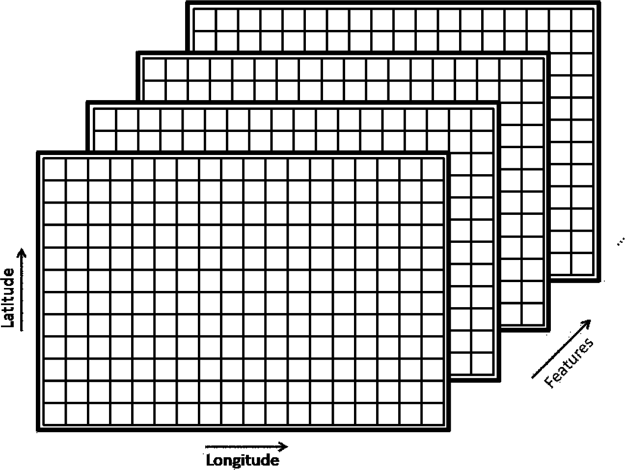
Triclustering is a computational technique in the data mining field. The entire catalog of techniques and procedures of data mining have a common and general goal: extracting hidden, valid and useful information from large volumes of data. Triclustering is the evolution of a widely-known computational technique, clustering, which involves grouping data based on features’ similarity. Clustering works in a 1D space, while triclustering works in a 3D space.
TriGen [
6] is an algorithm that applies a triclustering technique based on the paradigm of evolutionary algorithms, in particular genetic algorithms [
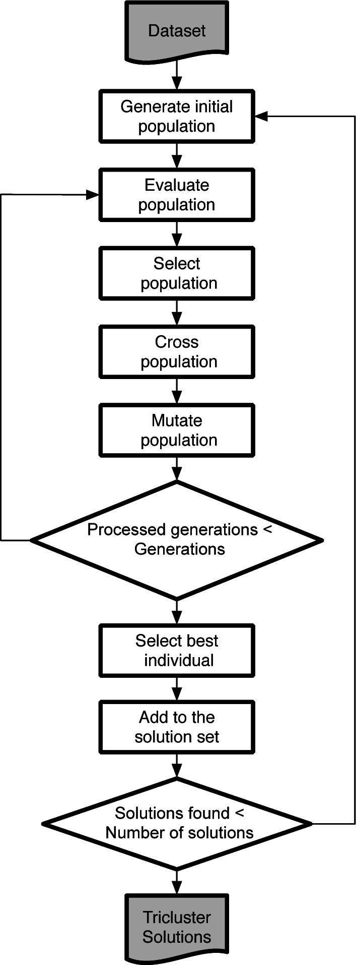
48]. Genetic algorithms perform a heuristic search that mimics the process of natural selection, since a population of individuals is created and evolves throughout several generations using crossover and mutation operators, and the individuals are evaluated based on a function to optimize. For this particular problem, each individual represents a zoning proposal for the IP; the genetic materials of each individual are the longitude and latitude coordinates; and the fitness function maximizes the similarity among all seven features for each cell contained in the zoning. All zones contained in the population are evolved, and after some generations, the optimal one is selected. The flowchart of the algorithm is illustrated in
Figure 3.
TriGen’s steps can be described as: the population initialization step in which the initial population will be created taking into account overlap with previously found solutions; an evaluation step in which each individual will be evaluated using the fitness function; a selection step, which serves to decide which individuals will survive to the next generation; crossover, which creates the necessary connections between pairs of individuals to share new genetic material; and finally, mutation, which performs punctual changes to individuals to ensure genetic variability of future generations.
Each of these operators are now briefly described; for further details please refer to [
6]. The initial population is randomly generated. Part of the individuals are purely randomly generated, that is a random subset of longitudes, latitudes and features are assigned. The rest of the individuals are also randomly generated, but paying attention to overlapping with previously found solutions. This is done to promote the visiting of non-explored areas and the widest area possible of the database.
As for the crossover operator, two individuals (or parents) are combined to create two new individuals (or offspring). They are chosen based on a probability of crossover parameter, denoted by pc. Their genetic materials (latitude and longitude) are randomly combined, mixing the coordinates in both children.
An individual can be mutated according to a probability of mutation, pm. The pm condition is verified for every individual, and if it is satisfied, one out of six possible actions is taken. These actions are: add/remove a new random latitude coordinate or add/remove a new longitude coordinate.
The selection operator was implemented following the roulette wheel selection method [
49].
Another key question is the selection of the fitness function. The fitness of each individual allows the algorithm to determine the best candidates to remain in subsequent generations. For this particular case, the authors in [
6] proposed a measure based on a three-dimensional adaptation of the mean square residue measure (MSR), which is a classical clustering measure for gene expression analysis [
50], referred to as
fmsr. This measure maximizes the coherence in the behavior of the seven features for all of the cells contained in the zoning. Additionally, the same authors proposed an evaluation measure for triclusters called the multi-slope measure, based on the similarity among the angles of the slopes formed by each profile formed by the genes, conditions and times of the tricluster in [
51].
5. Results
This section describes the results achieved by the application of TriGen to the Iberian Peninsula earthquake database. First, the TriGen parameter setup for this particular case is shown. Then, the zones generated by TriGen are introduced. Finally, the results are correlated with the geology for validation.
5.1. Applying TriGen to Discover Seismogenic Zones
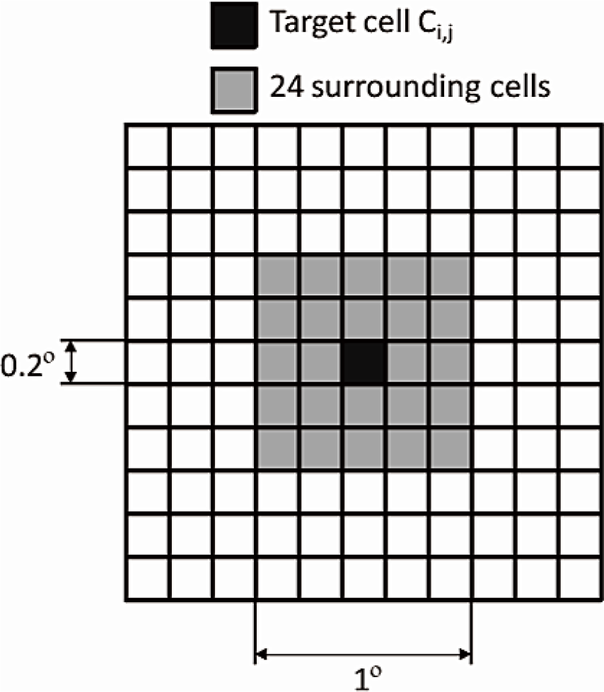
TriGen has been applied to the transformed database described in Section 4.2. By applying this algorithm, we aim to find meaningful patterns for the whole search space, in this case the Iberian Peninsula. In particular, the discovery of zones with similar geophysical properties among the 5400 cells (60×90) is the output of such an algorithm.
Note that TriGen was originally conceived of to deal with temporal data, that is the third dimension being time. In this context, the third dimension is composed of the seven features calculated for every latitude and longitude. In other words, these seven features could be considered seven time stamps for the tuple {
longitude, latitude} introduced in [
6]. Since TriGen is a general-purpose algorithm, it can be applied to any problem formulated on three dimensions. The interpretation of each dimension is up to the context of application.
TriGen can find triclusters, including different numbers of features. However, in this particular research area of the IP with a similar behavior, all seven features under study are intended to be found. Therefore, the algorithm has been forced to generate triclusters including all of the features.
Table 1 shows the selected TriGen setup parameters. The size of the longitude and latitude dimensions are very similar (60 and 90, respectively). Consequently, the same weight for
wlgt and
wltt, 0.4, has been set. The weight for
wf has been set to 1.0, since it is intended that all features appear in all solutions. The overlapping prevention values have been set to 1.0 for longitude,
wdlgt, and latitude,
wdltt, since all of the cells in the IP dataset have to appear in the solution in order to partition the whole space. Nonetheless, the overlapping prevention value for features,
wdf, has been set to 0.0 to allow all features to appear in all solutions.
5.3. Correlation with Geology
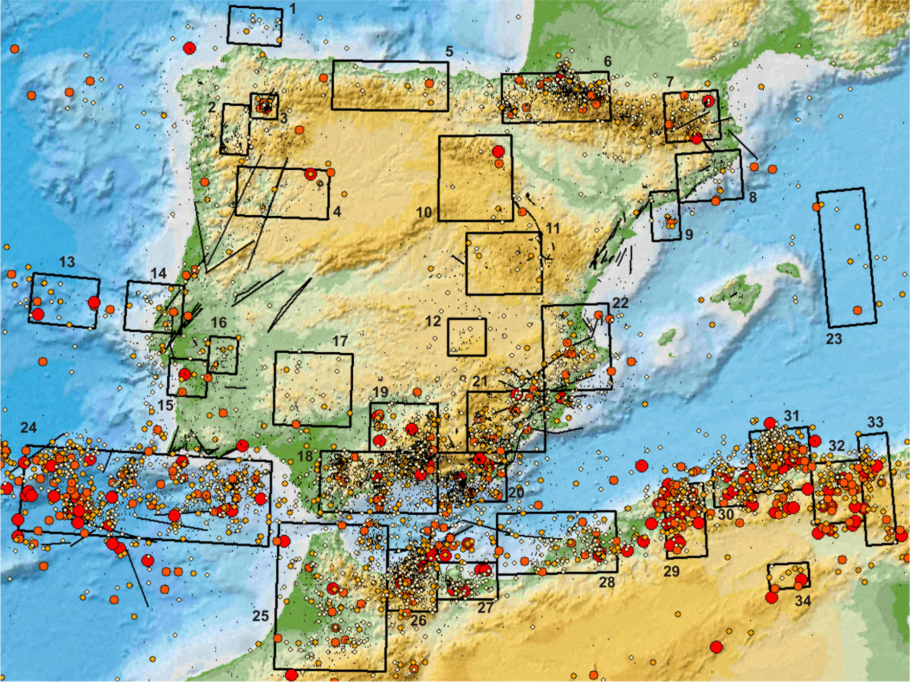
Once the method has been applied and the zones have been obtained, the correlation of the zones with the geology must be verified. In this sense,
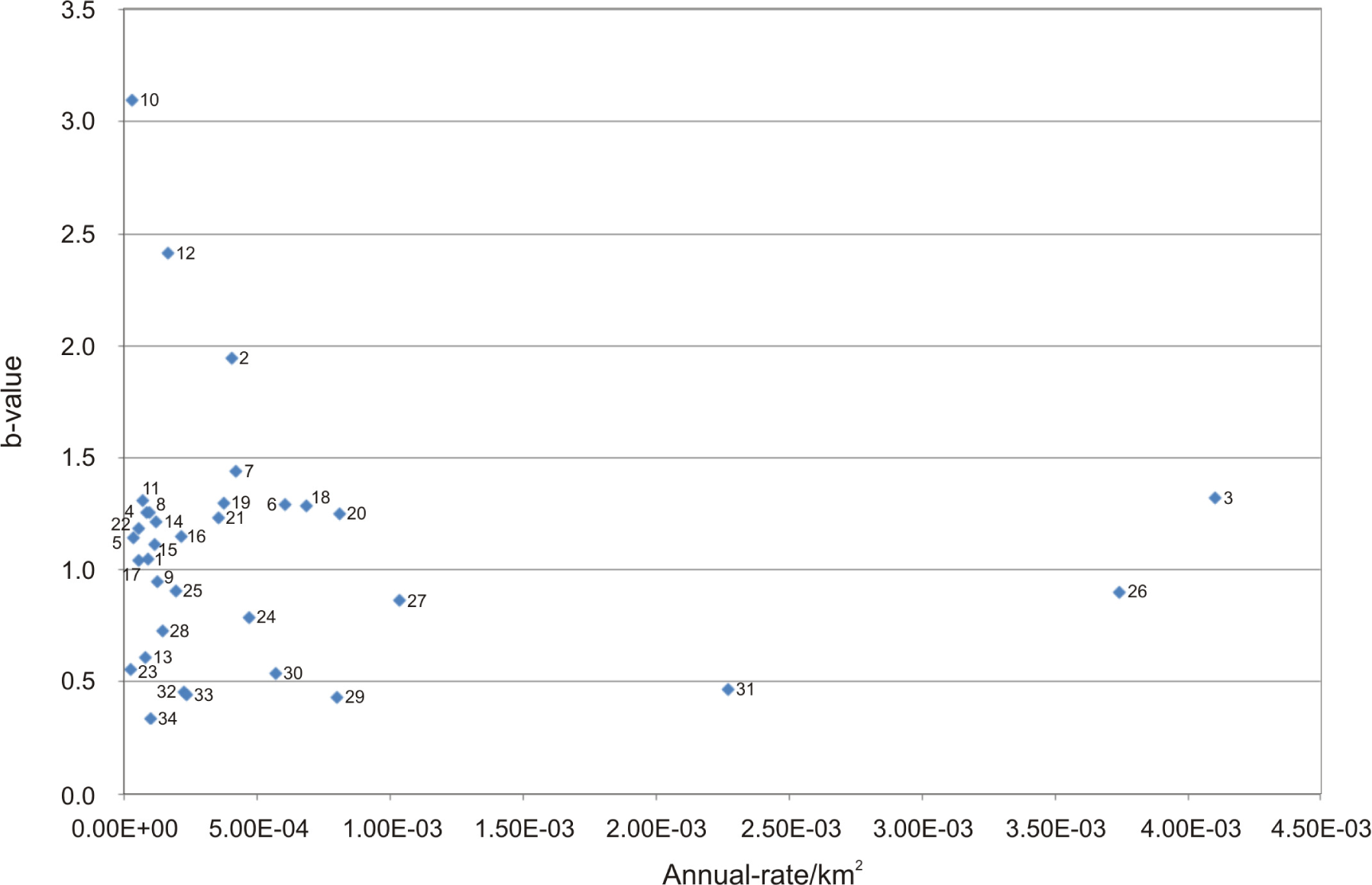
Figure 5 illustrates the annual rate of earthquake occurrence, as well as the associated b-value for every zone discovered by TriGen.
Zone 1 (Z1) is a zone of moderate seismicity and average b-value. It is placed in the north of Galicia. In Z2, the center and south of Galicia, large earthquakes are improbable, and the rate of events is moderate. Contrariwise, in Z3 (east of Galicia), large earthquakes are more probable, and this is the zone with the highest annual rate of earthquakes by km2. Z4 corresponds to Trás-Os-Montes and is a zone of moderate seismicity.
In the Cantabrian Mountains (Z5), earthquakes are infrequent and of moderate magnitude. Z6 and Z7 correspond to the west and the east of the Pyrenees, respectively. They present a similar annual rate of earthquakes and b-value. The Catalan Coastal Range is seismically divided into two: north (Z8) and south (Z9). The southern one has a slightly more frequent annual rate of earthquakes and the lowest b-value.
The Iberian mountain mass is separated into three zones: north (Z10), center (Z11) and south (Z12). The annual rate of earthquakes is moderate, and large earthquakes are improbable. Z13 is a zone located in the west of the coast of Portugal. Large earthquakes are frequent. However, its annual rate is low.
Z14 corresponds to the Mesozoic basins on the west of the Portugal fringe, and it is placed in the west of Z13. Contrarily, large earthquakes are not so frequent. Z15 and Z16 are placed on the Cenozoic basins of the lower Tagus Basin and Tagus Basin, respectively. The b-value is around one, and the annual rate of earthquakes is moderate. Nevertheless, the annual rate of Z16 is twice the rate of Z15.
The Ossa-Morena zone (Z17) presents moderate seismicity. The Betics are divided into four zones (Z18, Z19, Z20 and Z21). It can be observed that the b-value ranges between 1.24 and 1.31. The annual rate of earthquakes is quite high. The zones located in the south (Z18 and Z20) and closer to the contact area between the plates have a higher annual rate of earthquakes.
Z22 is the Valencia Basin and has a moderate seismicity. Z23 is placed on the east of the Balearic Islands. It presents a very low b-value, so the relative number of small and large events is similar. Nonetheless, not many earthquakes hit that zone.
Z24, the Azores-Gibraltar fault, is a very relevant zone, as large earthquakes are known to have occurred within it. Moreover, it is very close to the south of Portugal and the southwest of Spain, and large earthquakes are known to have affected the inland. It is the largest zone depicted and presents a high seismicity rate. Z25 and Z26, the Rif and the east of the Rif, respectively, have the same b-value, but the annual rate of Z26 is much higher. Z27 is located to the east of Z26. It also presents a similar b-value to the two previous ones. It has an outstanding annual rate, but not as high as the east of the Rif zone. To the east, the b-value declines. It is 0.73 for Z28. This zone corresponds to the western part of the Tell.
The b-values of Z29, Z30, Z31, Z32 and Z33 range between 0.44 and 0.54, which points out that large earthquakes are frequent. If the annual rate of earthquakes is examined, it can be observed that it is similar for Z29 (west of the Tell) and Z30 (northwest of the Tell). May be they could be joined into a single zone. The most active zone of this set is Z31 (the north of the Tell), one of the most seismically-hazardous zones examined in this paper. Similarly to Z29 and Z30, the northeast of the Tell (Z32) and the east of the Tell (Z33) have an almost coincident b-value and annual rate, which suggest that they could form a single zone. Finally, Z34, placed at the south of the Tell, has the lowest b-value worked out: 0.34.
6. Comparison to Kohonen’s Self-Organizing Maps
This section is to compare the zoning proposed with the zoning obtained with Kohonen’s self-organizing maps (SOM). SOM [
53] is a special neural network suitable for spatial distribution discrimination. It is trained using unsupervised learning. It generates maps based on a low-dimensional (typically two dimensions) representation of the input space.
The network must be fed with a large number of training vectors that represent the differences exhibited among data during the mapping. In this way, SOM can find the best distribution of zones, based on these training vectors. Since SOM was successfully applied to generate seismic hazard maps in Chile [
46], it has been applied to assess its performance for the Iberian Peninsula. The same input features used for TriGen (see Section 4.3) have been used. Three thousand epochs of 5400 iterations have been used. This number was empirically determined since the use of 1000, 2000, 3000, 5000 and 10,000 epochs did not substantially change the results, and 3000 epochs was advised in [
46].
The number of clusters to be generated is still an open question, and there is no general agreement to determine the optimal number for every case. For this reason, the proposal introduced in [
54] has been applied. This approach combines three well-known indices (silhouette, Davies–Bouldin and Dunn) in a majority vote system. Such indices have been selected due to the different nature of the objectives they maximize. The application of this procedure to the transformed database determined that the best number of partitions is 10.
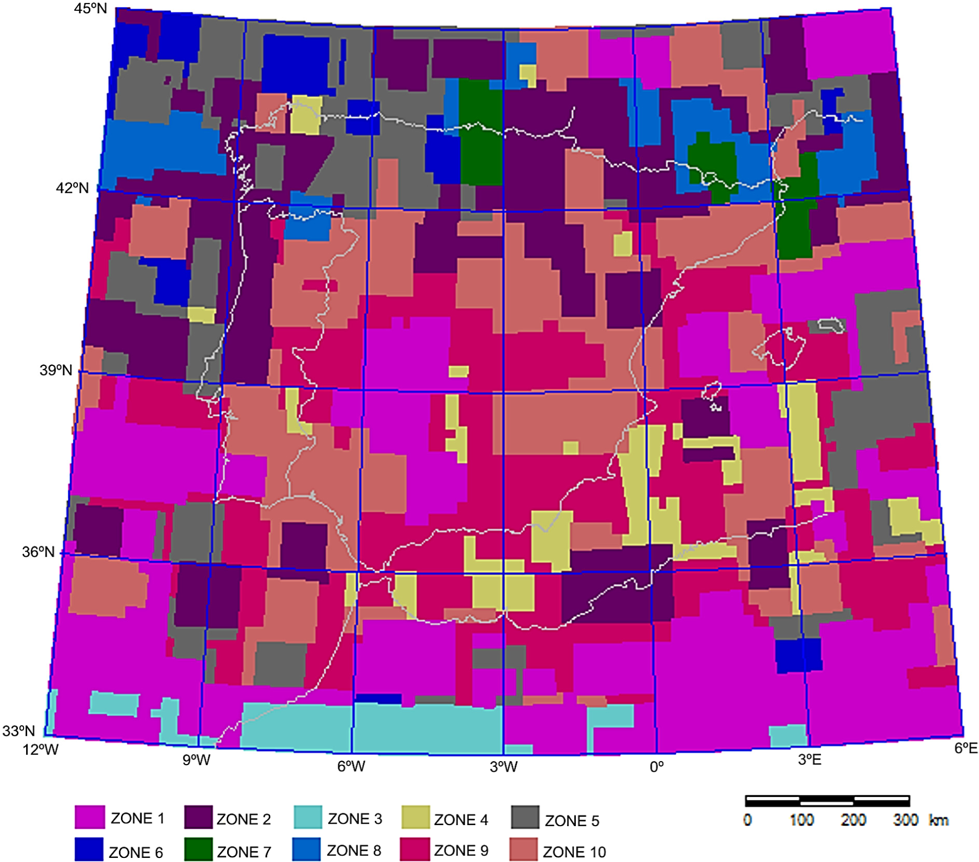
Figure 6 depicts the map obtained when the 7D vectors have been divided into 10 classes. Note that these seven classes did not include the spatial coordinates, longitude and latitude, as input features. Many isolated zones have been labeled similarly. This means that far away zones present similar magnitude histograms. A common procedure in geology is softening the borders of these maps. However, as mentioned before, this procedure is not done in this study.
It can be observed that there is not a continuous structure among the zones found by SOM, and isolated and small zones have been generated with no apparent correlation with the geology. Obviously, these results cannot be considered satisfactory, since they should delimitate particular areas with meaningful information, which is not the case.
To improve the quality of the results, a second scenario has been considered. Similar to [
46], the coordinates of every cell have also been used as input features (see
Figure 7). This new scenario provided a more compact zoning.
If the map shown in
Figure 7 is examined in detail, some vague correlations with geology can be made. Zones 1 and 6 in the south of the IP correspond to the Azores-Gibraltar fault and the north of the Africans plate. Zones 1 and 7 in the center of the IP show the low seismic activity zones of the Central Massif and the Mesozoic basins. It can be observed that Zone 5 coincides with the Alboran Sea, the southeast of the IP and the south of the Balearic Islands. The Pyrenees present a very complex structure represented by labels 2, 9 and 10, similarly to the zoning in [
43]. The Azores-Gibraltar fault, Z24 in this study, has been characterized by labels 1, 5 and 8. Seismicity in Portugal was mainly labeled 7 and 8.
It can be observed that the results provided by the SOM are not as satisfactory as expected. In [
46], the authors properly zoned the whole of continental Chile into just six zones. The coordinates for every cell have been used as inputs, and the division was done considering cells of 1°×1°. In this study, 34 zones have been considered for the IP, and the size of the cells is 0.2°×0.2°.
This could mean that SOM is only valid for zoning high seismic activity areas, such as Chile, into a small number of zones. However, for zoning the IP, a larger number of zones is required. This is due to the fact that the seismicity of the IP is spread over a wide area of deformation. A larger number of zones is required owing to its complexity and a smaller-sized cell is needed.
7. Critical Discussion
The objective of this section is to provide a critical review of the method. The main features of the method and its application to be IP are discussed.
A key issue on seismic zoning is that every zone must be different from the adjacent ones. In order to obtain accurate results, the b-value must be estimated properly. Therefore, only earthquakes after the year of completeness of the catalog must be used. Furthermore, all of the magnitudes must have been calculated with the same procedure. For that purpose, only earthquakes from 1978 onwards have been used in this study. However, a catalog that gathers the largest possible earthquakes must be of a very long duration, probably of hundreds of years. In this research, the catalog has been limited to the 34-year period between 1978 and 2013. The historical seismicity has not been considered. The previous zoning proposed for the IP, described in Section 2.1, used the historical seismicity. For the authors of this research, it is more important to present a robust method than its application to the IP. This is the first step in this sense.
The method only generates rectangular zones, a restriction associated with the types of solutions that TriGen provides. Further research must be done in this sense. Nevertheless, from the analysis exposed in Section 5.3 and from
Figure 4, it can be concluded that the results are consistent and that areas of different seismicity have been delimited. Moreover, they correspond with different tectonic units or parts of a tectonic unit with different seismic activity.
The main advantage of this method is that the depicting of the zones is done automatically by the algorithm and that almost no human decision is necessary.
8. Conclusions
A novel seismogenic zoning method has been proposed in this work. To accomplish such a task, a computationally-efficient method based on triclustering has been used. It has been applied to the IP in order to observe its performance. One of the main achievements of this work lies in having avoided the subjective interpretation of experts, as usually happens in this context. That is, the new proposed zones share similar histograms and physical properties and, intentionally, have not been smoothed. To assess TriGen’s performance, the well-known self-organizing maps have also been applied to the Iberian Peninsula data for two different scenarios, since they have already been used satisfactorily in other areas. Although the results obtained showed a certain degree of correlation with the underlying geology, they could not be considered as satisfactory as those obtained with TriGen.


 ,
, 


