
An Integrated Index for the Identification of Focal Electroencephalogram Signals Using Discrete Wavelet Transform and Entropy Measures


Abstract
:1. Introduction

2. Methodology
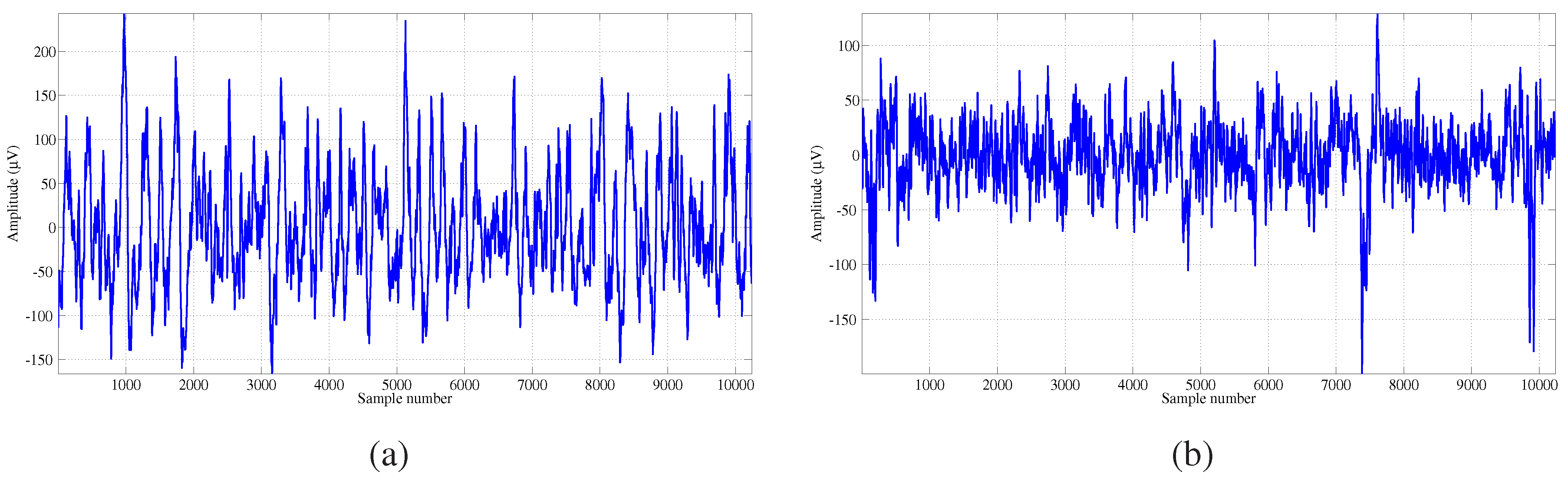
2.1. Dataset


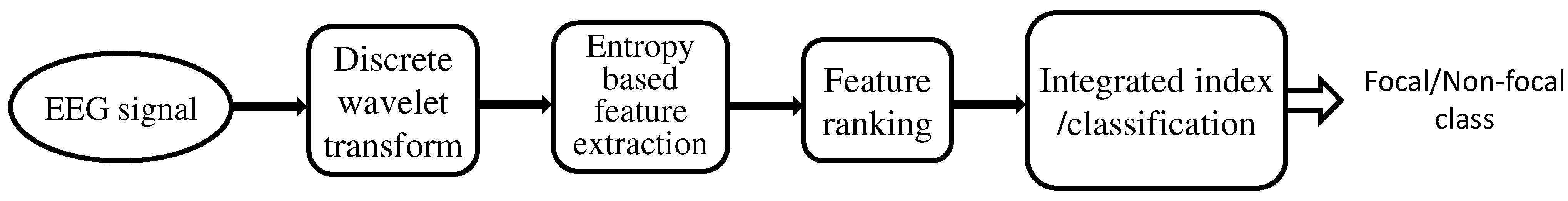
2.2. Feature Extraction
2.2.1. Discrete Wavelet Transform
2.2.2. Average Shannon Wavelet Entropy
2.2.3. Average Rényi Wavelet Entropy
2.2.4. Average Tsallis Wavelet Entropy
2.2.5. Average Fuzzy Entropy
2.2.6. Average Permutation Entropy
2.2.7. Average Phase Entropies
2.3. Feature Ranking
2.3.1. Bhattacharyya Space Algorithm
2.3.2. Student’s t-Test
2.3.3. Wilcoxon Test
2.3.4. Entropy
2.3.5. Receiver Operating Characteristic Method
2.4. Classification
2.4.1. Probabilistic Neural Network
2.4.2. k-Nearest Neighbour
2.4.3. Fuzzy Sugeno Classifier
2.4.4. Least Squares Support Vector Machine
2.5. Integrated Discrimination Index
3. Results

| Feature | Wavelet decomposition level | ||||
|---|---|---|---|---|---|
| 2 | 3 | 4 | 5 | 6 | |
| SwnAvg | 6.000 × 10⁻⁴ | 6.565 × 10⁻⁵ | 9.182 × 10⁻⁷ | 9.511 × 10⁻⁸ | 1.901 × 10⁻⁶ |
| RwnAvg | 2.332 × 10⁻⁶ | 1.336 × 10⁻⁷ | 1.901 × 10⁻⁶ | 6.565 × 10⁻⁵ | 7.000 × 10⁻⁴ |
| TwnAvg | 7.000 × 10⁻⁴ | 8.760 × 10⁻⁵ | 1.495 × 10⁻⁶ | 1.026 × 10⁻⁷ | 2.761 × 10⁻⁶ |
| FzenAvg | 6.722 × 10⁻⁹ | 5.701 × 10⁻⁹ | 4.042 × 10⁻⁷ | 5.766 × 10⁻¹ | 2.495 × 10⁻⁶ |
| Hen1Avg | 4.710 × 10⁻² | 2.890 × 10⁻² | 6.300 × 10⁻³ | 2.510 × 10⁻² | 4.906 × 10⁻¹ |
| Hen2Avg | 2.090 × 10⁻² | 1.770 × 10⁻² | 1.160 × 10⁻² | 2.990 × 10⁻² | 3.379 × 10⁻¹ |
| PzenAvg | 2.690 × 10⁻² | 1.092 × 10⁻⁵ | 5.253 × 10⁻¹⁰ | 5.729 × 10⁻⁶ | 1.638 × 10⁻¹ |


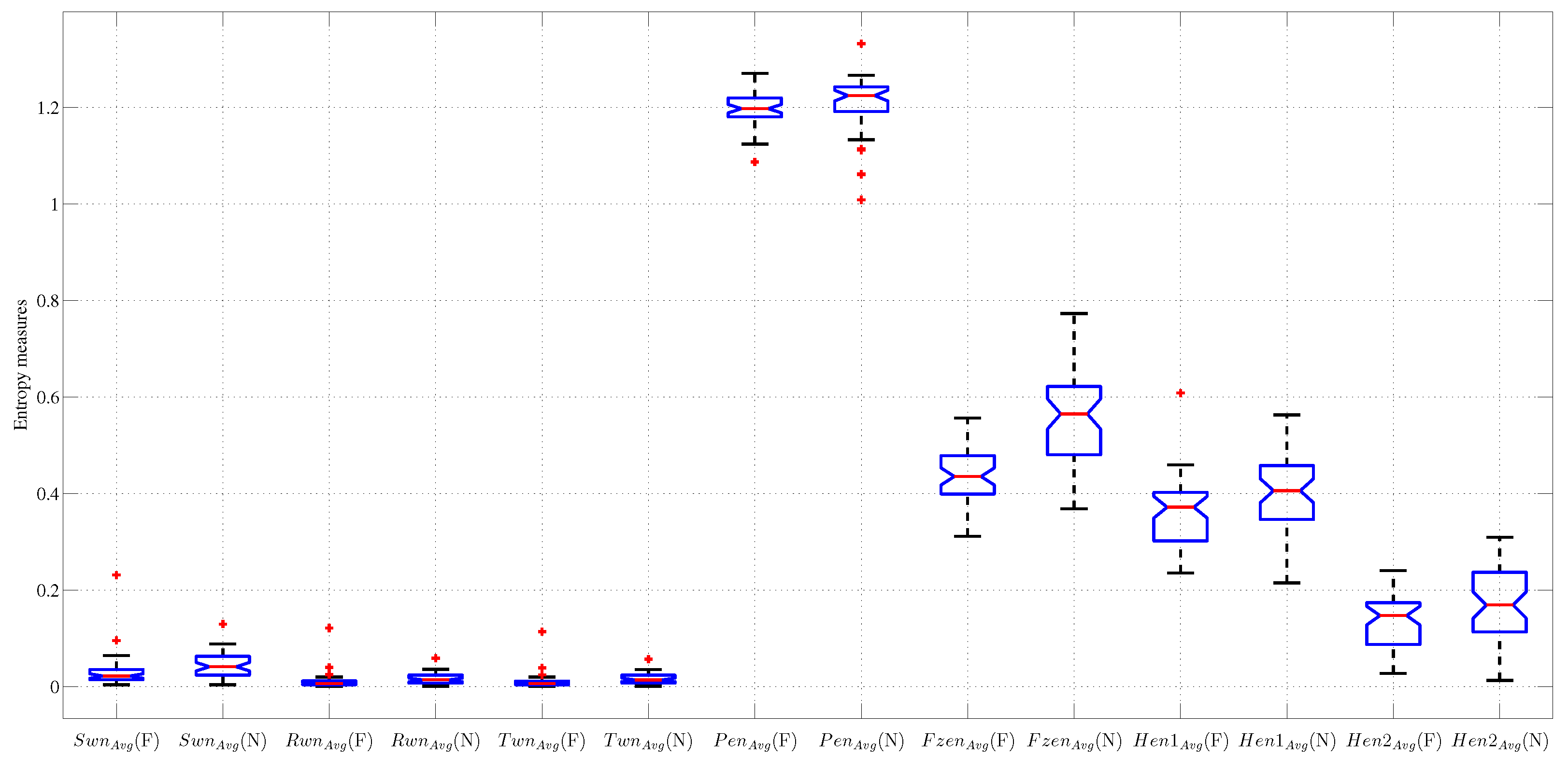
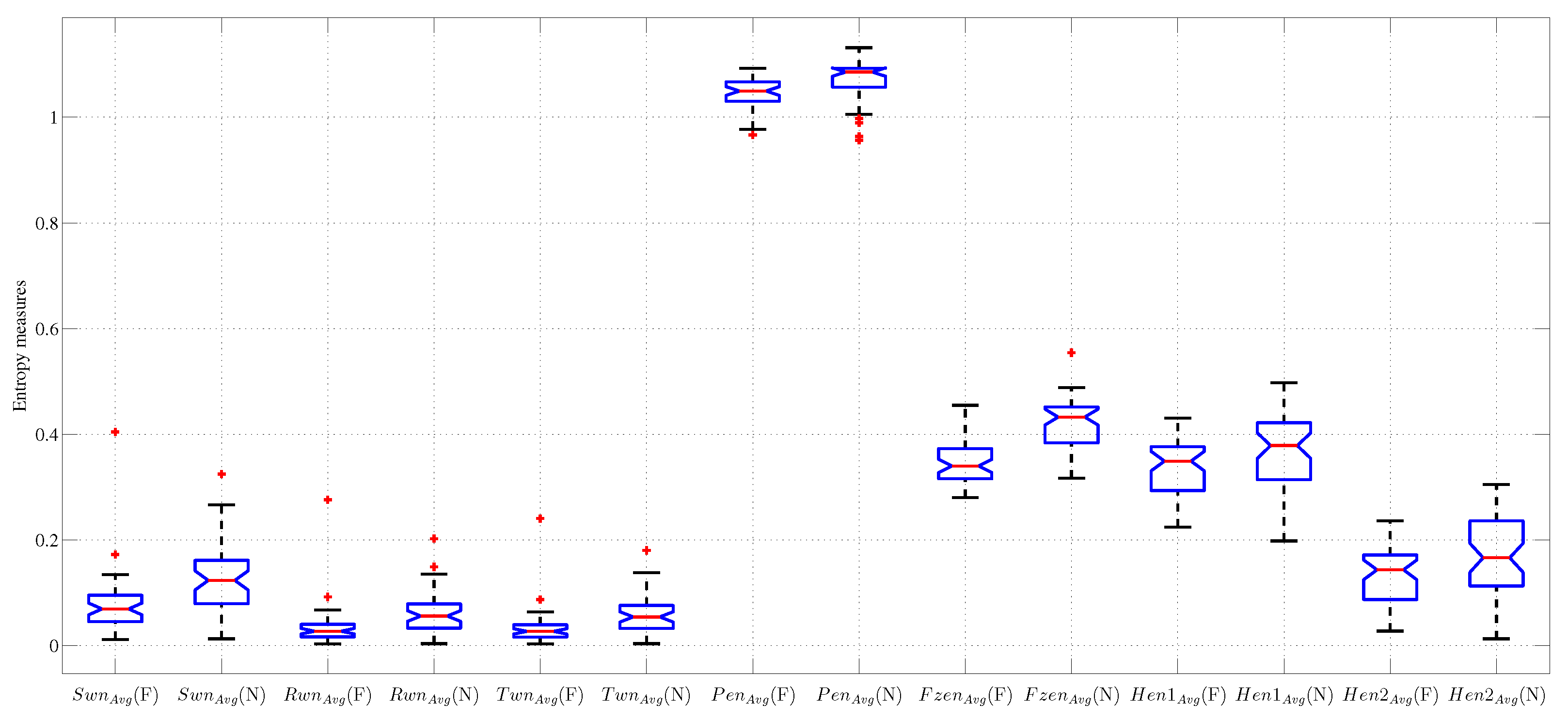
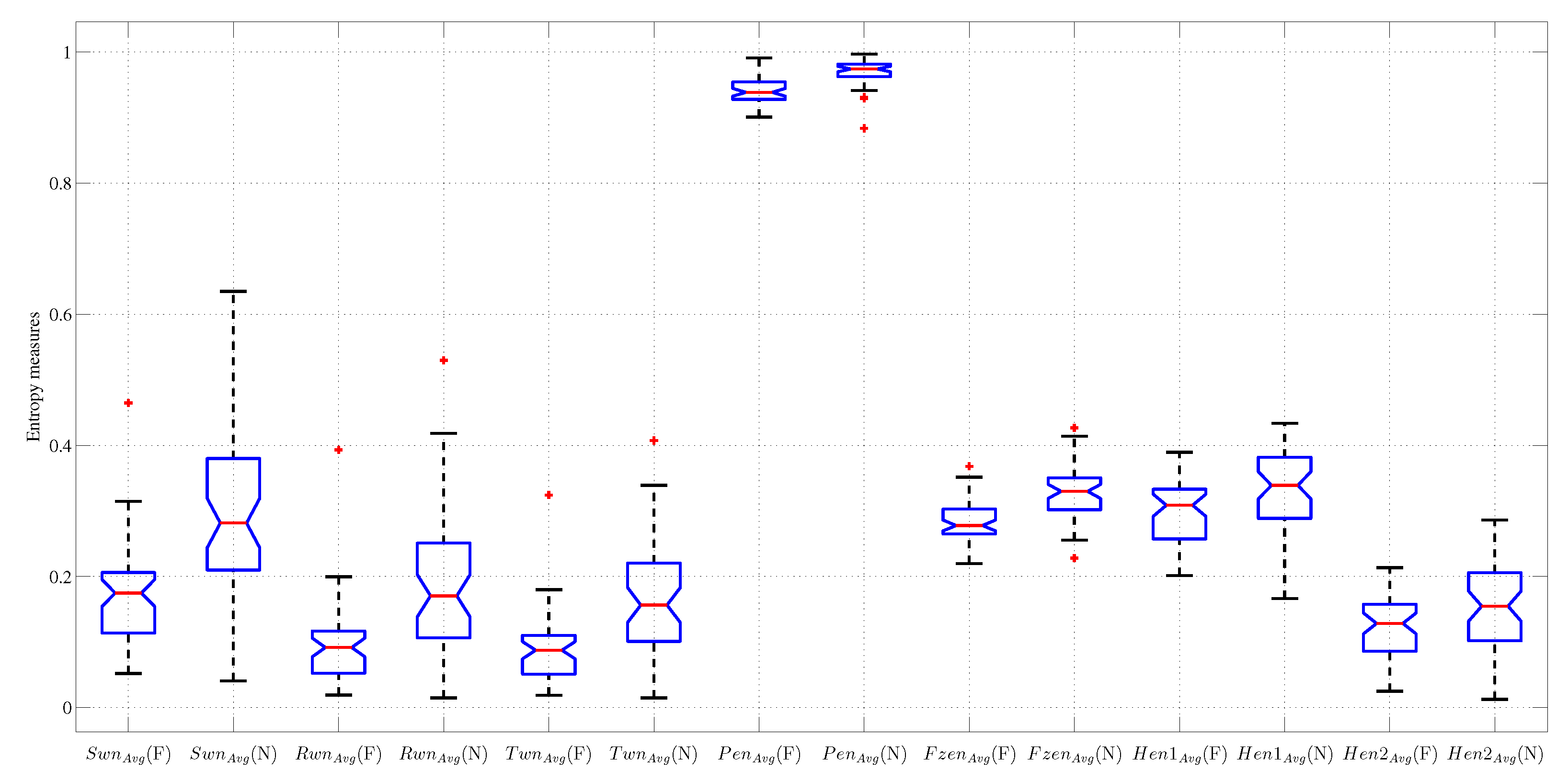
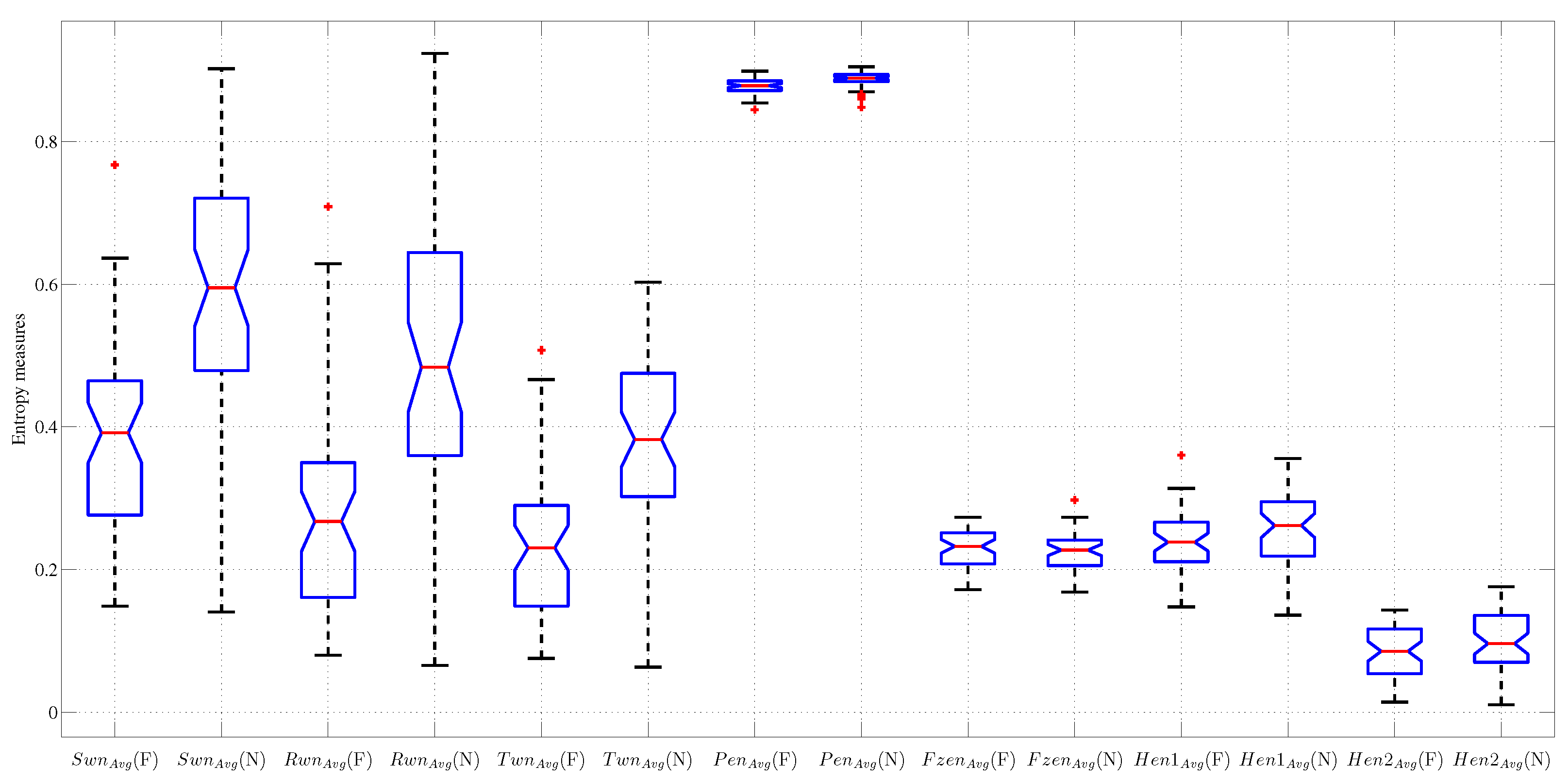
| Feature | Focal EEG signals | Non-focal EEG signals | t-value |
|---|---|---|---|
| SwnAvg | 0.1764 ± 0.0782 | 0.2874 ± 0.1230 | 5.3831 |
| RwnAvg | 0.0970 ± 0.0617 | 0.1810 ± 0.1023 | 4.9688 |
| TwnAvg | 0.0904 ± 0.0521 | 0.1606 ± 0.0813 | 5.1419 |
| FzenAvg | 0.2841 ± 0.0321 | 0.3254 ± 0.0400 | 5.6913 |
| Hen1Avg | 0.3002 ± 0.0470 | 0.3304 ± 0.0628 | 2.7250 |
| Hen2Avg | 0.1212 ± 0.0499 | 0.1536 ± 0.0676 | 2.7228 |
| PenAvg | 0.9414 ± 0.0205 | 0.9698 ± 0.0196 | 7.0752 |

| DWT based decomposition level | Classifier | ROC | Student’s t-test | Bhatacharyya space algorithm | Entropy | Wilcoxon |
|---|---|---|---|---|---|---|
| Second | KNN (k = 1) | 72 | 75 | 75 | 75 | 75 |
| PNN (σ1 = 0.41) | 79 | 81 | 80 | 80 | 80 | |
| Fuzzy (R = 0.1) | 80 | 79 | 81 | 81 | 81 | |
| LS-SVM (σ2 = 3.6) | 77 | 79 | 81 | 82 | 81 | |
| Third | KNN (k = 1) | 75 | 75 | 70 | 70 | 70 |
| PNN (σ1 = 0.21) | 79 | 78 | 79 | 79 | 79 | |
| Fuzzy (R = 0.1) | 81 | 81 | 80 | 81 | 80 | |
| LS-SVM (σ2 = 4.2) | 81 | 80 | 79 | 78 | 80 | |
| Fourth | KNN (k = 1) | 70 | 70 | 74 | 68 | 72 |
| PNN (σ1 = 0.31) | 80 | 80 | 78 | 75 | 76 | |
| Fuzzy (R = 0.1) | 82 | 82 | 81 | 82 | 79 | |
| LS-SVM (σ2 = 4.2) | 84 | 84 | 81 | 83 | 81 | |
| Fifth | KNN (k = 1) | 61 | 61 | 63 | 68 | 68 |
| PNN (σ1 = 0.21) | 75 | 75 | 75 | 75 | 79 | |
| Fuzzy (R = 0.1) | 78 | 78 | 78 | 79 | 81 | |
| LS-SVM (σ2 = 8.6) | 77 | 78 | 77 | 77 | 79 | |
| Sixth | KNN (k = 1) | 70 | 67 | 70 | 67 | 71 |
| PNN (σ1 = 0.21) | 73 | 75 | 73 | 75 | 75 | |
| Fuzzy (R = 0.1) | 78 | 78 | 78 | 76 | 78 | |
| LS-SVM (σ2 = 6.8) | 76 | 77 | 76 | 78 | 77 |
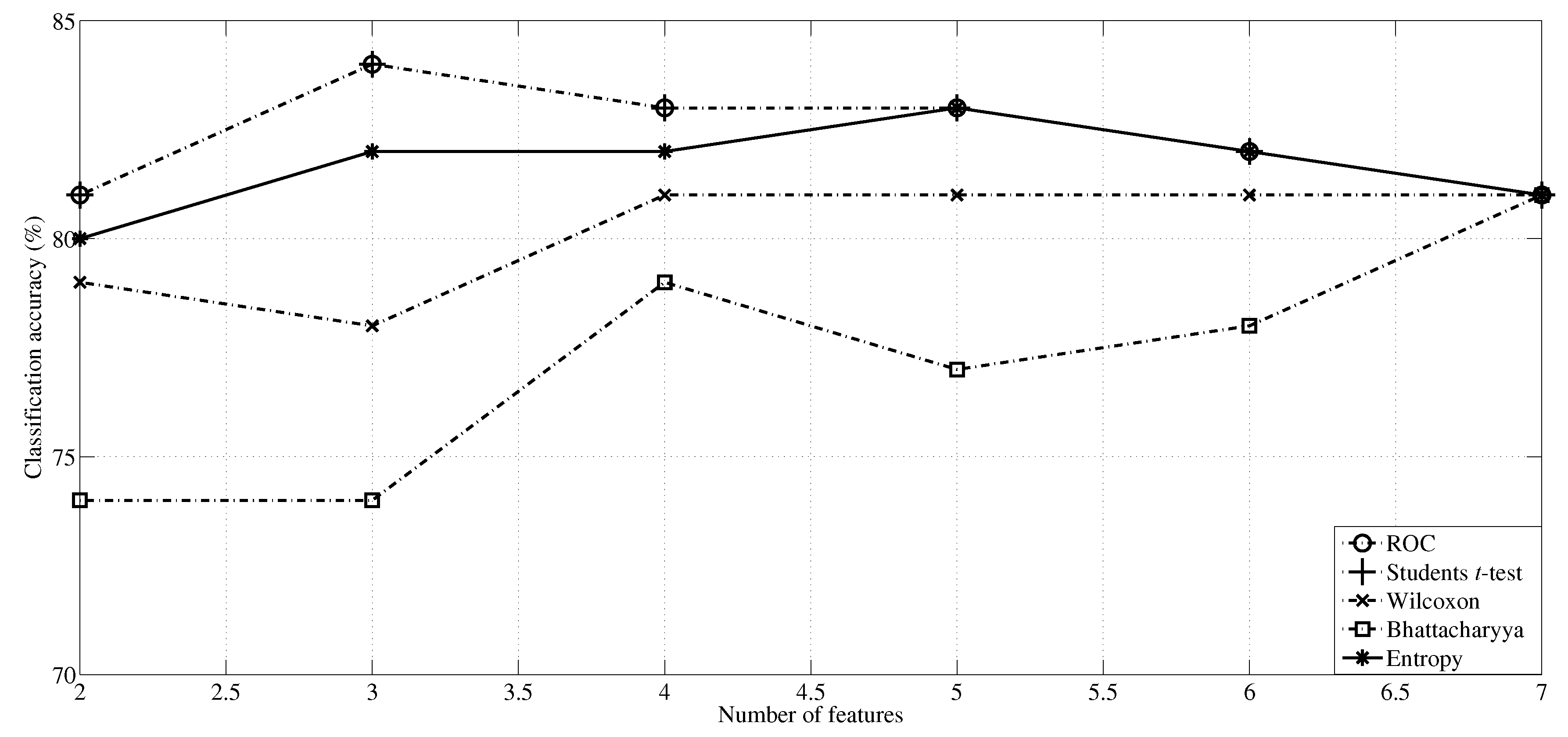
| Ranking method | Number of features | Acc (%) | Sen (%) | Spe (%) |
|---|---|---|---|---|
| Bhattacharyya space algorithm | 7 | 81 ± 8.75 | 78 ± 14.75 | 84 ± 12.65 |
| Student’s t-test | 3 | 84 ± 10.74 | 84 ± 15.77 | 84 ± 12.66 |
| Wilcoxon | 4 | 81 ± 12.86 | 80 ± 21.08 | 82 ± 19.88 |
| ROC | 3 | 84 ± 10.74 | 84 ± 15.77 | 84 ± 12.66 |
| Entropy | 5 | 83 ± 10.59 | 82 ± 14.75 | 84 ± 12.64 |

4. Discussion
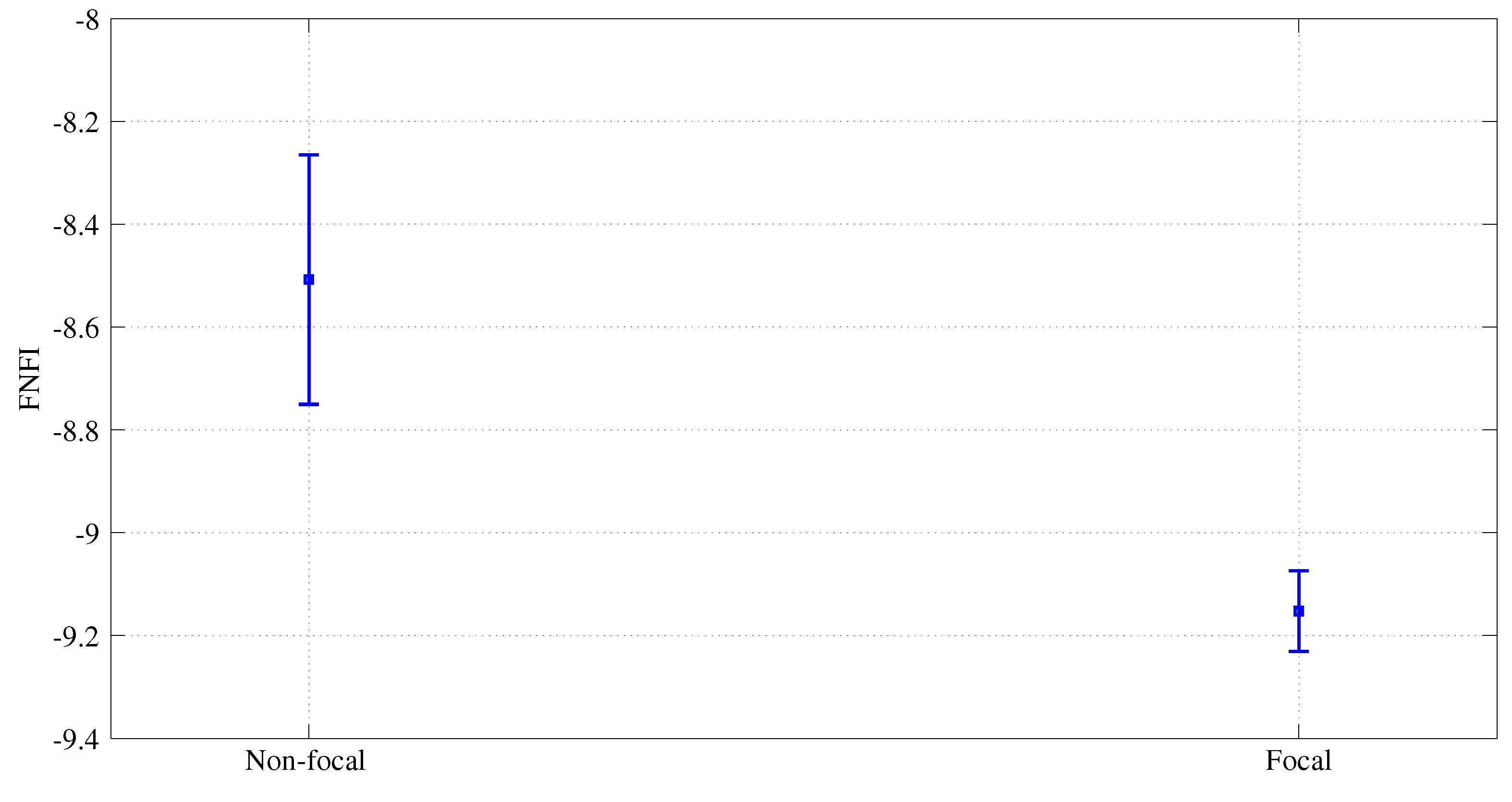
- A novel discrimination index, FNFI, is proposed using three features that can identify focal and non-focal EEG signals using a single number.
- This integrated index can be used by epileptologists to cross-check their diagnosis and, hence, can reduce their workload significantly.
| Authors | Datasets | Features | Classifiers | Ten-fold cross-validation used | Classification accuracy (%) |
|---|---|---|---|---|---|
| Zhu et al. [69] | 50 signals | DPE | SVM | No | 84 |
| 750 signals | 75 | ||||
| Sharma et al. [70] | 50 signals | ASE, AVIF measures from IMFs | LS-SVM | Yes | 85 |
| Sharma et al. [28] | 50 signals | Entropy measures from IMFs | LS-SVM | Yes | 87 |
| This work | 50 signals | Entropy features from DWT | KNN, PNN, fuzzy and LS-SVM | Yes | FNFI clearly discriminates two classes |
5. Conclusion
Author Contributions
Conflict of Interests
References
- Cross, D.J.; Cavazos, J.E. The Role of Sprouting and Plasticity in Epileptogenesis and Behavior; Behavioral Aspects of Epilepsy; Demos Medical Publishing: New York, NY, USA, 2007. [Google Scholar]
- Acharya, U.R.; Sree, S.V.; Swapna, G.; Martis, R.J.; Suri, J.S. Automated EEG analysis of epilepsy: A review. Knowledge-Based Syst. 2013, 45, 147–165. [Google Scholar] [CrossRef]
- Pati, S.; Alexopoulos, A.V. Pharmacoresistant epilepsy: From pathogenesis to current and emerging therapies. Clevel. Clin. J. Med. 2010, 77, 457–467. [Google Scholar] [CrossRef] [PubMed]
- Ortega, G.J.; Menendez de la Prida, L.; Sola, R.G.; Pastor, J. Synchronization clusters of interictal activity in the lateral temporal cortex of epileptic patients: Intraoperative electrocorticographic analysis. Epilepsia 2008, 49, 269–280. [Google Scholar] [CrossRef] [PubMed]
- Van Mierlo, P.; Carrette, E.; Hallez, H.; Raedt, R.; Meurs, A.; Vandenberghe, S.; Van Roost, D.; Boon, P.; Staelens, S.; Vonck, K. Ictal-onset localization through connectivity analysis of intracranial EEG signals in patients with refractory epilepsy. Epilepsia 2013, 54, 1409–1418. [Google Scholar] [CrossRef] [PubMed]
- Towle, V.L.; Carder, R.K.; Khorasani, L.; Lindberg, D. Electrocorticographic coherence patterns. J. Clin. Neurophysiol. 1999, 16, 528–547. [Google Scholar] [CrossRef] [PubMed]
- Schevon, C.A.; Cappell, J.; Emerson, R.; Isler, J.; Grieve, P.; Goodman, R.; Mckhann, G., Jr.; Weiner, H.; Doyle, W.; Kuzniecky, R.; Devinsky, O.; Gilliam, F. Cortical abnormalities in epilepsy revealed by local EEG synchrony. NeuroImage 2007, 35, 140–148. [Google Scholar] [CrossRef] [PubMed]
- Lehnertz, K.; Elger, C. Spatio-temporal dynamics of the primary epileptogenic area in temporal lobe epilepsy characterized by neuronal complexity loss. Electroencephalogr. Clin. Neurophysiol. 1995, 95, 108–117. [Google Scholar] [CrossRef]
- Andrzejak, R.G.; Schindler, K.; Rummel, C. Nonrandomness, nonlinear dependence, and nonstationarity of electroencephalographic recordings from epilepsy patients. Phys. Rev. E 2012, 86, 046206. [Google Scholar] [CrossRef]
- Gajic, D.; Djurovic, Z.; Gligorijevic, J.; Di Gennaro, S.; Savic-Gajic, I. Detection of epileptiform activity in EEG signals based on time-frequency and nonlinear analysis. Front. Comput. Neurosci. 2015, 9. [Google Scholar] [CrossRef] [PubMed]
- Gajic, D.; Djurovic, Z.; Di Gennaro, S.; Gustafsson, F. Classification of EEG signals for detection of epileptic seizures based on wavelets and statistical pattern recognition. Biomed. Eng. Appl. Basis Commun. 2014, 26, 1450021. [Google Scholar] [CrossRef]
- Subasi, A. EEG signal classification using wavelet feature extraction and a mixture of expert model. Expert Syst. Appl. 2007, 32, 1084–1093. [Google Scholar] [CrossRef]
- Kannathal, N.; Choo, M.L.; Acharya, U.R.; Sadasivan, P.K. Entropies for detection of epilepsy in EEG. Comput. Methods Progr. Biomed. 2005, 80, 187–194. [Google Scholar] [CrossRef] [PubMed]
- Acharya, U.R.; Molinari, F.; Sree, S.V.; Chattopadhyay, S.; Ng, K.H.; Suri, J.S. Automated diagnosis of epileptic EEG using entropies. Biomed. Signal Process. Control 2012, 7, 401–408. [Google Scholar] [CrossRef]
- Daubechies, I. Ten Lectures on Wavelets; SIAM: Philadelphia, PA, USA, 1992. [Google Scholar]
- Acharya, U.R.; Vidya, K.S.; Ghista, D.N.; Lim, W.J.E.; Molinari, F.; Sankaranarayanan, M. Computer-aided diagnosis of diabetic subjects by heart rate variability signals using discrete wavelet transform method. Knowledge-Based Syst. 2015, 81, 56–64. [Google Scholar] [CrossRef]
- Rosso, O.A.; Blanco, S.; Yordanova, J.; Kolev, V.; Figliola, A.; Schürmann, M.; Başar, E. Wavelet entropy: A new tool for analysis of short duration brain electrical signals. J. Neurosci. Methods 2001, 105, 65–75. [Google Scholar] [CrossRef]
- Rényi, A. On measures of entropy and information. In Proceedings of the Fourth Berkeley Symposium on Mathematical Statistics and Probability: Contributions to the Theory of Statistics; University of California Press: Berkeley, CA, USA, 1961; Volume 1, pp. 547–561. [Google Scholar]
- Chen, J.; Li, G. Tsallis wavelet entropy and its application in power signal analysis. Entropy 2014, 16, 3009–3025. [Google Scholar] [CrossRef]
- Ramirez-Villegas, J.F.; Ramirez-Moreno, D.F. Wavelet packet energy, Tsallis entropy and statistical parameterization for support vector-based and neural-based classification of mammographic regions. Neurocomputing 2012, 77, 82–100. [Google Scholar] [CrossRef]
- Chen, W.; Wang, Z.; Xie, H.; Yu, W. Characterization of surface EMG signal based on fuzzy entropy. IEEE Trans. Neural Syst. Rehabil. Eng. 2007, 15, 266–272. [Google Scholar] [CrossRef] [PubMed]
- Xie, H.B.; Chen, W.T.; He, W.X.; Liu, H. Complexity analysis of the biomedical signal using fuzzy entropy measurement. Appl. Soft Comput. 2011, 11, 2871–2879. [Google Scholar] [CrossRef]
- Nicolaou, N.; Georgiou, J. Detection of epileptic electroencephalogram based on permutation entropy and support vector machine. Expert Syst. Appl. 2012, 39, 202–209. [Google Scholar] [CrossRef]
- Bandt, C.; Pompe, B. Permutation entropy: A natural complexity measure for time series. Phys. Rev. Lett. 2002, 88, 174102. [Google Scholar] [CrossRef]
- Riedl, M.; Müller, A.; Wessel, N. Practical considerations of permutation entropy. Eur. Phys. J. Spec. Top. 2013, 222, 249–262. [Google Scholar] [CrossRef]
- Acharya, U.R.; Sree, S.V.; Ang, P.C.A.; Yanti, R.; Suri, J.S. Application of non-linear and wavelet based features for the automated identification of epileptic EEG signals. Int. J. Neural Syst. 2012, 22, 1250002. [Google Scholar] [CrossRef] [PubMed]
- Chua, K.C.; Chandran, V.; Acharya, U.R.; Lim, C.M. Analysis of epileptic EEG signals using higher order spectra. J. Med. Eng. Technol. 2009, 33, 42–50. [Google Scholar] [CrossRef] [PubMed]
- Sharma, R.; Pachori, R.B.; Acharya, U.R. Application of entropy measures on intrinsic mode functions for the automated identification of focal electroencephalogram signals. Entropy 2015, 17, 669–691. [Google Scholar] [CrossRef]
- Acharya, U.R.; Ng, E.Y.K.; Eugene, L.W.J.; Noronha, K.P.; Min, L.C.; Nayak, K.P.; Bhandary, S.V. Decision support system for the glaucoma using Gabor transformation. Biomed. Signal Process. Control 2015, 15, 18–26. [Google Scholar] [CrossRef]
- Kailath, T. The divergence and Bhattacharyya distance measures in signal selection. IEEE Trans. Commun. Technol. 1967, 15, 52–60. [Google Scholar] [CrossRef]
- Zhu, W.; Wang, X.; Ma, Y.; Rao, M.; Glimm, J.; Kovach, J.S. Detection of cancer-specific markers amid massive mass spectral data. Proc. Natl. Acad. Sci. USA 2003, 100, 14666–14671. [Google Scholar] [CrossRef] [PubMed]
- Derryberry, D.R.; Schou, S.B.; Conover, W.J. Teaching rank-based tests by emphasizing structural similarities to corresponding parametric tests. J. Stat. Educ. 2010, 18, 1–19. [Google Scholar]
- Kruskal, W.H. Historical notes on the Wilcoxon unpaired two-sample test. J. Am. Stat. Assoc. 1957, 52, 356–360. [Google Scholar] [CrossRef]
- Mann, H.B.; Whitney, D.R. On a test of whether one of two random variables is stochastically larger than the other. Ann. Math. Stat. 1947, 18, 50–60. [Google Scholar] [CrossRef]
- Bergmann, R.; Ludbrook, J.; Spooren, W.P.J.M. Different outcomes of the Wilcoxon-Mann-Whitney test from different statistics packages. Am. Stat. 2000, 54, 72–77. [Google Scholar]
- Theodoridis, S.; Koutroumbas, K. Feature selection. In Pattern Recognition, second ed.; Academic Press: San Diego, CA, USA, 2003; pp. 163–205. [Google Scholar]
- Kohavi, R. A study of cross-validation and bootstrap for accuracy estimation and model selection. In Proceedings of the 14th International Joint Conference on Artificial Intelligence (IJCAI-95), Montreal, QC, Canada, 20–25 August 1995; Morgan Kaufmann: San Francisco, CA, USA, 1995; pp. 1137–1143. [Google Scholar]
- Swapna, G.; Acharya, U.R.; Sree, S.V.; Suri, J.S. Automated detection of diabetes using higher order spectral features extracted from heart rate signals. Intell. Data Anal. 2013, 17, 309–326. [Google Scholar]
- Mao, K.; Tan, K.C.; Ser, W. Probabilistic neural-network structure determination for pattern classification. IEEE Trans. Neural Netw. 2000, 11, 1009–1016. [Google Scholar] [CrossRef] [PubMed]
- Han, J.; Kamber, M.; Pei, J. Classification: Advanced methods. In Data Mining, 3rd ed.; Kamber, J.H., Pei, J., Eds.; The Morgan Kaufmann Series in Data Management Systems; Morgan Kaufmann: Boston, MA, USA, 2012; pp. 393–442. [Google Scholar]
- Ishibuchi, H.; Nakashima, T. Improving the performance of fuzzy classifier systems for pattern classification problems with continuous attributes. IEEE Trans. Ind. Electron. 1999, 46, 1057–1068. [Google Scholar] [CrossRef]
- Acharya, U.R.; Sree, S.V.; Chattopadhyay, S.; Yu, W.; Ang, P.C.A. Application of recurrence quantification analysis for the automated identification of epileptic EEG signals. Int. J. Neural Syst. 2011, 21, 199–211. [Google Scholar] [CrossRef] [PubMed]
- Acharya, U.R.; Sree, S.V.; Ang, P.C.A.; Yanti, R.; Suri, J.S. Application of non-linear and wavelet based features for the automated identification of epileptic EEG signals. Int. J. Neural Syst. 2012, 22, 1250002. [Google Scholar] [CrossRef] [PubMed]
- Vapnik, V.N. The Nature of Statistical Learning Theory; Springer: New York, NY, USA, 2000. [Google Scholar]
- Suykens, J.A.K.; Vandewalle, J. Least squares support vector machine classifiers. Neural Process. Lett. 1999, 9, 293–300. [Google Scholar] [CrossRef]
- Pachori, R.B.; Sharma, R.; Patidar, S. Classification of normal and epileptic seizure EEG signals based on empirical mode decomposition. In Complex System Modelling and Control Through Intelligent Soft Computations; Zhu, Q., Azar, A.T., Eds.; Springer: Switzerland, 2015; Volume 319, pp. 367–388. [Google Scholar]
- Joshi, V.; Pachori, R.B.; Vijesh, A. Classification of ictal and seizure-free EEG signals using fractional linear prediction. Biomed. Signal Process. Control 2014, 9, 1–5. [Google Scholar] [CrossRef]
- Sharma, R.; Pachori, R.B. Classification of epileptic seizures in EEG signals based on phase space representation of intrinsic mode functions. Expert Syst. Appl. 2015, 42, 1106–1117. [Google Scholar] [CrossRef]
- Ghista, D.N. Physiological systems’ numbers in medical diagnosis and hospital cost-effective operation. J. Mech. Med. Biol. 2004, 4, 401–418. [Google Scholar] [CrossRef]
- Acharya, U.R.; Faust, O.; Sree, S.V.; Ghista, D.N.; Dua, S.; Joseph, P.; Ahamed, V.I.T.; Janarthanan, N.; Tamura, T. An integrated diabetic index using heart rate variability signal features for diagnosis of diabetes. Comput. Methods Biomech. Biomed. Eng. 2011, 16, 222–234. [Google Scholar] [CrossRef] [PubMed]
- Acharya, U.R.; Sree, S.V.; Krishnan, M.M.R.; Krishnananda, N.; Ranjan, S.; Umesh, P.; Suri, J.S. Automated classification of patients with coronary artery disease using grayscale features from left ventricle echocardiographic images. Comput. Methods Programs Biomed. 2013, 112, 624–632. [Google Scholar] [CrossRef] [PubMed]
- Acharya, U.R.; Faust, O.; Sree, S.V.; Molinari, F.; Garberoglio, R.; Suri, J.S. Cost-effective and non-invasive automated benign & malignant thyroid lesion classification in 3D contrast-enhanced ultrasound using combination of wavelets and textures: A class of ThyroScanTM algorithms. Technol. Cancer Res. Treat. 2011, 10, 371–380. [Google Scholar] [PubMed]
- Patidar, S.; Pachori, R.B.; Acharya, U.R. Automated diagnosis of coronary artery disease using tunable-Q wavelet transform applied on heart rate signals. Knowledge-Based Syst. 2015, 82, 1–10. [Google Scholar] [CrossRef]
- Acharya, U.R.; Ng, E.Y.K.; Tan, J.H.; Sree, S.V.; Ng, K.H. An integrated index for the identification of diabetic retinopathy stages using texture parameters. J. Med. Syst. 2012, 36, 2011–2020. [Google Scholar] [CrossRef] [PubMed]
- Ocak, H. Optimal classification of epileptic seizures in EEG using wavelet analysis and genetic algorithm. Signal Process. 2008, 88, 1858–1867. [Google Scholar] [CrossRef]
- Yuen, S.Y.; Chow, C.K. A genetic algorithm that adaptively mutates and never revisits. IEEE Trans. Evol. Comput. 2009, 13, 454–472. [Google Scholar] [CrossRef]
- McKight, P.E.; Najab, J. Kruskal-Wallis Test. Corsini Encycl. Psychol. 2010. [Google Scholar]
- Pachori, R.B. Discrimination between ictal and seizure-free EEG signals using empirical mode decomposition. Res. Lett. Signal Process. 2008, 2008, 293056. [Google Scholar] [CrossRef]
- Pachori, R.B.; Bajaj, V. Analysis of normal and epileptic seizure EEG signals using empirical mode decomposition. Comput. Methods Programs Biomed. 2011, 104, 373–381. [Google Scholar] [CrossRef] [PubMed]
- Shah, M.; Saurav, S.; Sharma, R.; Pachori, R.B. Analysis of epileptic seizure EEG signals using reconstructed phase space of intrinsic mode functions. In Proceedings of 9th International Conference on Industrial and Information Systems, Gwalior, India, 15–17 December 2014; pp. 1–6.
- Pachori, R.B.; Avinash, P.; Shashank, K.; Sharma, R.; Acharya, U.R. Application of empirical mode decomposition for analysis of normal and diabetic RR-interval signals. Expert Syst. Appl. 2015, 42, 4567–4581. [Google Scholar] [CrossRef]
- Azar, A.T.; El-Said, S.A. Performance analysis of support vector machines classifiers in breast cancer mammography recognition. Neural Comput. Appl. 2014, 24, 1163–1177. [Google Scholar] [CrossRef]
- Naro, D.; Rummel, C.; Schindler, K.; Andrzejak, R.G. Detecting determinism with improved sensitivity in time series: Rank-based nonlinear predictability score. Phys. Rev. E 2014, 90, 032913. [Google Scholar] [CrossRef]
- Subramaniyam, N.P.; Hyttinen, J. Dynamics of intracranial electroencephalographic recordings from epilepsy patients using univariate and bivariate recurrence networks. Phys. Rev. E 2015, 91, 022927. [Google Scholar] [CrossRef]
- Ben-Jacob, E.; Doron, I.; Gazit, T.; Rephaeli, E.; Sagher, O.; Towle, V.L. Mapping and assessment of epileptogenic foci using frequency-entropy templates. Phys. Rev. E 2007, 76, 051903. [Google Scholar] [CrossRef]
- Marciani, M.G.; Stefanini, F.; Stefani, N.; Maschio, M.C.E.; Gigli, G.L.; Roncacci, S.; Caltagirone, C.; Bernardi, G. Lateralization of the epileptogenic focus by computerized EEG study and neuropsychological evaluation. Int. J. Neurosci. 1992, 66, 53–60. [Google Scholar] [CrossRef] [PubMed]
- Sabesan, S.; Good, L.B.; Tsakalis, K.S.; Spanias, A.; Treiman, D.M.; Iasemidis, L.D. Information flow and application to epileptogenic focus localization from intracranial EEG. IEEE Trans. Neural Syst. Rehabil. Eng. 2009, 17, 244–253. [Google Scholar] [CrossRef] [PubMed]
- Warren, C.P.; Hu, S.; Stead, M.; Brinkmann, B.H.; Bower, M.R.; Worrell, G.A. Synchrony in normal and focal epileptic brain: The seizure onset zone is functionally disconnected. J. Neurophysiol. 2010, 104, 3530–3539. [Google Scholar] [CrossRef] [PubMed]
- Zhu, G.; Li, Y.; Wen, P.P.; Wang, S.; Xi, M. Epileptogenic focus detection in intracranial EEG based on delay permutation entropy. In Proceeding of 2013 International Symposium on Computational Models for Life Science, Sydney, Australia, 27–29 November 2013; Volume 1559, pp. 31–36.
- Sharma, R.; Pachori, R.B.; Gautam, S. Empirical mode decomposition based classification of focal and non-focal EEG signals. In Proceedings of 2014 International Conference on Medical Biometrics, Shenzhen, China, 30 May–1 June 2014; pp. 135–140.
© 2015 by the authors; licensee MDPI, Basel, Switzerland. This article is an open access article distributed under the terms and conditions of the Creative Commons Attribution license (http://creativecommons.org/licenses/by/4.0/).
Share and Cite
Sharma, R.; Pachori, R.B.; Acharya, U.R. An Integrated Index for the Identification of Focal Electroencephalogram Signals Using Discrete Wavelet Transform and Entropy Measures. Entropy 2015, 17, 5218-5240. https://0-doi-org.brum.beds.ac.uk/10.3390/e17085218
Sharma R, Pachori RB, Acharya UR. An Integrated Index for the Identification of Focal Electroencephalogram Signals Using Discrete Wavelet Transform and Entropy Measures. Entropy. 2015; 17(8):5218-5240. https://0-doi-org.brum.beds.ac.uk/10.3390/e17085218
Chicago/Turabian StyleSharma, Rajeev, Ram Bilas Pachori, and U. Rajendra Acharya. 2015. "An Integrated Index for the Identification of Focal Electroencephalogram Signals Using Discrete Wavelet Transform and Entropy Measures" Entropy 17, no. 8: 5218-5240. https://0-doi-org.brum.beds.ac.uk/10.3390/e17085218