1. Introduction
The field of planning has received enormous attention over the last few decades. The development of methods for domain-independent planning help to find better solutions to many real-life and abstract problems [
1]. It is hardly possible to name all possible applications for this class of methods; therefore, research in this area is definitely justified.
The performance of different planning methods is always dependent on the problem size. In general, solving a planning problem for a complex problem is considered a time-consuming task. This fact causes serious limitations in the applicability of these methods in certain classes of problems.
The class of problems considered in this paper assumes a group of entities coexisting in a common environment. The aim is to continuously plan behaviors for all entities in order to reach the highest possible performance of their operation. The group of entities is not homogeneous in terms of observability and management capabilities. Some entities may follow given orders precisely; some may merely provide information about their planned actions. The behavior of the entities is highly dynamic: changes in the observed state occur quickly, which means that there is not enough time to execute a complex planning algorithm between observing the change and having to provide control.
The considered class of problems is defined in an abstract way. The particular problem definition requires providing information about the space in which the entities exist, about the possible behavior of entities, the method of system control, the performance evaluation function,
etc. There are many real-life problems that belong to this class. Hardware entities, like mobile robots or cars [
2,
3], require a method for motion coordination, which has to guarantee safety. Virtual entities, like computational tasks executed on modern, heterogeneous HPC (high-performance computing) systems, require very efficient methods for resource assignment.
The main contribution of this paper is an abstract description of the planning problem for autonomous entities and a proposed method for solving it in a discrete search space. A case study is provided together with detailed solution analysis, which proves correctness and efficiency.
The paper presents a brief state-of-the-art in order to properly position the research in the domain of planning and multiple entity control. The following sections provide a formal definition of the problem and possible solutions based on general-purpose planning methods: A-star and wavefront. Then, the description of the proposed, hybrid algorithm is presented. Finally, a case study is discussed, and the directions of further research are drawn.
2. Planning for Multiple Autonomous Beings
The domain of planning is a very broad and important area of research. Well-known solutions to the domain-independent planning problems are based on the notion of a search space, which has to be searched in order to find suitable solutions. The search space can represent a graph of cities and highways (where searching is relatively simple), but also multidimensional continuous spaces representing the locations of several moving mobile robots in time.
Two basic approaches to the problems of planning can be identified: deterministic methods for searching the state space using a particular strategy for finding the optimal plan can be used for simple problems [
1]; for more complex problems, heuristics-based methods can be applied.
Although domain-independent planning had been researched since the 1980s [
4], it is still being actively researched [
5]. As heuristic search methods are often used as the basis of state-of-the-art planners [
6], methods for constructing heuristic functions are currently one of the most-researched topics in artificial intelligence (AI) planning [
7].
The problems considered in this paper can be addressed using both of the aforementioned approaches to planning. However, the complexity and time constraints will typically enforce the use of heuristics-based approaches.
Dynamic changes in the problem configuration can be addressed with approaches known as planning under uncertainty. These methods assume that a planning entity does not possess full knowledge required to calculate an optimal plan or that the knowledge is partially incorrect. The solutions to these problems have to deal with the problem of uncertainty modeling. In [
8], the methods for modeling uncertainty have been categorized into four groups: conceptual models, analytical models, AI-based models and simulation models. The solutions to these problems are based on probabilistic reasoning, predicting possible situations using probability distributions.
Methods for managing entity groups are also receiving attention in contemporary research. Many different management methods have been applied to specific problems concerning mobile robots management. Some examples of the considered problems are formation control [
9] and cooperative search [
10]. To overcome the problem of real-time requirements, the solutions tend to simplify the planning algorithm or even replace it with behavioral controllers.
For very complex search spaces with dynamic changes of states and goals, good results can be achieved by the use of agent-based approaches. In [
2], software agents were used to solve the dynamic task allocation problem for robots. Simple behaviors of autonomous agents made it possible to generate high-quality solutions for this complex planning problem.
Different planning techniques are suited to different problems. However, most of the existing solutions are not suitable for the class of problems considered in this paper. A very short response time, planning problem complexity and high-quality planning results cannot be achieved by using these state-of-the-art approaches.
3. Definition of the Planning Problem
We assume that a problem in the considered class is composed of a varying number of relatively similar sub-problems, which share the same environment and, therefore, need a common planning method. The sub-problems can be perceived as independent entities, each having different individual goals. The entities coexist in the same state space with time. Each entity is in a particular state in every moment of the considered time frame. The individual goals of each entity can be represented as a desired state or a list of states that have to be achieved.
The environment and the entities determine specific rules of changing the state over time. The rules can be perceived as the abilities of particular entities; therefore, they can differ between individual entities.
The state space defines a notion of collision, which can be caused by two entities being in a particular state at the same time. The collision does not mean that the entities are in the same state. The intuition would rather be that the colliding entities are “too close”, according to a particular metric defined in the space.
Each entity can be manageable or only observable. Manageable entities require planning and follow provided plans. Observable entities provide information about aims or the current individual plan.
Both types of entities can fail to follow the specified plans. Attempts to perform particular transitions between states can fail or result in different transitions with a given probability, which models uncertainty in plan execution.
The solution to the given problem is a set of plans for every manageable entity. Each plan consists of state changes feasible for the particular entity. The set of plans cannot cause any collision and have to handle possible failures in plan execution.
3.1. Formal Model of the Considered Problem
Let S denote a state space. Let us assume the existence of time, and let T denote the time. All dimensions of the search space and the time are discrete, which is the assumption of the algorithm presented in this paper.
Let us assume the existence of a finite set of entities: E. Each entity has an assigned target state (or a set of states) it wants to reach. The aim is to change the state of all entities into the desired target state as quickly as possible. In real-life situations, the state of an individual entity can be composed of multiple attributes, for instance representing the location of an entity (e.g., a robot), its speed and perhaps its battery level. For the purpose of this paper, only the components that are defined in a common domain (e.g., the location, which can be occupied by various entities at different times) will be taken into consideration.
For each entity
e, there is a function defining its activity in the space over time:
It is well-defined for
, where
is now. For
, the function is not yet known. However, for each entity, there is a function defining its feasible activities in the space over time:
which returns a set of possible
functions. The
function represents all limitations of the entity
e, showing which states can be achieved from a given state in a given time.
The coexistence of several entities in the common state space can lead to inadmissible situations, called collisions. A collision occurs in a particular moment of time and involves two entities. It is not defined using the equality of
function values in the same time: two entities may collide being in different states (for example, if they are too close to each other). Therefore, a collision is defined using the following, domain-dependent function:
which returns one when two different entities cannot be in particular states at the same time. Then, we can define a function for detecting inadmissible situations in activity functions:
Using these notions, a feasible plan for a time span
can be defined:
which means that a plan is a set of activity functions, one for each entity, that do not cause collisions.
The uncertainty of the successful execution of specified plans, which was mentioned before, can be modeled using the following exception function:
which returns a set of possible modified activity functions with assigned probability. This function can be used for calculating the collision probability for a feasible plan. One way of solving the given problem would be to accept plans with the collision probability below a certain factor; however, this would result in highly inefficient plans. Different approaches will be presented in the next section.
4. A-Star and Wavefront Algorithms for Multi-Entity Planning
The problem of planning actions for multiple entities coexisting in a common environment, which has been defined in the previous section, can be solved with well-known, general-purpose planning algorithms. However, the algorithms must be adapted to the specific requirements of the problem. This section provides a detailed description of two such algorithms (A-star and wavefront), preceded by the general intuition on the subject of multi-entity planning, as opposed to classical planning for a single entity.
4.1. Important Assumptions
Planning actions for a single entity can be achieved by direct use of general-purpose planning methods. A plan for a set of n entities can be created by simply executing the algorithm n times. Such an approach is simple to implement and efficient to execute; however, the plan created this way is not guaranteed to be feasible. One can imagine various ways of modifying created activity functions, which can lead to feasibility. Unfortunately, it is very hard to ensure the optimality and completeness of such approaches in the general case.
These issues can be overcome by adopting the planning algorithm for the problem of simultaneous planning for all considered entities. This requires redefining the search space and possible transitions between states. In the considered problem, the state
represents the state of an individual entity. For the purpose of planning, these states will be merged into collective states using the activity function
. Each collective state
is a collection of state components for all entities at a given time
t. For
n entities, we have:
Assuming that the original state s was represented by k values (dimensions), each collective state consists of components. Possible collective states encompass all combinations of individual entities’ states, excluding the states for which the collision function evaluatesto one. Such an approach creates a single, collective state space that does not contain any forbidden states. Any plan created in such a space will be feasible. In the following sections, the collective states and the collective state space will be considered.
4.2. The Complexity of Multi-Dimensional Planning
Together with the number of considered entities, the number of state space dimensions increases, while the number of acceptable state transitions slightly decreases, assuming that no two entities can occupy the same location. They both influence the number of state transitions. It needs to be pointed out that suppression of state transition due to reduced acceptable state transitions is much weaker than their growth due to the increasing number of entities, resulting in an increase of dimensions. That is why planning complexity remains proportional to the number of state space dimensions.
Let us use a simple example assuming a two-dimensional state space represented as a square grid with a single entity. There are states, which are locations that the entity occupies, its coordinates being . Let us assume that the entity can move in four ways, thus executing activity functions transiting it according to the von Neumann neighborhood: north, south, east, west. Having two entities on a plane, being a two-dimensional space, yields a four-dimensional state space. A single state is expressed as a quadruple: , while and remain the entities’ locations on the plane. There is an occupation constraint introduced: no two or more entities can occupy the same location on the plane. This reduces the number of transitions in the state space applying: . Assuming that the plane is a grid, , there are states. However, compensating for the occupation constraint, it is actually: .
There have been some efforts carried out regarding state space reduction, e.g., using preferences [
11]. Depending on particular cases, the reduction can be substantial; however, introducing another entity or factor of uncertainty can trigger the growth of the state space beyond the capabilities of the reduction process. There is also ongoing research regarding efficient graph processing solutions that take distributed and parallel processing into consideration [
12].
4.3. Multi-Entity A-Star
The A-star algorithm [
13] is a heuristic search algorithm, which allows one to find the optimal path from a start state to the end state. The path should be understood as a sequence of state changes.
Let us assume a state space, containing a finite set of
n states. As outlined in
Section 4.1, collective states will be used for planning purposes. Therefore, while the basic idea of A-star remains unchanged, the number of states grows significantly, as each consists of a much larger number of dimensions.
In each step of the generated plan, an action must be performed, which means that a state has to be changed into another state, at defined costs.
The state space can be viewed as a directed, weighted graph
G. Put formally, a graph
G is a tuple:
where:
is a set of vertices,
is a set of edges, each indicating a pair of vertices : ,
is a function that assigns a weight to every edge .
This definition (using unique edge identifiers) allows the situation where we have more than one edge between two vertices, which can be important for some planning domains.
The state space representation in a graph
G is as follows:
states are represented by vertices (each state has components),
actions are represented by edges : if an action of changing state from state to state is possible, .
In the case of the considered multi-entity planning problem, each step of the generated plan will represent actions performed by all of the entities in a single time step. Therefore, in this case, we can assume that . This means that all actions performed by all entities in a single time step are equally expensive and that the algorithm will find the sequence of the entities’ moves that will guide them all to the destination states in the shortest possible time. This also means that even when an entity remains in the same state during an action, the cost remains constant: time is passing.
Some dynamic subsets of
S are defined for the purpose of performing the search:
Ƒ denotes the fringe, i.e., the set of vertices, which are the possible candidates for the next move;
V denotes the set of vertices, which have already been visited.
Additionally, we shall define two sequences:
is a sequence of edges, indicating the optimal path from start to goal;
is a sequence of vertices corresponding to .
A sequence of edges is less ambiguous than a sequence of vertices for the cases where two edges and may join the same vertices.
The description of the algorithm is as follows. The problem is defined by selecting the start state, , and the goal state, . The initial state contains the states of all entities at the beginning, and the goal state is composed of the desired location of each entity.
The goal is to find the least expensive path from to , i.e., a sequence of edges for which is the smallest. In practice, the resulting path in fact contains the paths of individual entities to their respective goals.
Each subsequent step is decided upon by selecting the next node () using an evaluation function . The strategy is to choose the state where the sum of the cost of achieving it () and the estimated cost of getting from that node to the goal node (, called the heuristic) is the lowest. Function will be used to record the edge connecting the node to its predecessor in the optimal path.
The algorithm is as follows:
- (1)
Initially assume: , , .
- (2)
Choose the node
to be expanded:
where
is the already known cost of achieving
from
, and
is the value of the heuristic (estimate cost of getting from
to
).
- (3)
If , go to Step 5.
Otherwise, expand node
.
, and do the following:
calculate the value of function g: ,
add to the fringe: .
- (4)
Remove
from the fringe after expansion and move it to the visited set:
- (5)
Reconstruct the optimal path:
- (a)
Let .
- (b)
Let (empty sequences).
- (c)
Append to the beginning of : .
Append to the beginning of : .
- (d)
Let .
- (e)
Let .
- (f)
If , go to Step 5c.
Otherwise, STOP.
For the A-star algorithm to be complete and optimal, the heuristic function
h must be admissible and consistent [
14]. For a heuristic function to be admissible, it must be optimistic,
i.e., it must never overestimate the cost of getting from a certain node to the goal node. For it to be consistent, if the estimated cost of getting to the goal from a certain node
and its successor
(
) is not greater than the sum of the cost of getting from
to
and the estimated cost of getting from
to the goal:
For instance, an intuitively admissible and consistent heuristic for a problem where each entity state is two-dimensional and represents the location of an entity on a planar surface is a multi-dimensional variation of the straight-line distance (SLD) heuristic,
i.e.,
The presented multi-entity A-star algorithm can be used as an efficient method for finding optimal plans for multiple entities coexisting in a common environment. However, the algorithm is not suitable for addressing the problem of plan execution uncertainty. The class of problems considered in this paper includes different levels of entities’ autonomy, predictability and controllability. Therefore, deterministic execution of the calculated, optimal plan cannot be assumed.
One obvious solution to the situation of plan execution error would be to run the planning algorithm once more with the modified initial state of all entities. However, this approach is not possible in the considered problem: the time required for the planning algorithm to finish is too long. To solve the issue of execution unpredictability, a different approach to the planning problem must be involved.
4.4. Multi-Entity Wavefront
The proposed approach to the problem of controlling the entities when they fail to execute a given plan is to prepare alternate solutions in advance. A robust planning algorithm for the considered problem should assume the possibility of execution failure and create a multi-variant plan that covers exceptional situations. The wavefront algorithm can be used to provide such a multi-variant plan.
The wavefront algorithm allows one to find the shortest (least expensive) path in a graph from any starting point to a given goal. There are two steps to the algorithm:
- (1)
vertex labeling;
- (2)
selecting a path.
The labeling provides a guideline to select the shortest path.
Let us assume a search space given by a graph, which is invariant to multi-dimensional or collective issues mentioned earlier:
where
V is a set of vertices,
E is a set of edges, such as
,
is a function that assigns a weight to every edge
and
g is a labeling function:
. There is an initial labeling
. The first step of the algorithm relabels the vertices. The process starts with the goal vertex
g, which is relabeled
. It continues applying breadth-first search to the vertices that have not been labeled with a positive value. At the first step
,
C becomes a set of subsequent vertices to label:
then the labeling is carried out:
where
is a transition cost assigned to the edge corresponding to an activity. The above process is repeated for each element in
C, and it subsequently continues as long as there are any vertices to relabel. This labeling provides a gradient map used in the subsequent step.
The second step of the algorithm, which is selecting a path, begins with an arbitrarily-chosen starting vertex
s and continues according to descending values of function
g at subsequent vertices, being a gradient descent. The path
P is given as an ordered set of vertices:
such as:
where:
One of the most important features of the wavefront algorithm is that it provides a gradient map, which is a result of the vertex labeling process, which allows one to find an optimal path from any state to the goal by simply descending the gradient. This fact allows one to react immediately in any possible situation that can occur in the controlled group of entities.
Traversing the entire state space while labeling might be not feasible: it is too time-consuming or complex. Thus, a hybrid approach is proposed here. The motivation for it is best presented with an example, which is planning for multiple agents, as shown in the next section.
5. A-Star-Wavefront Hybrid Algorithm
Planning for multiple agents is not different from planning for a single agent, except that the number of dimensions in the search space increases. There are also some side effects that need to be taken into consideration. The one considered here regards possible collisions among agents, due to uncertainty. These might happen if the agents are allowed to deviate from the plan; there might also be different reasons for this situation, such as limited controllability, predictability and observability.
A wavefront-based approach seems to be the most suitable for such multi-agent planning with uncertainty, but its time complexity renders it less applicable. On the other hand, the A-star algorithm, having better time complexity, does not provide alternatives in the case that deviations from the plan occur.
The proposed hybrid approach tries to combine the better time complexity of the A-star with the robustness of the wavefront. It assumes that:
there is a global plan provided by the A-star algorithm;
sub-spaces of a possible collision in the search space are identified; they called collision sub-spaces;
for the above sub-spaces, the wavefront algorithm is used to give the optimal path to exit the sub-space, thus to return to the original A-star-based path.
Let us have a plan generated by the A-star algorithm over a state space given as , where . A single vertex represents the location of all involved agents, while an edge represents possible transition to another state, thus an allowed agent move.
There is a possibility of collision detection function
, such as:
where
N is a neighborhood of states, such as
, such that
, and
, being a collision sub-space, is a state sub-space for the wavefront algorithm subdivided from
G in such a way that
. In such a case, the goal for the wavefront is
, being the last state in the neighborhood of states. There can be a set of the sub-spaces
for a given
identified.
As a result, if an agent deviates from the original plan and the deviation occurs in any of the previously-identified areas covered by any S, a wavefront-generated path is used to return to the original plan as quickly as possible.
The function is a heuristic. It should consider domain-specific properties of the agents, which reflects the likelihood of collision. Increasing the cardinality of S requires more calculations, but makes the plan more robust at the same time.
The number of states, or transitions, if there are any unreachable states, is the core factor of computational complexity, no matter what planning algorithm is used. The proposed hybrid approach is a solution that balances complexity with uncertainty. The proportion is kept by the heuristic function
described earlier. There are two factors that influence the computational complexity of the proposed algorithm:
- (1)
the number of neighborhoods (N) that might result in collisions, either among agents or obstacles: ;
- (2)
the size of the collision sub-space (S): .
More neighborhoods make the solution more robust, and this takes more uncertainty into account. With larger collision sub-spaces, more significant deviations can be covered. However, the increase of both the number of neighborhoods and their size makes it necessary to perform more computations to synthesize the plan.
A collision neighborhood can be heuristically defined as a sequence in the plan, for which particular agents get close to each other at a distance smaller than some given . The particular value should take the properties of the world being modeled into consideration; these include the likelihood of slipping, the uncertainty of agents’ behavior, their controllability, observability, autonomy, etc.
The collision sub-space size should take physical aspects of the agents into consideration. These include the maximum and minimum speed and acceleration, mass, etc.
6. Experimental Results
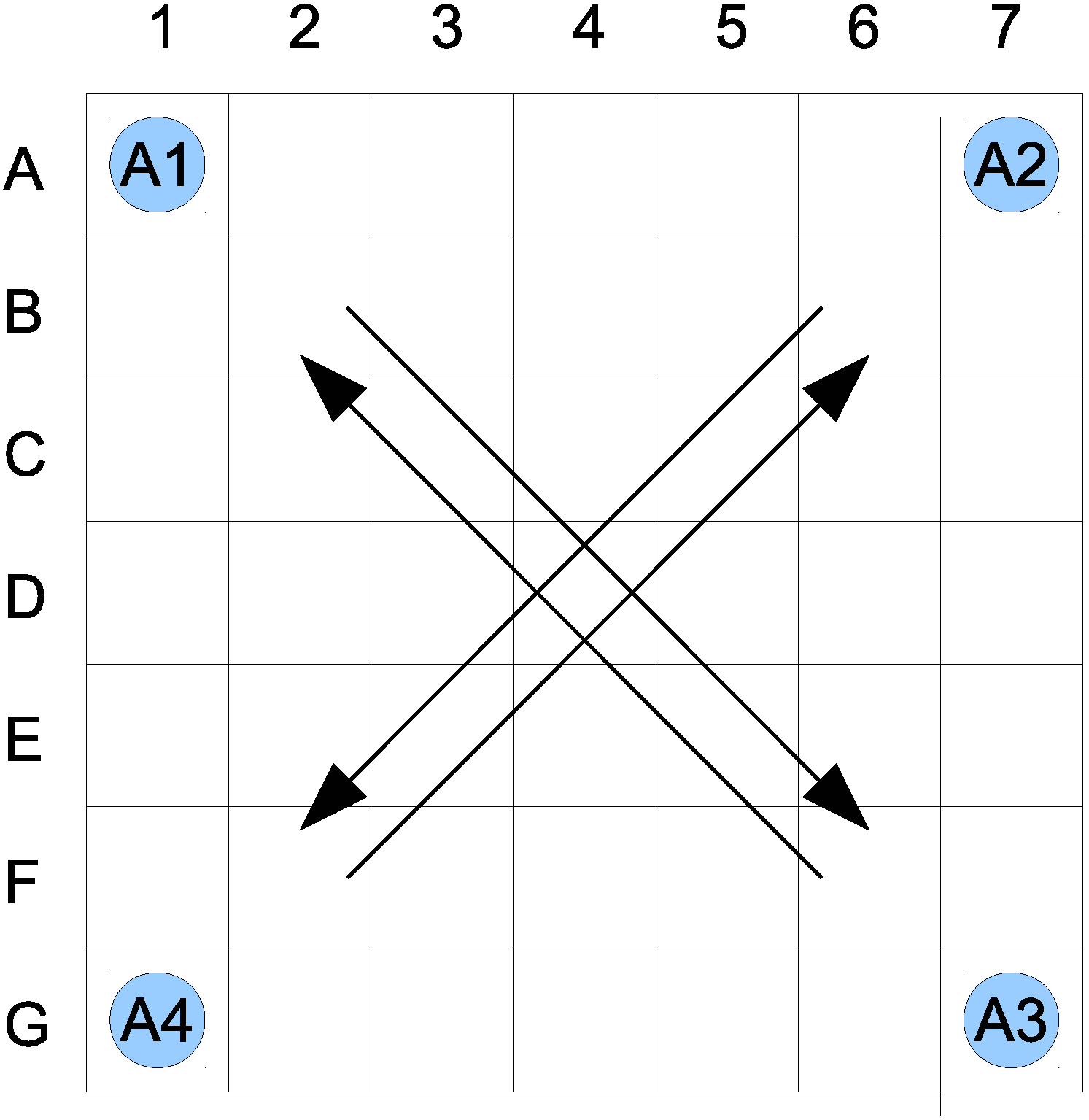
Let us assume that the world being considered is a two-dimensional space, based on a seven by seven grid. The agents, denoted as
, can move from one location to another only orthogonally, in accordance to the von Neumann neighborhood, north, south, east and west, which defines their activity functions. A single location is allowed to be occupied by no more than one agent. There are four agents initially located in the corners (see
Figure 1). Each agent’s goal is to get to the diagonally-opposite corner;
to
,
to
,
to
,
to
. The global goal is to guide all of the agents to their goal corners.
Figure 1.
Initial state of the proposed world.
Figure 1.
Initial state of the proposed world.
Assuming the above, a state consists of the information about agent locations; thus, it is a tuple: , where , , , correspond to locations of agents , , , , respectively.
A good indication of the complexity of A-star-based search complexity is the number of states that have to be considered before the goal is reached,
i.e., the number of heuristic function computations for candidate states. For the given example, assuming a von Neumann neighborhood and a straight-line distance heuristic, the number of these operations is:
The A-star approach does not give robustness and cannot handle uncertainty.
Assuming that each agent can be at any location, having a grid and applying the wavefront algorithm, the computational complexity is proportional to the state space cardinality. It is given as: . Applying the world constraints (no two agents sharing the same location) reduces the number of states slightly, having a product of arithmetic progression: . It renders such a fully-robust plan unfeasible to calculate.
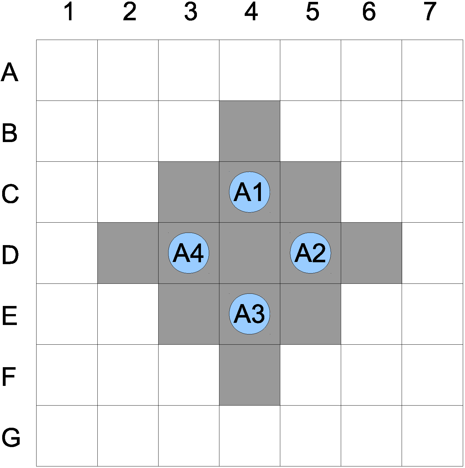
Let us assume a single collision neighborhood with
. This indicates that if an agent comes within a distance of two of any other agent, such a state is identified as a possible collision. The path of the four agents calculated from the A-star algorithm results in a possible collision of all agents at
. Assuming the collision sub-space size
, the actual sub-space is given in
Figure 2. The number of planning operations
is equal to the sub-space cardinality, and it is expressed as:
The total number of operations to establish a robust plan is proportional to:
Figure 2.
Possible collision subspace.
Figure 2.
Possible collision subspace.
Comparing to , this makes the problem over 225-times smaller. As a result, there is a plan in a multidimensional space providing optimal paths for multiple agents. The plan is multi-variant to some degree. While executing it, if there is any deviation from the plan within a previously-identified collision sub-space, there are means to return to the previously-optimal path without any additional calculations. However, this does not imply that in such a case, the plan is still optimal. If a deviation takes place outside of the collision sub-space, there are no means to compensate; thus, proper identification of such and their sizes is crucial.
There have been several experiments conducted, with a variable number of dimensions, regarding different strategies for both collision sub-space identification and its size. The number of dimensions varies from four to eight. The collision sub-spaces are identified based on their distance among entities ranging from one to three. Additionally, such a collision space is grown by a factor of zero to three, to increase the robustness of the plan. Depending on the particular experiment and comparing to the wavefront, the proposed method offers a speedup of up to 225. The plan in such a case is still robust, attaining the ability to recover if deviations happen. Comparing its performance with the A-star results in a speedup of down to 0.24. The above numbers indicate that while the proposed robustness costs computational time, this cost is significantly lower than it would be for the total robustness delivered by the wavefront. This enables the proposed approach to be applicable to real-world cases.
7. Conclusions
Establishing a robust plan for multiple entities might easily lead to combinatorial explosion: it renders the planning process infeasible, especially when time constraints have to be met. The paper proposes a solution to this problem by providing a hybrid planing algorithm, based on a combination of the the A-star and wavefront algorithms. A-star is used to establish a single, optimal plan in a multidimensional space, encompassing the states of all entities. Neighborhoods of states in which a need for robustness is anticipated are identified. At each such neighborhood, a sub-space, called the collision sub-space, is defined. Each such sub-space is covered by the wavefront algorithm to calculate all possible plans to return to the original path provided by A-star. Both the identification of the neighborhoods and the size of the collision sub-space are provided based on heuristics. As a result, a partially-robust plan is established.
The proposed algorithm is verified by an example that involves planning for four independent entities in a two-dimensional world. Computational complexity is reduced by a factor of 225, compared to the fully-robust plan.
Further research is mainly on improving the heuristics used for the identification of collision-prone neighborhoods and the determination of the collision sub-space sizes. Furthermore, work is being done to adapt the algorithm to a quasi-continuous environment.


