
The Intrinsic Cause-Effect Power of Discrete Dynamical Systems—From Elementary Cellular Automata to Adapting Animats

Abstract
:1. Introduction


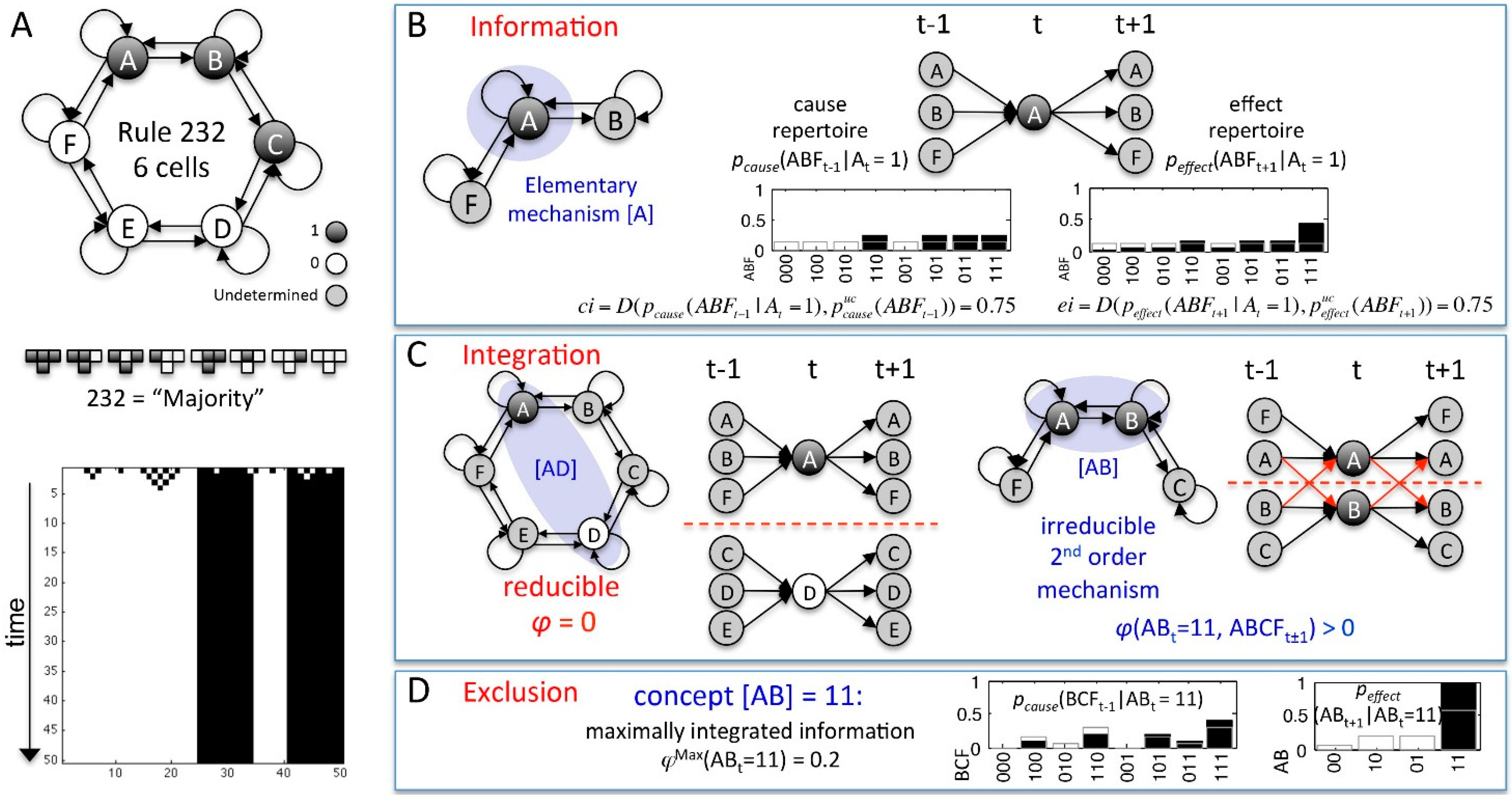
| MECHANISM | cause-effect repertoire | A set of two conditional probability distributions: , describing how the mechanism Mt in its current state mt constrains the past and future states of the sets of system elements Zt-1 and Zt+1, respectively. |
| partition P | , where the connections between the parts and are injected with independent noise. | |
| integrated information φ (“small phi”) | φ measures the irreducibility of a CER w.r.t. a partition P: | |
| MIP | The partition that makes the least difference to a CER: | |
| The set of system elements , where and | ||
| φMax(mt) | The intrinsic cause-effect power of a mechanisms Mt: | |
| concept | The maximally irreducible CER(mt) with φMax(mt) over , describing the causal role of mechanism Mt within the system. | |
| SYSTEM | cause-effect structure C(st) | The set of concepts specified by all mechanisms with φMax(mt) > 0 within the system St in its current state st. |
| ΣφMax | The sum of all φMax(mt) of C(st). | |
| unidirectional partition | , where the connections from the set of elements S1 to S2 are injected with independent noise (for t-1 → t and t → t+1). | |
| integrated conceptual information Φ (“big phi”) | Φ measures the irreducibility of a cause-effect structure w.r.t. a partition : . Φ captures how much the CERs of the system’s mechanisms are altered and how much φMax is lost by partitioning the system. | |
| MIP | The unidirectional system partition that makes the least difference to C(st): | |
| ΦMax | The intrinsic cause-effect power of a system of elements . such that for any other St with , . | |
| complex | A set of elements with . A complex thus specifies a maximally irreducible cause-effect structure. |
2. Results and Discussion
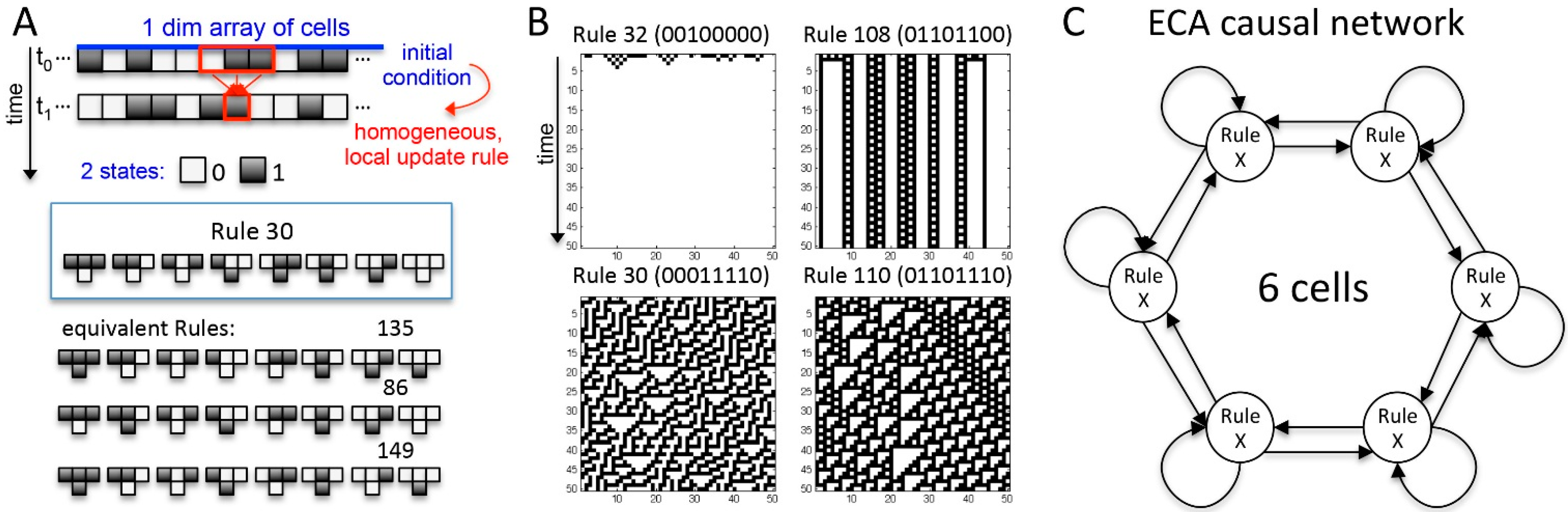
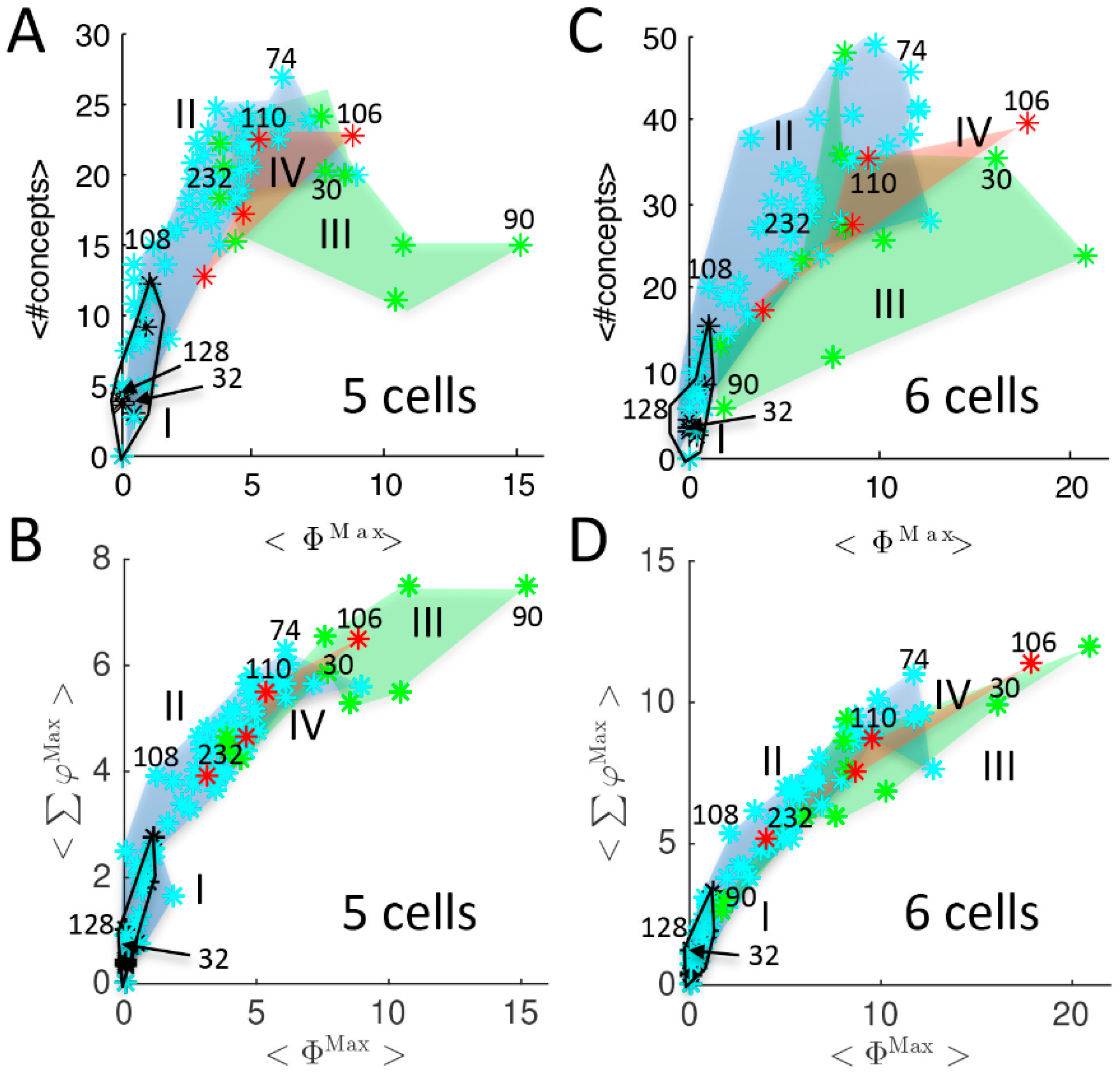
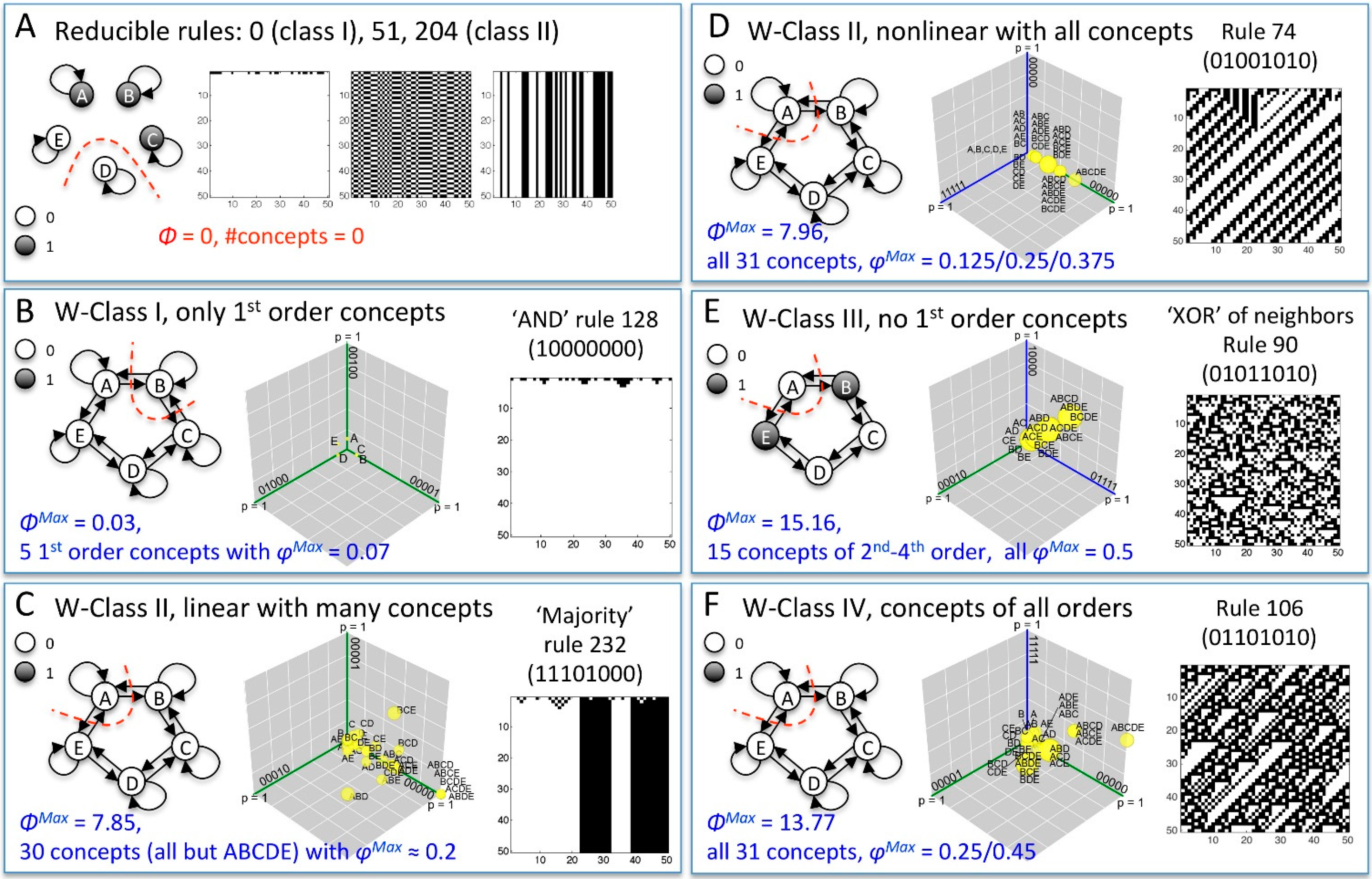
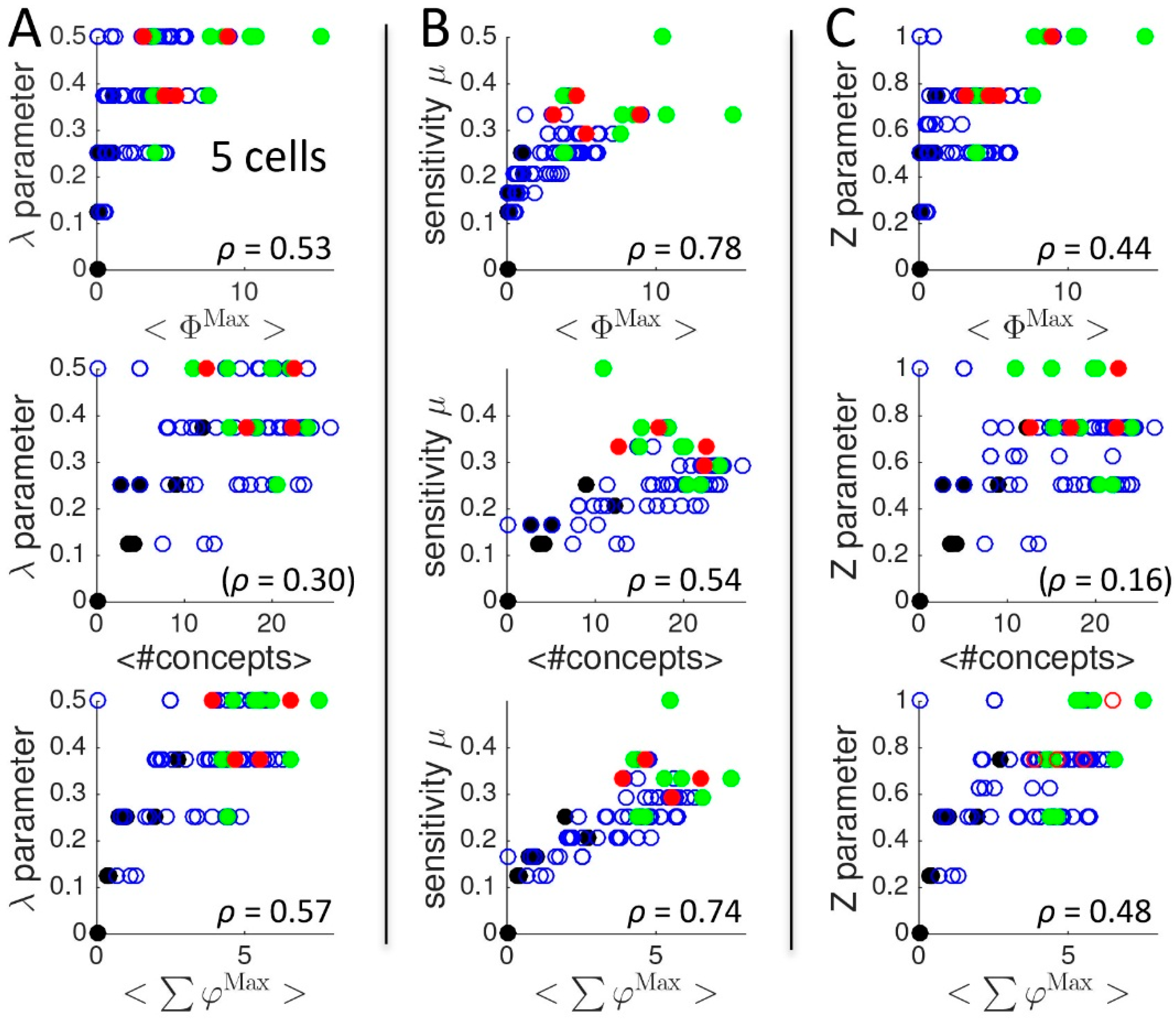
2.1. Behavior and Cause-Effect Power of Elementary Cellular Automata
2.1.1. Cause-Effect Structure of ECA vs. Wolfram Classes


2.1.2. Additional Causal Equivalencies
2.1.3. Comparison to Several Rule-Based Indicators of Dynamical Complexity

2.1.4. Other Types of Classifications
2.1.5. Being vs. Happening


2.2. Behavior and Cause-Effect Power of Adapting Animats

3. Conclusions
4. Methods

4.1. Mechanisms and Concepts
4.2. Cause-Effect Structures

4.3. Transient Lengths
4.4. Statistics and IIT Code
Supplementary Files
Supplementary File 1Supplementary File 2Acknowledgments
Author Contributions
Conflicts of Interest
References
- Nykamp, D. Dynamical System Definition. Available online: http://mathinsight.org/dynamical_system_definition (accessed on 15 May 2015).
- Ermentrout, G.B.; Edelstein-Keshet, L. Cellular automata approaches to biological modeling. J. Theor. Biol. 1993, 160, 97–133. [Google Scholar] [CrossRef] [PubMed]
- De Jong, H. Modeling and simulation of genetic regulatory systems: A literature review. J. Comput. Biol. 2002, 9, 67–103. [Google Scholar] [CrossRef] [PubMed]
- Nowak, M.A. Evolutionary Dynamics; Harvard University Press: Cambridge, MA, USA, 2006. [Google Scholar]
- Sumpter, D.J.T. The principles of collective animal behaviour. Philos. Trans. R. Soc. Lond. B. Biol. Sci. 2006, 361, 5–22. [Google Scholar] [CrossRef] [PubMed]
- Kaneko, K. Life: An Introduction to Complex Systems Biology; Springer: Berlin/Heidelberg, Germany, 2006. [Google Scholar]
- Izhikevich, E.M. Dynamical Systems in Neuroscience; MIT Press: Cambridge, MA, USA, 2007. [Google Scholar]
- Wolfram, S. Universality and complexity in cellular automata. Physica D 1984, 10, 1–35. [Google Scholar] [CrossRef]
- Wolfram, S. A New Kind of Science; Wolfram: Champaign, IL, USA, 2002; Volume 5. [Google Scholar]
- Von Neumann, J. Theory of self-reproducing automata. In Essays on Cellular Automata; University of Illinois Press: Champaign, IL, USA, 1966. [Google Scholar]
- Gardner, M. Mathematical games: The fantastic combinations of John Conway’s new solitaire game “life.”. Sci. Am. 1970, 223, 120–123. [Google Scholar] [CrossRef]
- Knoester, D.B.; Goldsby, H.J.; Adami, C. Leveraging Evolutionary Search to Discover Self-Adaptive and Self-Organizing Cellular Automata. 2014. arXiv:1405.4322. [Google Scholar]
- Li, W.; Packard, N. The structure of the elementary cellular automata rule space. Complex Syst. 1990, 4, 281–297. [Google Scholar]
- Culik, K., II; Yu, S. Undecidability of CA classification schemes. Complex Syst. 1988, 2, 177–190. [Google Scholar]
- Sutner, K. On the Computational Complexity of Finite Cellular Automata. J. Comput. Syst. Sci. 1995, 50, 87–97. [Google Scholar] [CrossRef]
- Wolfram, S. Undecidability and intractability in theoretical physics. Phys. Rev. Lett. 1985, 54, 735–738. [Google Scholar] [CrossRef] [PubMed]
- Oizumi, M.; Albantakis, L.; Tononi, G. From the Phenomenology to the Mechanisms of Consciousness: Integrated Information Theory 3.0. PLoS Comput. Biol. 2014, 10, e1003588. [Google Scholar] [CrossRef] [PubMed]
- Tononi, G. Integrated information theory. Scholarpedia 2015, 10, 4164. [Google Scholar] [CrossRef]
- Albantakis, L.; Hintze, A.; Koch, C.; Adami, C.; Tononi, G. Evolution of Integrated Causal Structures in Animats Exposed to Environments of Increasing Complexity. PLoS Comput. Biol. 2014, 10, e1003966. [Google Scholar] [CrossRef] [PubMed]
- Online IIT Calculation. Available online: http://integratedinformationtheory.org/calculate.html (accessed on 9 April 2015).
- Chua, L.O.; Yoon, S.; Dogaru, R. A Nonlinear Dynamics Perspective of Wolfram’s New Kind of Science Part I: Threshold of Complexity. Int. J. Bifurc. Chaos 2002, 12, 2655–2766. [Google Scholar] [CrossRef]
- Schüle, M.; Stoop, R. A full computation-relevant topological dynamics classification of elementary cellular automata. Chaos 2012, 22, 043143. [Google Scholar] [CrossRef] [PubMed] [Green Version]
- Krawczyk, M.J. New aspects of symmetry of elementary cellular automata. 2013. arXiv:1304.5771. [Google Scholar] [CrossRef]
- De Oliveira, G.M.B.; de Oliveira, P.P.B.; Omar, N. Guidelines for dynamics-based parameterization of one-dimensional cellular automata rule spaces. Complexity 2000, 6, 63–71. [Google Scholar] [CrossRef]
- Langton, C.G. Computation at the edge of chaos: Phase transitions and emergent computation. Physica D 1990, 42, 12–37. [Google Scholar] [CrossRef]
- Binder, P. A phase diagram for elementary cellular automata. Complex Syst. 1993, 7, 241–247. [Google Scholar]
- Wuensche, A.; Lesser, M. The Global Dynamics of Cellular Automata: An Atlas of Basin of Attraction Fields of One-dimensional Cellular Automata; Santa Fe Institute Studies in the Sciences of Complexity: Reference Volume I; Addison-Wesley: Boston, MA, USA, 1992. [Google Scholar]
- Hoel, E.P.; Albantakis, L.; Tononi, G. Quantifying causal emergence shows that macro can beat micro. PNAS 2013, 110, 19790–19795. [Google Scholar] [CrossRef] [PubMed]
- Adamatzky, A.; Martinez, G.J. On generative morphological diversity of elementary cellular automata. Kybernetes 2010, 39, 72–82. [Google Scholar] [CrossRef]
- Zenil, H.; Villarreal-Zapata, E. Asymptotic Behaviour and Ratios of Complexity in Cellular Automata. Int. J. Bifurc. Chaos 2013, 23, 1350159. [Google Scholar] [CrossRef]
- Online Animat Animation. Available online: http://integratedinformationtheory.org/animats.html (accessed on 5 May 2015).
- Beer, R.D. The Dynamics of Active Categorical Perception in an Evolved Model Agent. Adapt. Behav. 2003, 11, 209–243. [Google Scholar] [CrossRef]
- Marstaller, L.; Hintze, A.; Adami, C. The evolution of representation in simple cognitive networks. Neural Comput. 2013, 25, 2079–2107. [Google Scholar] [CrossRef] [PubMed]
- Ay, N.; Bertschinger, N.; Der, R.; Güttler, F.; Olbrich, E. Predictive information and explorative behavior of autonomous robots. Eur. Phys. J. B 2008, 63, 329–339. [Google Scholar] [CrossRef]
- Bialek, W.; Nemenman, I.; Tishby, N. Predictability, complexity, and learning. Neural Comput. 2001, 13, 2409–2463. [Google Scholar] [CrossRef] [PubMed]
- Edlund, J.A.; Chaumont, N.; Hintze, A.; Koch, C.; Tononi, G.; Adami, C. Integrated information increases with fitness in the evolution of animats. PLoS Comput. Biol. 2011, 7, e1002236. [Google Scholar] [CrossRef] [PubMed]
- Tononi, G.; Sporns, O.; Edelman, G.M. Measures of degeneracy and redundancy in biological networks. Proc. Natl. Acad. Sci. USA 1999, 96, 3257–3262. [Google Scholar] [CrossRef] [PubMed]
- Edelman, G. Neural Darwinism: The Theory of Neuronal Group Selection; Basic Books: New York, NY, USA, 1987. [Google Scholar]
- Albantakis, L.; Tononi, G. Advantages of integrated cause-effect structures in changing environments; An in silico study on evolving animats. 2015. in preparation. [Google Scholar]
- Schrödinger, E. What is Life?: With Mind and Matter and Autobiographical Sketches; Cambridge University Press: Cambridge, UK, 1992. [Google Scholar]
- Still, S.; Sivak, D.A.; Bell, A.J.; Crooks, G.E. Thermodynamics of Prediction. Phys. Rev. Lett. 2012, 109, 120604. [Google Scholar] [CrossRef] [PubMed]
- Kari, J. Theory of cellular automata: A survey. Theor. Comput. Sci. 2005, 334, 3–33. [Google Scholar] [CrossRef]
- Pavlic, T.; Adams, A.; Davies, P.; Walker, S. Self-Referencing Cellular Automata: A Model of the Evolution of Information Control in Biological Systems. In Artificial Life 14: Proceedings of the Fourteenth International Conference on the Synthesis and Simulation of Living Systems; The MIT Press: Cambridge, MA, USA, 2014; Volume 14, pp. 522–529. [Google Scholar]
- Rubner, Y.; Tomasi, C.; Guibas, L. The earth mover’s distance as a metric for image retrieval. Int. J. Comput. Vis. 2000, 40, 99–121. [Google Scholar] [CrossRef]
- Pele, O.; Werman, M. Fast and Robust Earth Mover’s Distances. In Proceedings of the 2009 IEEE 12th International Conference on Computer Vision, Kyoto, Japan, 29 September–2 October 2009.
- PyPhi Package. Available online: https://github.com/wmayner/pyphi (accessed on 5 May 2015).
© 2015 by the authors; licensee MDPI, Basel, Switzerland. This article is an open access article distributed under the terms and conditions of the Creative Commons Attribution license (http://creativecommons.org/licenses/by/4.0/).
Share and Cite
Albantakis, L.; Tononi, G. The Intrinsic Cause-Effect Power of Discrete Dynamical Systems—From Elementary Cellular Automata to Adapting Animats. Entropy 2015, 17, 5472-5502. https://0-doi-org.brum.beds.ac.uk/10.3390/e17085472
Albantakis L, Tononi G. The Intrinsic Cause-Effect Power of Discrete Dynamical Systems—From Elementary Cellular Automata to Adapting Animats. Entropy. 2015; 17(8):5472-5502. https://0-doi-org.brum.beds.ac.uk/10.3390/e17085472
Chicago/Turabian StyleAlbantakis, Larissa, and Giulio Tononi. 2015. "The Intrinsic Cause-Effect Power of Discrete Dynamical Systems—From Elementary Cellular Automata to Adapting Animats" Entropy 17, no. 8: 5472-5502. https://0-doi-org.brum.beds.ac.uk/10.3390/e17085472