Convergence of a Fixed-Point Minimum Error Entropy Algorithm

Abstract

The minimum error entropy (MEE) criterion is an important learning criterion in information theoretical learning (ITL). However, the MEE solution cannot be obtained in closed form even for a simple linear regression problem, and one has to search it, usually, in an iterative manner. The fixed-point iteration is an efficient way to solve the MEE solution. In this work, we study a fixed-point MEE algorithm for linear regression, and our focus is mainly on the convergence issue. We provide a sufficient condition (although a little loose) that guarantees the convergence of the fixed-point MEE algorithm. An illustrative example is also presented.

1. Introduction

In recent years, information theoretic measures, such as entropy and mutual information, have been widely applied in domains of machine learning (so called information theoretic learning (ITL) [1]) and signal processing [1,2]. A possible main reason for the success of ITL is that information theoretic quantities can capture higher-order statistics of the data and offer potentially significant performance improvement in machine learning applications [1]. Based on the Parzen window method [3], the smooth and nonparametric information theoretic estimators can be applied directly to the data without imposing any a priori assumptions (say the Gaussian assumption) about the underlying probability density functions (PDFs). In particular, Renyi’s quadratic entropy estimator can be easily calculated by a double sum over samples [4,5,6,7]. The entropy in supervised learning serves as a measure of similarity and follows a similar framework of the well-known mean square error (MSE) [1,2]. An adaptive system can be trained by minimizing the entropy of the error over the training dataset [4]. This learning criterion is called the minimum error entropy (MEE) criterion [1,2,8,9,10]. MEE may achieve much better performance than MSE especially when data are heavy-tailed or multimodal non-Gaussian [1,2,10].

However, the MEE solution cannot be obtained in closed form even when the system is a simple linear model such as a finite impulse response (FIR) filter. A practical approach is to search the solution over performance surface by an iterative algorithm. Usually, a simple gradient based search algorithm is adopted. With a gradient based learning algorithm, however, one has to select a proper learning rate (or step-size) to ensure the stability and achieve a better tradeoff between misadjustment and convergence speed [4,5,6,7]. Another more promising search algorithm is the fixed-point iterative algorithm, which is step-size free and is often much faster than gradient based methods [11]. The fixed-point algorithms have received considerable attention in machine learning and signal processing due to their desirable properties of low computational requirement and fast convergence speed [12,13,14,15,16,17].

The convergence is a key issue for an iterative learning algorithm. For the gradient based MEE algorithms, the convergence problem has already been studied and some theoretical results have been obtained [6,7]. For the fixed-point MEE algorithms, up to now there is still no study concerning the convergence. The goal of this paper is to study the convergence of a fixed-point MEE algorithm and provide a sufficient condition that ensures the convergence to a unique solution (the fixed point). It is worth noting that the convergence of a fixed-point maximum correntropy criterion (MCC) algorithm has been studied in [18]. The remainder of the paper is organized as follows. In Section 2, we derive a fixed-point MEE algorithm. In Section 3, we prove a sufficient condition to guarantee the convergence. In Section 4, we present an illustrative example. Finally in Section 5, we give the conclusion.

2. Fixed-Point MEE Algorithm

Consider a simple linear regression (filtering) case where the error signal is

$$e(i)=d(i)-y(i)=d(i)-W^{T}X(i)$$

(1)

with $d(i)\in ℝ$ being a desired value at time $i$, $y(i)=W^{T}X(i)$ the output of the linear model, $W={\left[w_1,w_2,\cdots ,w_m\right]}^T\in {ℝ}^m$ the weight vector, and $X(i)={\left[x_1(i),x_2(i),\cdots ,x_m(i)\right]}^T\in {ℝ}^m$ the input vector (i.e., the regressor). The goal is to find a weight vector such that the error signal is as small as possible. Under the MEE criterion, the optimal weight vector is obtained by minimizing the error entropy [1,2]. With Renyi’s quadratic entropy, the MEE solution can be expressed as

$$W=\underset{W\in {ℝ}^m}{\arg }\min -\log {\displaystyle \int p_e^2(x)dx}=\underset{W\in {ℝ}^m}{\arg }\max {\displaystyle \int p_e^2(x)dx}$$

(2)

where $p_e(.)$ denotes the PDF of the error signal. In ITL the quantity ${\displaystyle \int p_e^2(x)dx}$ is also called the quadratic information potential (QIP) [1]. In a practical situation, however, the error distribution is usually unknown, and one has to estimate it from the error samples $\left\{e(1),e(2),\cdots ,e(N)\right\}$, where $N$ denotes the sample number. Based on the Parzen window approach [3], the estimated PDF takes the form

$${\widehat{p}}_e(x)=\frac{1}{N}{\displaystyle \sum _{i=1}^N\kappa (x-e(i))}$$

(3)

where $\kappa (.)$ stands for a kernel function (not necessarily a Mercer kernel), satisfying $\kappa (x)\ge 0$ and ${\displaystyle {\int }_{-\infty }^{\infty }\kappa (x)dx}=1$. Without mentioned otherwise, the kernel function is selected as a Gaussian kernel, given by

$${\kappa }_{\sigma }(x)=\frac{1}{\sigma \sqrt{2\pi }}\exp (-\frac{x^2}{2{\sigma }^2})$$

(4)

where $\sigma$ denotes the kernel bandwidth. With Gaussian kernel, the QIP can be simply estimated as [1]

$${\displaystyle \int {\widehat{p}}_e^2(x)dx}={\displaystyle \int {\left(\frac{1}{N}{\displaystyle \sum _{i=1}^N{\kappa }_{\sigma }(x-e(i))}\right)}^{2}dx}\text{=}\frac{1}{N^2}{\displaystyle \sum _{i=1}^N{\displaystyle \sum _{j=1}^N{\kappa }_{\sigma \sqrt{2}}(e(i)-e(j))}}$$

(5)

Therefore, in practical situations, the MEE solution of (2) becomes

$$W=\underset{W\in {ℝ}^m}{\arg }\max \frac{1}{N^2}{\displaystyle \sum _{i=1}^N{\displaystyle \sum _{j=1}^N{\kappa }_{\sigma \sqrt{2}}(e(i)-e(j))}}$$

(6)

Unfortunately, there is no closed form solution of (6). One can apply a gradient based iterative algorithm to search the solution, starting from an initial point. Below we derive a fixed-point iterative algorithm, which is, in general, much faster than a gradient based method (although a gradient method can be viewed as a special case of the fixed-point methods, it involves a step-size parameter). Let’s take the following first order derivative:

$$\begin{array}{l}\frac{\partial }{\partial W}\frac{1}{N^2}{\displaystyle \sum _{i=1}^N{\displaystyle \sum _{j=1}^N{\kappa }_{\sigma \sqrt{2}}(e(i)-e(j))}}\\ =\frac{1}{2{\sigma }^2{N}^2}{\displaystyle \sum _{i=1}^N{\displaystyle \sum _{j=1}^N{\kappa }_{\sigma \sqrt{2}}(e(i)-e(j))\left(e(i)-e(j)\right)\left[X(i)-X(j)\right]}}\\ =\frac{1}{2{\sigma }^2{N}^2}{\displaystyle \sum _{i=1}^N{\displaystyle \sum _{j=1}^N{\kappa }_{\sigma \sqrt{2}}(e(i)-e(j))\left(d(i)-d(j)\right)\left[X(i)-X(j)\right]}}\\ -\frac{1}{2{\sigma }^2{N}^2}{\displaystyle \sum _{i=1}^N{\displaystyle \sum _{j=1}^N{\kappa }_{\sigma \sqrt{2}}(e(i)-e(j))\left[X(i)-X(j)\right]{\left[X(i)-X(j)\right]}^{T}W}}\\ =\frac{1}{2{\sigma }^2}\left\{{\mathbf{P}}_{dX}^{MEE}-{\mathbf{R}}_{XX}^{MEE}W\right\}\end{array}$$

(7)

where

$$\{\begin{array}{l}{\mathbf{R}}_{XX}^{MEE}=\frac{1}{N^2}{\displaystyle \sum _{i=1}^N{\displaystyle \sum _{j=1}^N{\kappa }_{\sigma \sqrt{2}}(e(i)-e(j))\left[X(i)-X(j)\right]{\left[X(i)-X(j)\right]}^T}}\\ {\mathbf{P}}_{dX}^{MEE}=\frac{1}{N^2}{\displaystyle \sum _{i=1}^N{\displaystyle \sum _{j=1}^N{\kappa }_{\sigma \sqrt{2}}(e(i)-e(j))\left(d(i)-d(j)\right)\left[X(i)-X(j)\right]}}\end{array}$$

(8)

Let $\frac{\partial }{\partial W}\frac{1}{N^2}{\displaystyle \sum _{i=1}^N{\displaystyle \sum _{j=1}^N{\kappa }_{\sigma \sqrt{2}}(e(i)-e(j))}}=0$, and assume that the matrix ${\mathbf{R}}_{XX}^{MEE}$ is invertible. Then, we obtain the following solution [15]:

$$W={\left({\mathbf{R}}_{XX}^{MEE}\right)}^{-1}{\mathbf{P}}_{dX}^{MEE}$$

(9)

The above solution is, in form, very similar to the well-known Wiener solution [19]. However, it is not a closed form solution, since both matrix ${\mathbf{R}}_{XX}^{MEE}$ and vector ${\mathbf{P}}_{dX}^{MEE}$ depend on the weight vector $W$ (note that $e(i)$ depends on $W$). Therefore, the solution of (9) is actually a fixed-point equation, which can also be expressed as $W=\mathit{f}(W)$, where

$$\mathit{f}(W)={\left({\mathbf{R}}_{XX}^{MEE}\right)}^{-1}{\mathbf{P}}_{dX}^{MEE}$$

(10)

The solution (fixed-point) of the equation $W=\mathit{f}(W)$ can be found by the following iterative fixed-point algorithm:

$$W_{k+1}=\mathit{f}(W_k)$$

(11)

where $W_k$ denotes the estimated weight vector at iteration $k$. This algorithm is called the fixed-point MEE algorithm [15]. An online fixed-point MEE algorithm was also derived in [15]. In the next section, we will prove a sufficient condition under which the algorithm (11) surely converges to a unique fixed-point.

3. Convergence of the Fixed-Point MEE

The convergence of a fixed-point algorithm can be proved by the well-known contraction mapping theorem (also known as the Banach fixed-point theorem) [11]. According to the contraction mapping theorem, the convergence of the fixed-point MEE algorithm (11) is guaranteed if $\exists \beta >0$ and $0<\alpha <1$ such that the initial weight vector ${\Vert W_0\Vert }_p\le \beta$, and $\forall W\in \left\{W\in {ℝ}^m:{\Vert W\Vert }_p\le \beta \right\}$, it holds that

$$\{\begin{array}{l}{\Vert \mathit{f}(W)\Vert }_p\le \beta \\ {\Vert {\nabla }_W\mathit{f}(W)\Vert }_p={\Vert \frac{\partial \mathit{f}(W)}{\partial W^T}\Vert }_p\le \alpha \end{array}$$

(12)

where ${\Vert .\Vert }_p$ denotes an l_p-norm of a vector or an induced norm of a matrix, defined by ${\Vert A\Vert }_p=\underset{{\Vert X\Vert }_p\ne 0}{\max }{\Vert AX\Vert }_p/{\Vert X\Vert }_p$, with $p\ge 1$, $A\in {ℝ}^{m\times m}$, $X\in {ℝ}^{m\times 1}$, and ${\nabla }_W\mathit{f}(W)$ denotes the $m\times m$ Jacobian matrix of $\mathit{f}(W)$ with respect to $W$, given by

$${\nabla }_W\mathit{f}(W)=\left[\begin{array}{cccc}\frac{\partial }{\partial w_1}\mathit{f}\left(W\right)& \frac{\partial }{\partial w_2}\mathit{f}\left(W\right)& \cdots & \frac{\partial }{\partial w_m}\mathit{f}\left(W\right)\end{array}\right]$$

(13)

where

$$\begin{array}{l}\frac{\partial }{\partial w_s}\mathit{f}\left(W\right)\\ =\frac{\partial }{\partial w_s}\left({\left[{\mathbf{R}}_{XX}^{MEE}\right]}^{-1}{\mathbf{P}}_{dX}^{MEE}\right)\\ =-{\left[{\mathbf{R}}_{XX}^{MEE}\right]}^{-1}\left(\frac{\partial }{\partial w_s}{\mathbf{R}}_{XX}^{MEE}\right){\left[{\mathbf{R}}_{XX}^{MEE}\right]}^{-1}{\mathbf{P}}_{dX}^{MEE}+{\left[{\mathbf{R}}_{XX}^{MEE}\right]}^{-1}\left(\frac{\partial }{\partial w_s}{\mathbf{P}}_{dX}^{MEE}\right)\\ =-{\left[{\mathbf{R}}_{XX}^{MEE}\right]}^{-1}\left(\frac{1}{N^2}{\displaystyle \sum _{i=1}^N{\displaystyle \sum _{j=1}^N\frac{\partial }{\partial w_s}{\kappa }_{\sigma \sqrt{2}}\left(e(i)-e(j)\right)\left[X(i)-X(j)\right]{\left[X(i)-X(j)\right]}^T}}\right)\mathit{f}\left(W\right)\\ +{\left[{\mathbf{R}}_{XX}^{MEE}\right]}^{-1}\left(\frac{1}{N^2}{\displaystyle \sum _{i=1}^N{\displaystyle \sum _{j=1}^N\frac{\partial }{\partial w_s}{\kappa }_{\sigma \sqrt{2}}\left(e(i)-e(j)\right)\left[d(i)-d(j)\right]\left[X(i)-X(j)\right]}}\right)\\ =-{\left[{\mathbf{R}}_{XX}^{MEE}\right]}^{-1}\left(\frac{1}{2N^2{\sigma }^2}{\displaystyle \sum _{i=1}^N{\displaystyle \sum _{j=1}^N\left(e(i)-e(j)\right)\left(x_s(i)-x_s(j)\right){\kappa }_{\sigma \sqrt{2}}\left(e(i)-e(j)\right)\left[X(i)-X(j)\right]{\left[X(i)-X(j)\right]}^T}}\right)\mathit{f}\left(W\right)\\ +{\left[{\mathbf{R}}_{XX}^{MEE}\right]}^{-1}\left(\frac{1}{2N^2{\sigma }^2}{\displaystyle \sum _{i=1}^N{\displaystyle \sum _{j=1}^N\left(e(i)-e(j)\right)\left(x_s(i)-x_s(j)\right){\kappa }_{\sigma \sqrt{2}}\left(e(i)-e(j)\right)\left[d(i)-d(j)\right]\left[X(i)-X(j)\right]}}\right)\end{array}$$

(14)

To obtain a sufficient condition to guarantee the convergence of the fixed-point MEE algorithm (11), we prove two theorems below.

Theorem 1. If

$$\beta >\xi =\frac{\sqrt{m}{\displaystyle \sum _{i=1}^N{\displaystyle \sum _{j=1}^N\left|d(i)-d(j)\right|\times {\Vert X(i)-X(j)\Vert }_1}}}{{\lambda }_{\min }\left[{\displaystyle \sum _{i=1}^N{\displaystyle \sum _{j=1}^N\left[X(i)-X(j)\right]{\left[X(i)-X(j)\right]}^T}}\right]}$$

and $\sigma \ge {\sigma }^{*}$ , where ${\sigma }^{*}$ is the solution of equation $\phi (\sigma )=\beta$ , where

$$\phi (\sigma )=\frac{\sqrt{m}{\displaystyle \sum _{i=1}^N{\displaystyle \sum _{j=1}^N\left|d(i)-d(j)\right|\times {\Vert X(i)-X(j)\Vert }_1}}}{{\lambda }_{\min }\left[{\displaystyle \sum _{i=1}^N{\displaystyle \sum _{j=1}^N\exp \left(-\frac{{\left(\beta {\Vert X(i)-X(j)\Vert }_1+\left|d(i)-d(j)\right|\right)}^2}{4{\sigma }^2}\right)\left[X(i)-X(j)\right]{\left[X(i)-X(j)\right]}^T}}\right]},\sigma \in \left(0,\infty \right)$$

(15)

Then ${\Vert \mathit{f}(W)\Vert }_1\le \beta$ for all $W\in \left\{W\in {ℝ}^m:{\Vert W\Vert }_1\le \beta \right\}$.

Proof. The induced matrix norm is compatible with the corresponding vector l_p-norm, hence

$${\Vert \mathit{f}(W)\Vert }_1={\Vert {\left[{\mathbf{R}}_{XX}^{MEE}\right]}^{-1}{\mathbf{P}}_{dX}^{MEE}\Vert }_1\le {\Vert {\left[{\mathbf{R}}_{XX}^{MEE}\right]}^{-1}\Vert }_1{\Vert {\mathbf{P}}_{dX}^{MEE}\Vert }_1$$

(16)

where ${\Vert {\left[{\mathbf{R}}_{XX}^{MEE}\right]}^{-1}\Vert }_1$ is the 1-norm (also referred to as the column-sum norm) of the inverse matrix ${\left[{\mathbf{R}}_{XX}^{MEE}\right]}^{-1}$, which is simply the maximum absolute column sum of the matrix. According to the matrix theory, the following inequality holds:

$${\Vert {\left[{\mathbf{R}}_{XX}^{MEE}\right]}^{-1}\Vert }_1\le \sqrt{m}{\Vert {\left[{\mathbf{R}}_{XX}^{MEE}\right]}^{-1}\Vert }_2=\sqrt{m}{\lambda }_{\max }\left[{\left[{\mathbf{R}}_{XX}^{MEE}\right]}^{-1}\right]$$

(17)

where ${\Vert {\left[{\mathbf{R}}_{XX}^{MEE}\right]}^{-1}\Vert }_2$ is the 2-norm (also referred to as the spectral norm) of ${\left[{\mathbf{R}}_{XX}^{MEE}\right]}^{-1}$, which equals the maximum eigenvalue of the matrix. Further, we have

$$\begin{array}{l}{\lambda }_{\max }\left[{\left({\mathbf{R}}_{XX}^{MEE}\right)}^{-1}\right]=\frac{1}{{\lambda }_{\min }\left[{\mathbf{R}}_{XX}^{MEE}\right]}\\ =\frac{N^2}{{\lambda }_{\min }\left[{\displaystyle \sum _{i=1}^N{\displaystyle \sum _{j=1}^N{\kappa }_{\sigma \sqrt{2}}\left(e(i)-e(j)\right)\left[X(i)-X(j)\right]{\left[X(i)-X(j)\right]}^T}}\right]}\\ \stackrel{(a)}{\le }\frac{N^2}{{\lambda }_{\min }\left[{\displaystyle \sum _{i=1}^N{\displaystyle \sum _{j=1}^N{\kappa }_{\sigma \sqrt{2}}\left(\beta {\Vert X(i)-X(j)\Vert }_1+\left|d(i)-d(j)\right|\right)\left[X(i)-X(j)\right]{\left[X(i)-X(j)\right]}^T}}\right]}\end{array}$$

(18)

where (a) comes from

$$\begin{array}{l}\left|e(i)-e(j)\right|=\left|d(i)-d(j)-W^T\left(X(i)-X(j)\right)\right|\\ \le {\Vert W\Vert }_1{\Vert X(i)-X(j)\Vert }_1+\left|d(i)-d(j)\right|\\ \le \beta {\Vert X(i)-X(j)\Vert }_1+\left|d(i)-d(j)\right|\end{array}$$

(19)

In addition, it holds that

$$\begin{array}{l}{\Vert {\mathbf{P}}_{dX}^{MEE}\Vert }_1={\Vert \frac{1}{N^2}{\displaystyle \sum _{i=1}^N{\displaystyle \sum _{j=1}^N{\kappa }_{\sigma \sqrt{2}}\left(e(i)-e(j)\right)\left[d(i)-d(j)\right]\left[X(i)-X(j)\right]}}\Vert }_1\\ \stackrel{(b)}{\le }\frac{1}{N^2}{\displaystyle \sum _{i=1}^N{\displaystyle \sum _{j=1}^N{\Vert {\kappa }_{\sigma \sqrt{2}}\left(e(i)-e(j)\right)\left[d(i)-d(j)\right]\left[X(i)-X(j)\right]\Vert }_1}}\\ \stackrel{(c)}{\le }\frac{1}{2\sigma N^2\sqrt{\pi }}{\displaystyle \sum _{i=1}^N{\displaystyle \sum _{j=1}^N\left|d(i)-d(j)\right|\times {\Vert X(i)-X(j)\Vert }_1}}\end{array}$$

(20)

where (b) follows from the convexity of the vector l₁-norm, and (c) is because ${\kappa }_{\sigma \sqrt{2}}(x)\le \frac{1}{2\sigma \sqrt{\pi }}$ for any $x$. Combining (16)–(18) and (20), we derive

$$\begin{array}{l}{\Vert \mathit{f}(W)\Vert }_1\le \frac{\frac{1}{2\sigma }\sqrt{\frac{m}{\pi }}{\displaystyle \sum _{i=1}^N{\displaystyle \sum _{j=1}^N\left|d(i)-d(j)\right|\times {\Vert X(i)-X(j)\Vert }_1}}}{{\lambda }_{\min }\left[{\displaystyle \sum _{i=1}^N{\displaystyle \sum _{j=1}^N{\kappa }_{\sigma \sqrt{2}}\left(\beta {\Vert X(i)-X(j)\Vert }_1+\left|d(i)-d(j)\right|\right)\left[X(i)-X(j)\right]{\left[X(i)-X(j)\right]}^T}}\right]}\\ =\frac{\sqrt{m}{\displaystyle \sum _{i=1}^N{\displaystyle \sum _{j=1}^N\left|d(i)-d(j)\right|\times {\Vert X(i)-X(j)\Vert }_1}}}{{\lambda }_{\min }\left[{\displaystyle \sum _{i=1}^N{\displaystyle \sum _{j=1}^N\exp \left(-\frac{{\left(\beta {\Vert X(i)-X(j)\Vert }_1+\left|d(i)-d(j)\right|\right)}^2}{4{\sigma }^2}\right)\left[X(i)-X(j)\right]{\left[X(i)-X(j)\right]}^T}}\right]}\\ =\phi (\sigma )\end{array}$$

(21)

Clearly, the function $\phi (\sigma )$ is a continuous and monotonically decreasing function of $\sigma$ over $\left(0,\infty \right)$, satisfying $\underset{\sigma \to 0+}{\lim }\phi (\sigma )=\infty$, and $\underset{\sigma \to \infty }{\lim }\phi (\sigma )=\xi$. Therefore, if $\beta >\xi$, the equation $\phi (\sigma )=\beta$ will have a unique solution ${\sigma }^{*}$ over $\left(0,\infty \right)$, and if $\sigma \ge {\sigma }^{*}$, we have $\phi (\sigma )\le \beta$, which completes the proof. □

Theorem 2. If

$$\beta >\xi =\frac{\sqrt{m}{\displaystyle \sum _{i=1}^N{\displaystyle \sum _{j=1}^N\left|d(i)-d(j)\right|\times {\Vert X(i)-X(j)\Vert }_1}}}{{\lambda }_{\min }\left[{\displaystyle \sum _{i=1}^N{\displaystyle \sum _{j=1}^N\left[X(i)-X(j)\right]{\left[X(i)-X(j)\right]}^T}}\right]},$$

and $\sigma \ge \max \left\{{\sigma }^{\ast },{\sigma }^{†}\right\}$, where ${\sigma }^{*}$ is the solution of the equation $\phi (\sigma )=\beta$ , and ${\sigma }^{†}$ is the solution of equation $\psi (\sigma )=\alpha$ ( $0<\alpha <1$ ), where

$$\psi (\sigma )=\frac{\gamma \sqrt{m}}{2{\sigma }^2{\lambda }_{\min }\left[{\displaystyle \sum _{i=1}^N{\displaystyle \sum _{j=1}^N\exp \left(-\frac{{\left(\beta {\Vert X(i)-X(j)\Vert }_1+\left|d(i)-d(j)\right|\right)}^2}{4{\sigma }^2}\right)\left[X(i)-X(j)\right]{\left[X(i)-X(j)\right]}^T}}\right]},\sigma \in \left(0,\infty \right)$$

(22)

in which

$$\begin{array}{l}\gamma ={\displaystyle \sum _{i=1}^N{\displaystyle \sum _{j=1}^N\left(\beta {\Vert X(i)-X(j)\Vert }_1+\left|d(i)-d(j)\right|\right){\Vert X(i)-X(j)\Vert }_1}}(\beta {\Vert \left[X(i)-X(j)\right]{\left[X(i)-X(j)\right]}^T\Vert }_1+\\ \left|d(i)-d(j)\right|\times {\Vert X(i)-X(j)\Vert }_1)\end{array}$$

(23)

then it holds that ${\Vert \mathit{f}(W)\Vert }_1\le \beta$ , and ${\Vert {\nabla }_W\mathit{f}(W)\Vert }_1\le \alpha$ for all $W\in \left\{W\in {ℝ}^m:{\Vert W\Vert }_1\le \beta \right\}$.

Proof. By Theorem 1, we have ${\Vert \mathit{f}(W)\Vert }_1\le \beta$. To prove ${\Vert {\nabla }_W\mathit{f}(W)\Vert }_1\le \alpha$, it suffices to prove $\forall s,{\Vert \frac{\partial }{\partial w_s}\mathit{f}\left(W\right)\Vert }_1\le \alpha$. By (14), we have

$$\begin{array}{l}{\Vert \frac{\partial }{\partial w_s}\mathit{f}\left(W\right)\Vert }_1\\ ={\Vert \begin{array}{l}-{\left[{\mathbf{R}}_{XX}^{MEE}\right]}^{-1}\left(\frac{1}{2N^2{\sigma }^2}{\displaystyle \sum _{i=1}^N{\displaystyle \sum _{j=1}^N\left(e(i)-e(j)\right)\left(x_s(i)-x_s(j)\right){\kappa }_{\sigma \sqrt{2}}\left(e(i)-e(j)\right)\left[X(i)-X(j)\right]{\left[X(i)-X(j)\right]}^T}}\right)\mathit{f}\left(W\right)\\ +{\left[{\mathbf{R}}_{XX}^{MEE}\right]}^{-1}\left(\frac{1}{2N^2{\sigma }^2}{\displaystyle \sum _{i=1}^N{\displaystyle \sum _{j=1}^N\left(e(i)-e(j)\right)\left(x_s(i)-x_s(j)\right){\kappa }_{\sigma \sqrt{2}}\left(e(i)-e(j)\right)\left[d(i)-d(j)\right]\left[X(i)-X(j)\right]}}\right)\end{array}\Vert }_1\\ \le {\Vert {\left[{\mathbf{R}}_{XX}^{MEE}\right]}^{-1}\left(\frac{1}{2N^2{\sigma }^2}{\displaystyle \sum _{i=1}^N{\displaystyle \sum _{j=1}^N\left(e(i)-e(j)\right)\left(x_s(i)-x_s(j)\right){\kappa }_{\sigma \sqrt{2}}\left(e(i)-e(j)\right)\left[X(i)-X(j)\right]{\left[X(i)-X(j)\right]}^T}}\right)\mathit{f}\left(W\right)\Vert }_1\\ +{\Vert {\left[{\mathbf{R}}_{XX}^{MEE}\right]}^{-1}\left(\frac{1}{2N^2{\sigma }^2}{\displaystyle \sum _{i=1}^N{\displaystyle \sum _{j=1}^N\left(e(i)-e(j)\right)\left(x_s(i)-x_s(j)\right){\kappa }_{\sigma \sqrt{2}}\left(e(i)-e(j)\right)\left[d(i)-d(j)\right]\left[X(i)-X(j)\right]}}\right)\Vert }_1\end{array}$$

(24)

It is easy to derive

$$\begin{array}{l}{\Vert {\left[{\mathbf{R}}_{XX}^{MEE}\right]}^{-1}\left(\frac{1}{2N^2{\sigma }^2}{\displaystyle \sum _{i=1}^N{\displaystyle \sum _{j=1}^N\left(e(i)-e(j)\right)\left(x_s(i)-x_s(j)\right){\kappa }_{\sigma \sqrt{2}}\left(e(i)-e(j)\right)\left[X(i)-X(j)\right]{\left[X(i)-X(j)\right]}^T}}\right)\mathit{f}\left(W\right)\Vert }_1\\ \le \frac{1}{2N^2{\sigma }^2}{\Vert {\left[{\mathbf{R}}_{XX}^{MEE}\right]}^{-1}\Vert }_1{\Vert {\displaystyle \sum _{i=1}^N{\displaystyle \sum _{j=1}^N\left(e(i)-e(j)\right)\left(x_s(i)-x_s(j)\right){\kappa }_{\sigma \sqrt{2}}\left(e(i)-e(j)\right)\left[X(i)-X(j)\right]{\left[X(i)-X(j)\right]}^T}}\Vert }_1{\Vert \mathit{f}\left(W\right)\Vert }_1\\ \stackrel{(d)}{\le }\frac{\beta }{2N^2{\sigma }^2}{\Vert {\left[{\mathbf{R}}_{XX}^{MEE}\right]}^{-1}\Vert }_1\left\{{\displaystyle \sum _{i=1}^N{\displaystyle \sum _{j=1}^N{\Vert \left(e(i)-e(j)\right)\left(x_s(i)-x_s(j)\right){\kappa }_{\sigma \sqrt{2}}\left(e(i)-e(j)\right)\left[X(i)-X(j)\right]{\left[X(i)-X(j)\right]}^T\Vert }_1}}\right\}\\ \stackrel{(e)}{\le }\frac{\beta }{4N^2{\sigma }^3\sqrt{\pi }}{\Vert {\left[{\mathbf{R}}_{XX}^{MEE}\right]}^{-1}\Vert }_1\left\{{\displaystyle \sum _{i=1}^N{\displaystyle \sum _{j=1}^N\left(\beta {\Vert X(i)-X(j)\Vert }_1+\left|d(i)-d(j)\right|\right){\Vert X(i)-X(j)\Vert }_1{\Vert \left[X(i)-X(j)\right]{\left[X(i)-X(j)\right]}^T\Vert }_1}}\right\}\end{array}$$

(25)

where (d) follows from the convexity of the vector l₁-norm and ${\Vert \mathit{f}(W)\Vert }_1\le \beta$, and (e) is due to the fact that $\left|\left(e(i)-e(j)\right)\left(x_s(i)-x_s(j)\right)\right|\le \left(\beta {\Vert X(i)-X(j)\Vert }_1+\left|d(i)-d(j)\right|\right){\Vert X(i)-X(j)\Vert }_1$ and ${\kappa }_{\sigma \sqrt{2}}(x)\le \frac{1}{2\sigma \sqrt{\pi }}$ for any $x$. In a similar way, one can derive

$$\begin{array}{l}{\Vert {\left[{\mathbf{R}}_{XX}^{MEE}\right]}^{-1}\left(\frac{1}{2N^2{\sigma }^2}{\displaystyle \sum _{i=1}^N{\displaystyle \sum _{j=1}^N\left(e(i)-e(j)\right)\left(x_s(i)-x_s(j)\right){\kappa }_{\sigma \sqrt{2}}\left(e(i)-e(j)\right)\left[d(i)-d(j)\right]\left[X(i)-X(j)\right]}}\right)\Vert }_1\\ \le \frac{1}{2N^2{\sigma }^2}{\Vert {\left[{\mathbf{R}}_{XX}^{MEE}\right]}^{-1}\Vert }_1\left\{{\displaystyle \sum _{i=1}^N{\displaystyle \sum _{j=1}^N{\Vert \left(e(i)-e(j)\right)\left(x_s(i)-x_s(j)\right){\kappa }_{\sigma \sqrt{2}}\left(e(i)-e(j)\right)\left[d(i)-d(j)\right]\left[X(i)-X(j)\right]\Vert }_1}}\right\}\\ \le \frac{1}{4N^2{\sigma }^3\sqrt{\pi }}{\Vert {\left[{\mathbf{R}}_{XX}^{MEE}\right]}^{-1}\Vert }_1\left\{{\displaystyle \sum _{i=1}^N{\displaystyle \sum _{j=1}^N\left(\beta {\Vert X(i)-X(j)\Vert }_1+\left|d(i)-d(j)\right|\right)\times \left|d(i)-d(j)\right|\times {\Vert X(i)-X(j)\Vert }_1^2}}\right\}\end{array}$$

(26)

Then, combining (24)–(26), (17) and (18), we have

$$\begin{array}{l}{\Vert \frac{\partial }{\partial w_s}\mathit{f}\left(W\right)\Vert }_1\\ \le \frac{\beta }{4N^2{\sigma }^3\sqrt{\pi }}{\Vert {\left[{\mathbf{R}}_{XX}^{MEE}\right]}^{-1}\Vert }_1\\ \times \left\{{\displaystyle \sum _{i=1}^N{\displaystyle \sum _{j=1}^N\left(\beta {\Vert X(i)-X(j)\Vert }_1+\left|d(i)-d(j)\right|\right){\Vert X(i)-X(j)\Vert }_1{\Vert \left[X(i)-X(j)\right]{\left[X(i)-X(j)\right]}^T\Vert }_1}}\right\}\\ +\frac{1}{4N^2{\sigma }^3\sqrt{\pi }}{\Vert {\left[{\mathbf{R}}_{XX}^{MEE}\right]}^{-1}\Vert }_1\left\{{\displaystyle \sum _{i=1}^N{\displaystyle \sum _{j=1}^N\left(\beta {\Vert X(i)-X(j)\Vert }_1+\left|d(i)-d(j)\right|\right)\times \left|d(i)-d(j)\right|\times {\Vert X(i)-X(j)\Vert }_1^2}}\right\}\\ \le \frac{\gamma \sqrt{m/\pi }}{4{\sigma }^3{\lambda }_{\min }\left[{\displaystyle \sum _{i=1}^N{\displaystyle \sum _{j=1}^N{\kappa }_{\sigma \sqrt{2}}\left(\beta {\Vert X(i)-X(j)\Vert }_1+\left|d(i)-d(j)\right|\right)\left[X(i)-X(j)\right]{\left[X(i)-X(j)\right]}^T}}\right]}\\ =\frac{\gamma \sqrt{m}}{2{\sigma }^2{\lambda }_{\min }\left[{\displaystyle \sum _{i=1}^N{\displaystyle \sum _{j=1}^N\exp \left(-\frac{{\left(\beta {\Vert X(i)-X(j)\Vert }_1+\left|d(i)-d(j)\right|\right)}^2}{4{\sigma }^2}\right)\left[X(i)-X(j)\right]{\left[X(i)-X(j)\right]}^T}}\right]}\\ =\psi (\sigma )\end{array}$$

(27)

Obviously, $\psi (\sigma )$ is also a continuous and monotonically decreasing function of $\sigma$ over $\left(0,\infty \right)$, and satisfies $\underset{\sigma \to 0+}{\lim }\psi (\sigma )=\infty$, $\underset{\sigma \to \infty }{\lim }\psi (\sigma )=0$. Therefore, given $0<\alpha <1$, the equation $\psi (\sigma )=\alpha$ has a unique solution ${\sigma }^{†}$ over $\left(0,\infty \right)$, and if $\sigma \ge {\sigma }^{†}$, we have $\psi (\sigma )\le \alpha$. This completes the proof. □

According to Theorem 2 and Banach Fixed-Point Theorem [11], given an initial weight vector satisfying ${\Vert W_0\Vert }_1\le \beta$, the fixed-point MEE algorithm (11) will surely converge to a unique fixed point in the range $W\in \left\{W\in {ℝ}^m:{\Vert W\Vert }_1\le \beta \right\}$ provided that the kernel bandwidth $\sigma$ is larger than a certain value. Moreover, the value of $\alpha$ ($0<\alpha <1$) guarantees the convergence speed. It is worth noting that the derived sufficient condition will be, certainly, a little loose, due to the zooming out in the proof process.

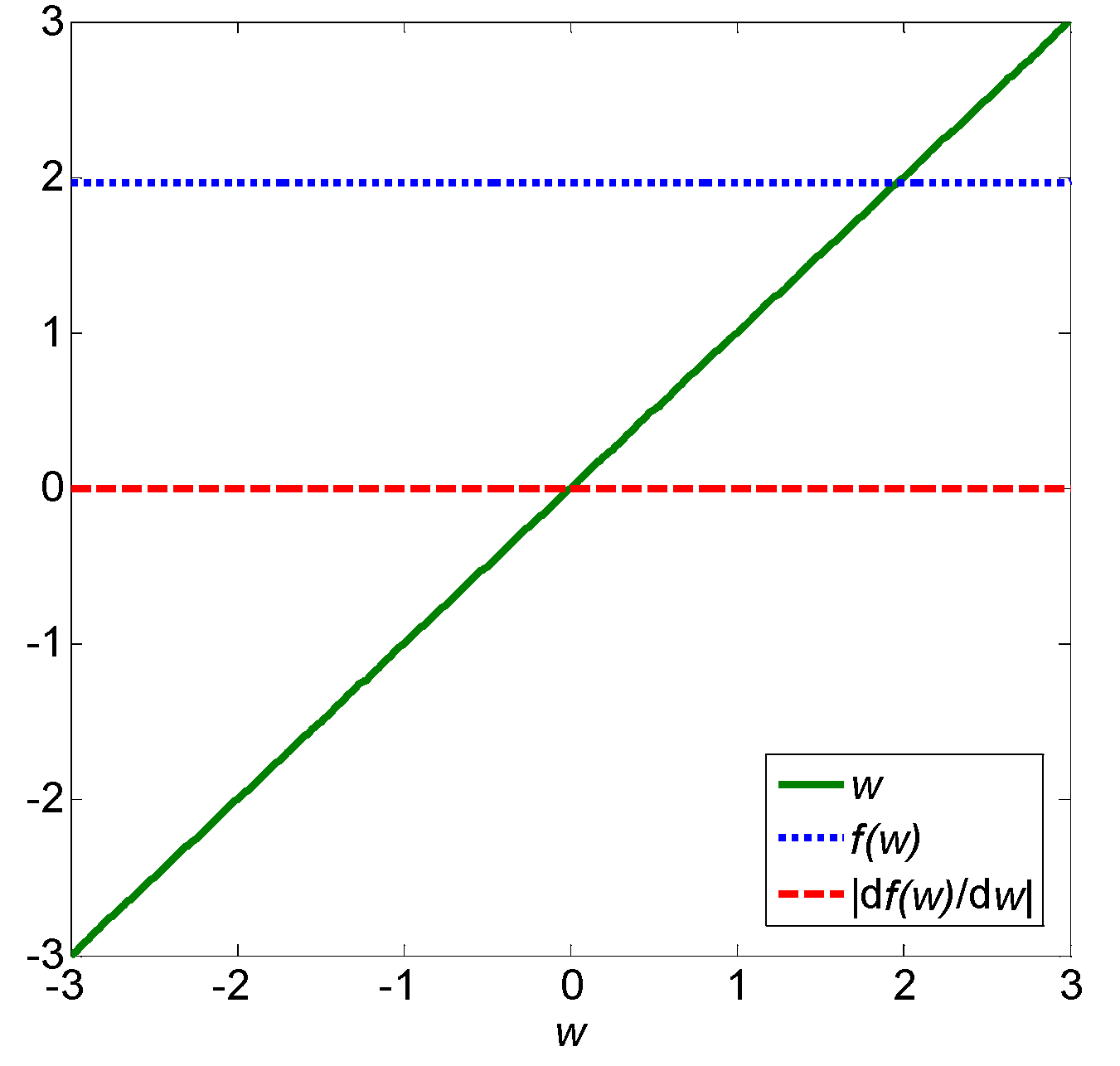
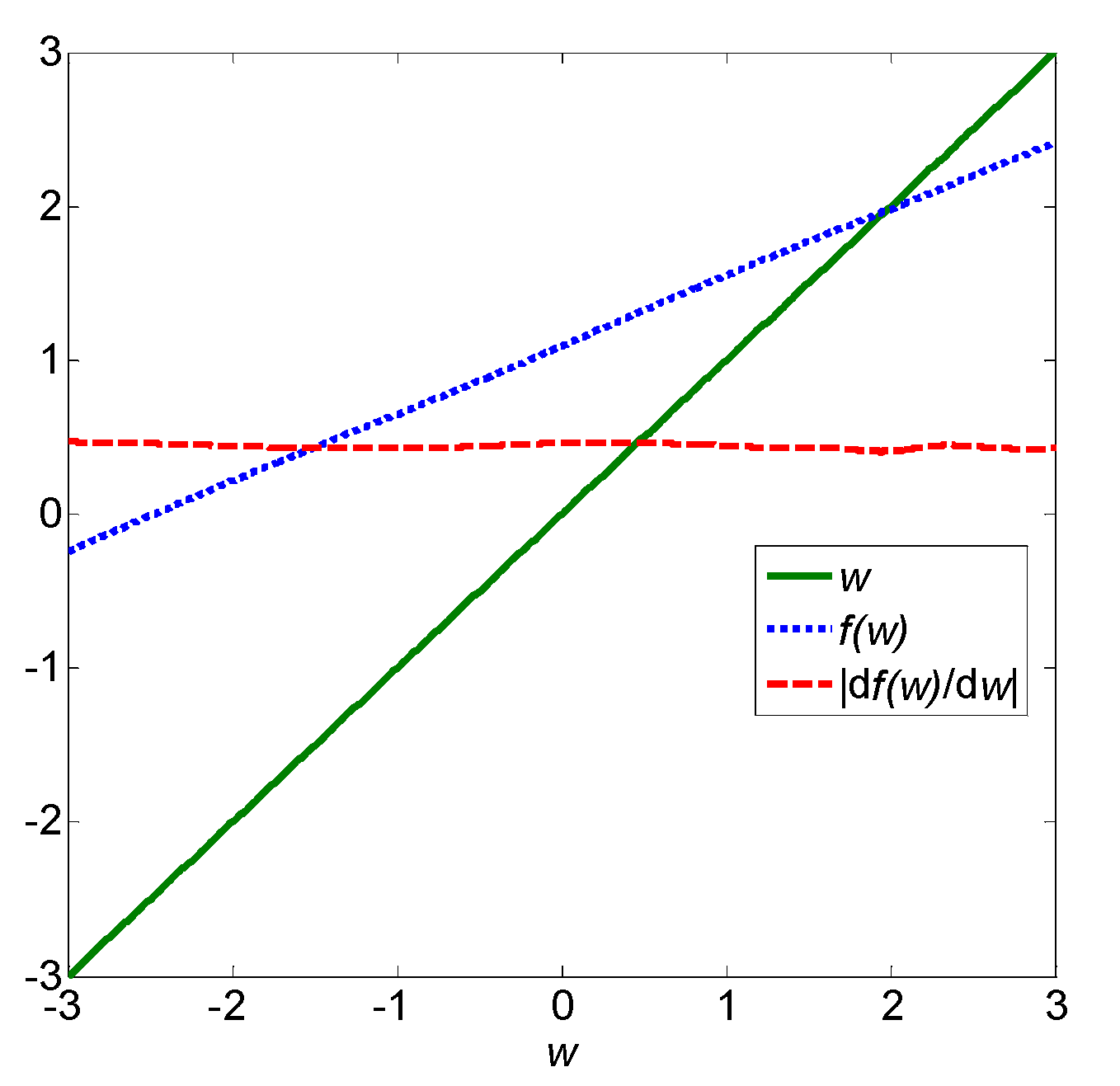
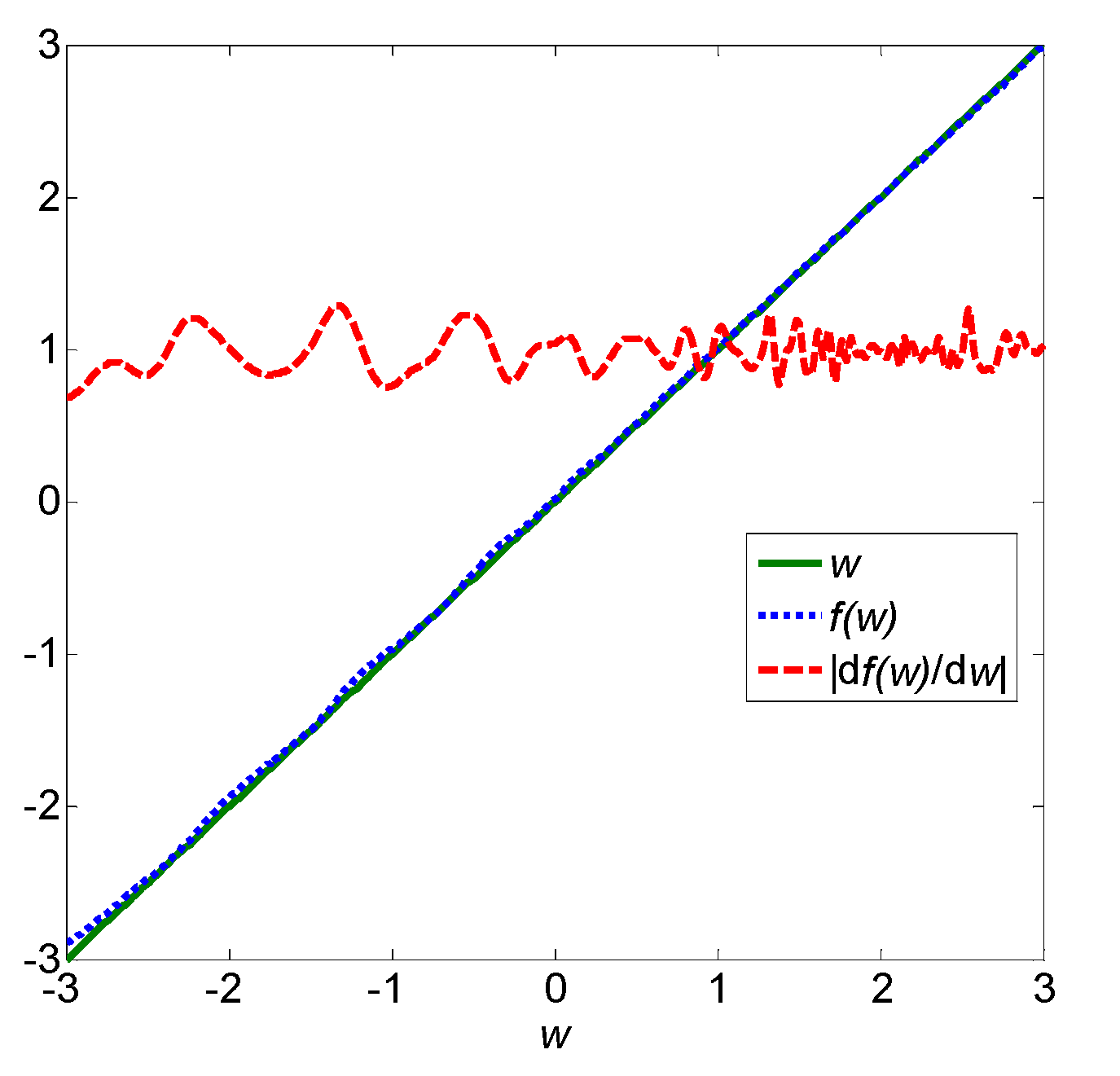
4. Illustrative Example

In the following, we give an illustrative example to verify the derived sufficient condition that guarantees the convergence of the fixed-point MEE algorithm. Let us consider a simple linear model:

$$d(i)=2X(i)+v(i)$$

(28)

where $X(i)$ is a scalar input, and $v(i)$ is an additive noise. Assume that $X(i)$ is uniform distributed over $\left[-\sqrt{3},\sqrt{3}\right]$ and $v(i)$ is zero-mean Gaussian with variance $0.01$. There are 100 training samples ${\left\{X(i),d(i)\right\}}_{i=1}^{100}$ generated from the system (28). Based on these data we calculate

$$\xi =\frac{{\displaystyle \sum _{i=1}^{100}{\displaystyle \sum _{j=1}^{100}\left|d(i)-d(j)\right|\times \left|X(i)-X(j)\right|}}}{{\displaystyle \sum _{i=1}^{100}{\displaystyle \sum _{j=1}^{100}{\left|X(i)-X(j)\right|}^2}}}=1.9714$$

(29)

We choose $\beta =3>\xi$ and $\alpha =0.9938<1$. Then by solving the equations $\phi (\sigma )=\beta$ and $\psi (\sigma )=\alpha$, we obtain ${\sigma }^{\ast }=2.38$ and ${\sigma }^{†}=2.68$. Therefore, by Theorem 2, if $\sigma \ge 2.68$ the fixed-point MEE algorithm will converge to a unique solution in the range $-3\le W\le 3$. Figure 1, Figure 2 and Figure 3 illustrate the curves of the functions $W$, $\mathit{f}(W)={\left({\mathbf{R}}_{XX}^{MEE}\right)}^{-1}{\mathbf{P}}_{dX}^{MEE}$, and $\left|\frac{d\mathit{f}(W)}{dW}\right|$ when $\sigma =3.0$, $0.1$, $0.01$, respectively. From the Figures we observe: (i) when $\sigma =3.0>2.68$, we have $\left|\mathit{f}(W)\right|<3$ and $\left|\frac{d\mathit{f}(W)}{dW}\right|<\alpha$ for $-3\le W\le 3$; (ii) when $\sigma =0.1<2.68$, we still have $\left|\mathit{f}(W)\right|<3$ and $\left|\frac{d\mathit{f}(W)}{dW}\right|<\alpha$ for $-3\le W\le 3$. In this case, the algorithm still will converge to a unique solution in the range $-3\le W\le 3$. This result confirms the fact that the derived sufficient condition is a little loose (i.e., far from being necessary). The main reason for this is that there is a lot of zooming out in the derivation process; (iii) however, when $\sigma$ is too small, say $\sigma =0.01$, the condition $\left|\frac{d\mathit{f}(W)}{dW}\right|<\alpha$ will not hold for some $W\in \left\{-3\le W\le 3\right\}$. In this case, the algorithm may diverge.

Figure 1. Plots of the functions $W$, $\mathit{f}(W)$ and $\left|\frac{d\mathit{f}(W)}{dW}\right|$ when $\sigma =3.0$.

Figure 1. Plots of the functions $W$, $\mathit{f}(W)$ and $\left|\frac{d\mathit{f}(W)}{dW}\right|$ when $\sigma =3.0$.

Figure 2. Plots of the functions $W$, $\mathit{f}(W)$ and $\left|\frac{d\mathit{f}(W)}{dW}\right|$ when $\sigma =0.1$.

Figure 2. Plots of the functions $W$, $\mathit{f}(W)$ and $\left|\frac{d\mathit{f}(W)}{dW}\right|$ when $\sigma =0.1$.

Figure 3. Plots of the functions $W$, $\mathit{f}(W)$ and $\left|\frac{d\mathit{f}(W)}{dW}\right|$ when $\sigma =0.01$.

Figure 3. Plots of the functions $W$, $\mathit{f}(W)$ and $\left|\frac{d\mathit{f}(W)}{dW}\right|$ when $\sigma =0.01$.

Table 1 shows the numbers of iterations for convergence with different kernel bandwidths (3.0, 1.0, 0.1, 0.05). The initial weight vector is set at $W_0=0.1$, and the stop condition for the convergence is

$$\left|\frac{W_k-W_{k-1}}{W_{k-1}}\right|<{10}^{-6}$$

(30)

As one can see, when $\sigma =3.0\ge \max \left\{{\sigma }^{\ast },{\sigma }^{†}\right\}$, the fixed-point MEE algorithm will surely converge to a solution with few iterations. When $\sigma$ becomes smaller, the algorithm may still converge, but the convergence speed will become much slower. Note that when $\sigma$ is too small (e.g., $\sigma =0.01$), the algorithm will diverge (the corresponding results are not shown in Table 1).

Table 1. Numbers of iterations for convergence with different kernel bandwidths $\sigma$.

$\sigma$	3.0	1.0	0.1	0.05
Iterations	3	4	16	43

Table 1. Numbers of iterations for convergence with different kernel bandwidths $\sigma$.

$\sigma$	3.0	1.0	0.1	0.05
Iterations	3	4	16	43

5. Conclusion

The MEE criterion has received increasing attention in signal processing and machine learning due to its desirable performance in adaptive system training especially with non-Gaussian data. Many iterative optimization methods have been developed to minimize the error entropy for practical use. But the fixed-point algorithms have been seldom studied, and in particular, too little attention has been paid to the convergence issue of the fixed-point MEE algorithms. This paper presented a theoretical study of this problem, and proved a sufficient condition to guarantee the convergence of a fixed-point MEE algorithm. The results of this study may provide a possible range for choosing a kernel bandwidth for MEE learning. However, the derived sufficient condition may give a much larger kernel bandwidth than a desired one due to the zooming out in the formula derivation process. In the future study, we will try to derive a tighter sufficient condition that ensures the convergence of thefixed-point MEE algorithm.

References

1. Principe, J.C. Information Theoretic Learning: Renyi’s Entropy and Kernel Perspectives; Springer: New York, NY, USA, 2010. [Google Scholar]
2. Chen, B.; Zhu, Y.; Hu, J.C.; Principe, J.C. System Parameter Identification: Information Criteria and Algorithms; Elsevier: Amsterdam, the Netherlands, 2013. [Google Scholar]
3. Silverman, B.W. Density Estimation for Statistics and Data Analysis; Chapman & Hall: New York, NY, USA, 1986. [Google Scholar]
4. Erdogmus, D.; Principe, J.C. An error-entropy minimization for supervised training of nonlinear adaptive systems. IEEE Trans. Signal Process. 2002, 50, 1780–1786. [Google Scholar] [CrossRef]
5. Erdogmus, D.; Principe, J.C. Generalized information potential criterion for adaptive system training. IEEE Trans. Neural Netw. 2002, 13, 1035–1044. [Google Scholar] [CrossRef] [PubMed]
6. Erdogmus, D.; Principe, J.C. Convergence properties and data efficiency of the minimum error entropy criterion in adaline traing. IEEE Trans. Signal Process. 2003, 51, 1966–1978. [Google Scholar] [CrossRef]
7. Chen, B.; Zhu, Y.; Hu, J. Mean-square convergence analysis of ADALINE training with minimum error entropy criterion. IEEE Trans. Neural Netw. 2010, 21, 1168–1179. [Google Scholar] [CrossRef] [PubMed]
8. Chen, B.; Principe, J.C. Some further results on the minimum error entropy estimation. Entropy 2012, 14, 966–977. [Google Scholar] [CrossRef]
9. Chen, B.; Principe, J.C. On the Smoothed Minimum Error Entropy Criterion. Entropy 2012, 14, 2311–2323. [Google Scholar] [CrossRef]
10. Marques de Sá, J.P.; Silva, L.M.A.; Santos, J.M.F.; Alexandre, L.A. Minimum Error Entropy Classification; Springer: London, UK, 2013. [Google Scholar]
11. Agarwal, R.P.; Meehan, M.; O’Regan, D. Fixed Point Theory and Applications; Cambridge University Press: Cambridge, UK, 2001. [Google Scholar]
12. Cichocki, A.; Amari, S. Adaptive Blind Signal and Image Processing: Learning Algorithms and Applications; Wiley: New York, NY, USA, 2002. [Google Scholar]
13. Regalia, P.A.; Kofidis, E. Monotonic convergence of fixed-point algorithms for ICA. IEEE Trans. Neural Netw. 2003, 14, 943–949. [Google Scholar] [CrossRef] [PubMed]
14. Fiori, S. Fast fixed-point neural blind-deconvolution algorithm. IEEE Trans. Neural Netw. 2004, 15, 455–459. [Google Scholar] [CrossRef] [PubMed]
15. Han, S.; Principe, J.C. A fixed-point minimum error entropy algorithm. In Proceedings of the 16th IEEE Signal Processing Society Workshop on Machine Learning for Signal Processing, Arlington, VA, USA, 6–8 September 2006; pp. 167–172.
16. Chen, J.; Richard, C.; Bermudez, J.C.M.; Honeine, P. Non-negative least-mean-square algorithm. IEEE Trans. Signal Process. 2011, 59, 5225–5235. [Google Scholar] [CrossRef]
17. Chen, J.; Richard, C.; Bermudez, J.C.M.; Honeine, P. Variants of non-negative least-mean-square algorithm and convergence analysis. IEEE Trans. Signal Process. 2014, 62, 3990–4005. [Google Scholar] [CrossRef]
18. Chen, B.; Wang, J.; Zhao, H.; Zheng, N.; Principe, J.C. Convergence of a fixed-point algorithm under Maximum Correntropy Criterion. IEEE Signal Process. Lett. 2015, 22, 1723–1727. [Google Scholar] [CrossRef]
19. Kailath, T.; Sayed, A.H.; Hassibi, B. Linear Estimation; Prentice Hall: Upper Saddle River, NJ, USA, 2000. [Google Scholar]