Entropy Minimization Design Approach of Supersonic Internal Passages

Abstract

Fluid machinery operating in the supersonic regime unveil avenues towards more compact technology. However, internal supersonic flows are associated with high aerodynamic and thermal penalties, which usually prevent their practical implementation. Indeed, both shock losses and the limited operational range represent particular challenges to aerodynamic designers that should be taken into account at the initial phase of the design process. This paper presents a design methodology for supersonic passages based on direct evaluations of the velocity field using the method of characteristics and computation of entropy generation across shock waves. This meshless function evaluation tool is then coupled to an optimization scheme, based on evolutionary algorithms that minimize the entropy generation across the supersonic passage. Finally, we assessed the results with 3D Reynolds Averaged Navier Stokes calculations.

1. Introduction

The specific power extraction in fluid machinery scales with the specific mass flow, reaching a maximum at sonic conditions. Based on the conservation of momentum through a fluid machine, it follows that the specific power increases with the flow velocity. Consequently, we are compelled to explore supersonic internal rotating passages. The design of such supersonic internal passages is governed by the existence of large shock losses and a restricted operational range [1,2]. In the 1950s, research was focused on steam turbine applications [3] and rocket propulsion systems [4]. Nowadays, supersonic turbine rotors with a subsonic axial Mach number are being used in several applications:

• Organic fluid Rankine cycles, in thermo-solar plants or waste heat energy recovery systems [5].
• Fast start up gas turbines [6].
• Turbopump turbines, as in the rocket engine Vulcain [4].

In the quest to develop more efficient and compact fluid machinery, we are designing internal passages with supersonic inlet axial conditions. These types of turbines are suitable for fluid machines that follow the modified Brayton cycles, with an isothermal heat addition process where the combustor presents a convergent shape [7,8]. In those engines, the turbine inlet Mach number is limited to values below unity [9], because those authors were unaware of the possible uses of turbines with supersonic inlet flows. By contrast, in a previous publication, we had explored the performance of a turbine passage that was designed considering the starting capabilities, and coolability, of the airfoil [10]. The presence of the blunt leading edge, was responsible for strong leading edge shock waves and, consequently, led to the reduction of isentropic efficiency. Figure 1a depicts the iso-Mach contour at mid-span for a supersonic turbine design, whereas Figure 1c shows the Mach number distribution along the pressure and suction side. Both representations prove the existence of supersonic flow in the passage. On the other hand, Figure 1b represents the attempt to use a conventional design with the same supersonic inlet Mach number. As a consequence of the high area contraction associated with this design, supersonic flow is not established in the passage (unstarted configuration). Hence, a normal shock wave occurs in the inlet of the numerical domain. As shown by the Mach number distribution (Figure 1c-bottom) only subsonic flow exists along the conventional design profile. In an engine application, such a design would lead to a tremendous entropy rise (Δs ≈ 440 KJ/(Kg K)) and eventually this shock wave would evolve towards the combustor. The present publication proposes a new approach to optimize the design of supersonic passages.

Figure 1. (a) Mach number iso-contour in a supersonic passage; (b) Mach number iso-contour in a subsonic passage; (c) Isentropic Mach number distribution along the two passages.

Figure 1. (a) Mach number iso-contour in a supersonic passage; (b) Mach number iso-contour in a subsonic passage; (c) Isentropic Mach number distribution along the two passages.

In the present paper, we present a new design methodology, which was evaluated with distinct design choices/objectives. The optimized geometries were ultimately assessed using Reynolds-Averaged Navier-Stokes calculations. Figure 2a shows the specific mass flow in function of the inlet Mach number. The supersonic operation allows three times more specific mass flow rate than the subsonic operation. Therefore, the frontal area of the turbine could be reduced, enabling more compact designs. Figure 2b depicts the main flow patterns that are present in a supersonic bladed passage. The blockage caused by the airfoil leading edges is responsible for the generation of a detached oblique shock wave that propagates through successive reflections along the passage. The shock waves cause an abrupt flow deviation, deceleration and entropy rise.

Figure 2. (a) Normalized specific mass flow rate at different inlet Mach number; (b) Flow pattern in a supersonic bladed passage.

Figure 2. (a) Normalized specific mass flow rate at different inlet Mach number; (b) Flow pattern in a supersonic bladed passage.

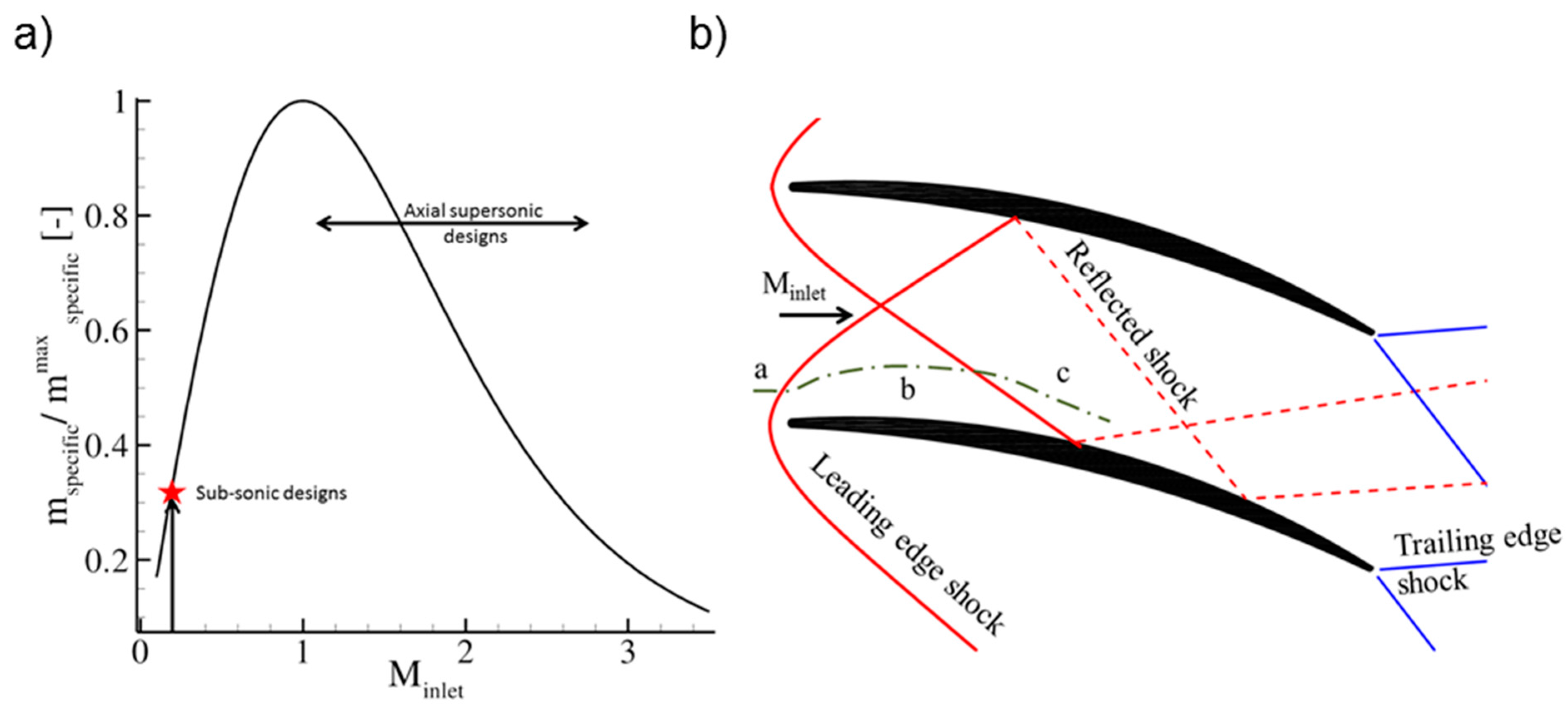
2. Allowable Turning through Supersonic Passages

The possible turning across bladed supersonic passages is restrained by the supersonic starting. At the beginning of the operation of a supersonic fluid machine, the flow will need to transit from a subsonic to a supersonic condition. During this unsteady starting process, a normal shock wave travels across the passage separating the subsonic from the supersonic domain. If this shock wave cannot be swallowed through the throat, the passage becomes unstarted. This results in tremendous aerodynamic losses and forces that jeopardize the aerodynamic and mechanical operation of the fluid machine. Kantrowitz and Donaldson [1] demonstrated that when this starting normal shock stands momentarily in front of the passage, flow with the post-normal shock conditions (M₂), as defined by Equation (1), enter the passage.

$$M_2^2=\frac{(\text{γ}-1)M_1^2+2}{2\text{γ}{M}_1^2-(\text{γ}-1)}$$

(1)

In order to ensure a started configuration, the entire subsonic mass flow rate must be allowed to proceed through the throat. Consequently, the area contraction of the converging passage must stand above the isentropic limit for the post shock flow conditions (at M₂). Equation (2) defines this isentropic area limitation, which is an exclusive function of the downstream subsonic Mach number (M₂) and the fluid properties.

$$\frac{A_{throat}}{A_{inlet}}=\frac{1}{M_2}{\left(\frac{2\left(1+(\text{γ}-1)/2)M_2^2\right)}{\text{γ}+2}\right)}^{-(\text{γ}+1)/(2(\text{γ}-1))}$$

(2)

Substituting Equation (1) into Equation (2) we define the Kantrowitz limit that ensures a started operation for any area reduction with contraction ratios larger than what is computed by Equation (3). The cross sectional area (A) of a perfectly axial machine is specified by the throat times the channel height (H), the area can then be expressed in function of the pitch (g), and the outlet metal angle (α): $A=g\times \cos (\text{α})\times H$.

$$\text{1}\frac{A_{throat}}{A_{inlet}}=\frac{g{H}_{throat}cos({\text{α}}_{throat})}{g{H}_{inlet}cos({\text{α}}_{inlet})}>\frac{1}{M_2}{\left(\frac{2\left(1+(\text{γ}-1)/2)M_2^2\right)}{\text{γ}+2}\right)}^{-(\text{γ}+1)/(2(\text{γ}-1))}$$

(3)

For a given inlet condition, the maximum possible outlet angle to ensure a started configuration can be evaluated using Equation (3). Figure 3 plots the maximum possible throat angle for a certain inlet Mach number (M₁) and inlet angle. Let us consider a fully inlet axial flow (α_inlet = 0) when M_ref = M_inlet = 2.0. The maximum turning through this particular passage would be limited to 34 (deg.). In case the inlet Mach number would be augmented by 50%, a much higher turning could be achieved (α_throat could be 44 deg.). Conversely, for the same inlet Mach number, an increase of inlet flow angle allows an increase of the turning.

Figure 3. Maximum blade turning in function of the inlet angle (αinlet) and Mach number normalized by M_ref according to the Kantrowitz limit.

Figure 3. Maximum blade turning in function of the inlet angle (αinlet) and Mach number normalized by M_ref according to the Kantrowitz limit.

3. Numerical Flow Analysis Method

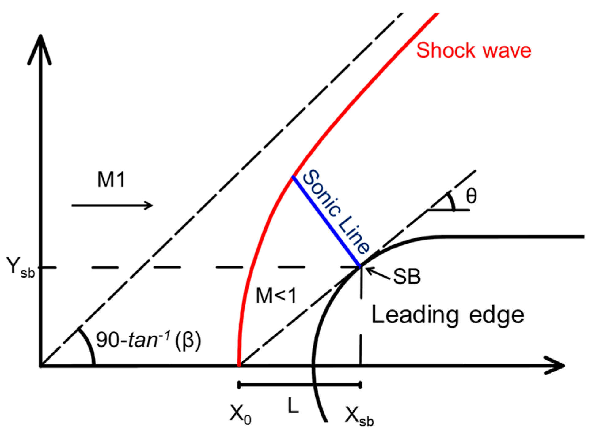
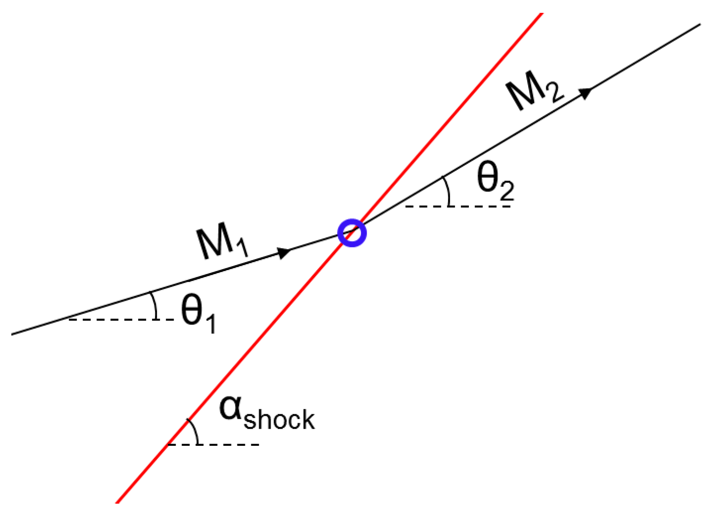
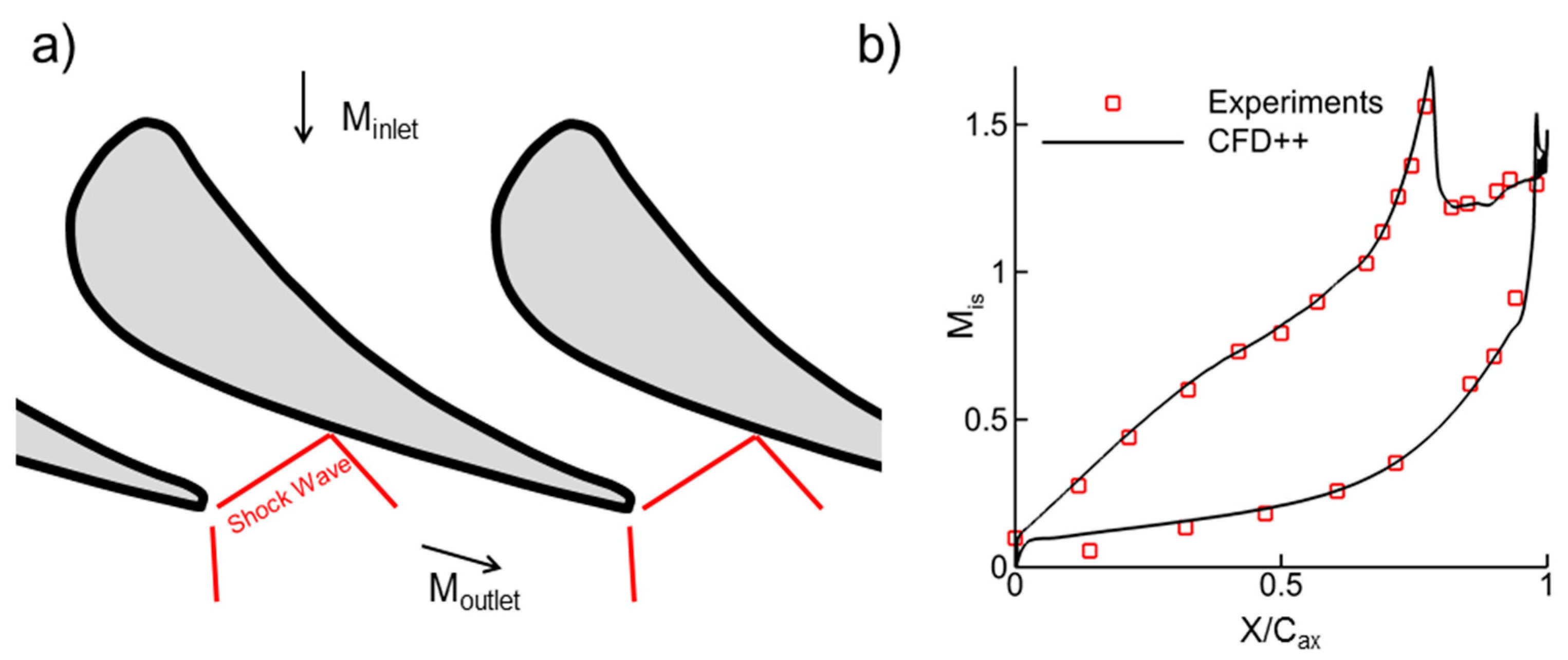
3.1. Leading Edge Shock Modeling

The leading edge shock waves were predicted using the empirical method developed by Moeckel [11] for inlet Mach numbers ranging between 1.1 and 3.5. Moeckel validated this approach for several leading edge shapes, including conical, spherical and projectile shapes.

Figure 4 sketches the shape of the leading edge shock wave, where point SB represents the sonic point on the airfoil surface while angle θ is the detachment angle for the incoming Mach number (M₁). The detached shock approximates to an asymptotic line for large distances from the leading edge. Hence, Moeckel proposed the use of a simple curve with the characteristics of a hyperbola represented by Equation (4) to define the wave shape.

$$y_{shock}=\frac{{\left(x_{shock}^2-x_0^2\right)}^{1/2}}{\text{β}}$$

(4)

Figure 4. Leading edge shock modeling.

Figure 4. Leading edge shock modeling.

In the current research the shape of the leading edge shock wave was compared with the CFD results at numerous inlet Mach numbers. Figure 5a presents a good agreement between the predicted shock wave (the red line), and with the CFD results visualized with numerical Schlieren (in grayscale). Figure 5b displays the entropy variation along the pitch-wise direction, across one passage (g, pitch) at three inlet Mach numbers. Most of the entropy is generated at the edge of the passage (Y = 0, or Y = g), where the leading edge shock is normal. Higher Mach numbers result in steeper gradients along the pitch-wise direction and a larger overall entropy generation.

Figure 5. (a) Numerical Schlieren at different inlet Mach numbers, red line represents the predicted/modeled leading edge shock wave, (b) leading edge shock losses prediction along the tangential direction at three inlet Mach numbers and comparison with CFD results

Figure 5. (a) Numerical Schlieren at different inlet Mach numbers, red line represents the predicted/modeled leading edge shock wave, (b) leading edge shock losses prediction along the tangential direction at three inlet Mach numbers and comparison with CFD results

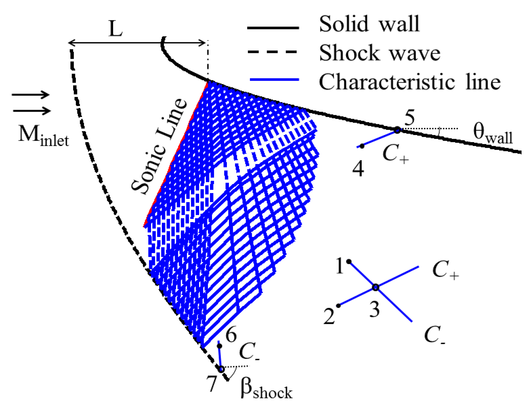
3.2. Method of Characteristics

The Method Of Characteristics (MOC) is a meshless approach with a limited computational demand. The procedure is applicable to the solution of any second-order hyperbolic partial differential equation [12]. Hence, it is suitable to the steady, two dimensional and irrotational flow. The resulting system of three equations (Equations (5)–(7)) has three unknowns: Φ_xx Φ_xy Φ_yy (Φ being the velocity potential).

$$\left(1-\frac{u^2}{a^2}\right){\text{Φ}}_{xx}+\left(1-\frac{v^2}{a^2}\right){\text{Φ}}_{yy}-\frac{2uv}{a^2}{\text{Φ}}_{xy}=0$$

(5)

$$d{\text{Φ}}_x={\text{Φ}}_{xx}dx+{\text{Φ}}_{xy}dy$$

(6)

$$d{\text{Φ}}_y={\text{Φ}}_{xy}dx+{\text{Φ}}_{yy}dy$$

(7)

The following step involves the determination of the direction along which the quantity Φ_xy is undetermined. These directions represent the lines where the derivative of the velocity is discontinuous, which are known as characteristic lines. The slope of this characteristic’s line at a certain point in the flow field can be determined with Equation (8).

$${\left(\frac{dy}{dx}\right)}_{char}=\text{tan}(\text{θ}\pm \text{μ})$$

(8)

where μ is the Mach angle given by μ = sin⁻¹(1/M) and θ is the flow direction at the evaluated location. Equation (8) stipulates that there are two characteristic lines passing through any point in the flow field. A left running characteristic that passes above the streamline (θ + μ known as C₊) and a right running one that passes below the streamline (θ − μ known as C₋). Along each of the characteristic line the flow properties are defined by the algebraic compatibility equations [12].

$$\text{θ}+v\left(M\right)=const=K_{-}(\text{along C}\_)$$

(9)

$$\text{θ}-v\left(M\right)=const=K_{+}(along{\text{ C}}_{+})$$

(10)

v(M) is the Prandtl-Meyer function for a certain local Mach number (M). In Figure 6, the lattice of characteristics begins at the sonic line. In order to avoid the singularity at M = 1 the flow velocity is set slightly above the sonic conditions (M = 1.1).

Figure 6. Different unit processes within the characteristic net of a 2D steady and irrotational flow.

Figure 6. Different unit processes within the characteristic net of a 2D steady and irrotational flow.

The calculations can then proceed in a marching manner. In point 3 (Figure 6), where two characteristics of opposite family (originated from two known points: 1 and 2) intersect the flow conditions can be computed by imposing: (K₋)₃ = (K₋)₁ and (K₊)₃ = (K₊)₂. When a boundary condition such as a solid wall is intersected (Point 5) the wall curvature should be equivalent to the flow direction (θ_wall = θ₅). Since, (K₊)₄ = (K₊)₅ point 5 can be easily computed. Another possible boundary condition is the downstream intersection with a shock wave, as depicted by point 7. The post shock conditions are estimated in an iterative manner by imposing (K₋)₆ = (K₋)₇ and using the oblique shock equations to find β_shock for a certain M_inlet that respects this equality [12].

When a characteristic intersects a downstream shock wave the oblique shock equations are used to estimate the post shock conditions, from where the marching method can be reestablished.

The entropy jump across the shock wave is evaluated at discrete locations. In particular, at the intersection of the characteristic line with this shock wave, as represented by the circular symbol in Figure 7.

Figure 7. Prior and post shock flow properties at the intersection with a characteristic line.

Figure 7. Prior and post shock flow properties at the intersection with a characteristic line.

Because the shock angle (α_shock), the upstream flow angle (θ₁) and upstream Mach number (M₁) are known, the computations of the temperature and pressure ratio across the shock can be obtained using Equations (11) and (12).

$$\frac{{\text{T}}_2}{{\text{T}}_1}=\frac{\left[2{\text{γM}}_1^2{\text{sin}}^2\left({\text{α}}_{\text{shock}}-{\text{θ}}_1\right)-(\text{γ}-1)\right]\left[\left(\text{γ}-1\right){\text{M}}_1^2{\text{sin}}^2\left({\text{α}}_{\text{shock}}-{\text{θ}}_1\right)+2\right]}{{\left(\text{γ}+1\right)}^2{\text{M}}_1^2{\text{sin}}^2({\text{α}}_{\text{shock}}-{\text{θ}}_1)}$$

(11)

$$\frac{{\text{P}}_2}{{\text{P}}_1}=\frac{2{\text{γM}}_1^2{\text{sin}}^2\left({\text{α}}_{\text{shock}}-{\text{θ}}_1\right)-(\text{γ}-1)}{\text{γ}+1}$$

(12)

The first time the flow crosses the leading edge shock wave (a to b in Figure 2b) the upstream flow properties are set by the inlet condition. At the second shock intersection (b to c in Figure 2b) θ₁ and M₁ are given by the upstream intersecting characteristic. At both crossings, α_shock is given by the Moeckel method. By contrast, at the remaining intersections, the angle of the shock wave is calculated by the shock-reflection prediction at the wall. Hence, the local entropy production at each intersection can then be calculated with Equation (13) and afterward average in the pitch-wise direction with Equation (14). The outlet entropy value is the addition of all the average values (a to b and b to c in Figure 2b).

$$\Delta {\text{s}}_{\text{local}}={\text{c}}_{\text{p}}\text{ln}\frac{{\text{T}}_2}{{\text{T}}_1}-\text{Rln}\frac{{\text{p}}_2}{{\text{p}}_1}$$

(13)

$$\Delta {\text{s}}_{\text{average}}=\frac{1}{\text{g}}\underset{0}{\overset{\text{g}}{{\displaystyle \int }}}\Delta \text{s}(\text{y})\text{dy}$$

(14)

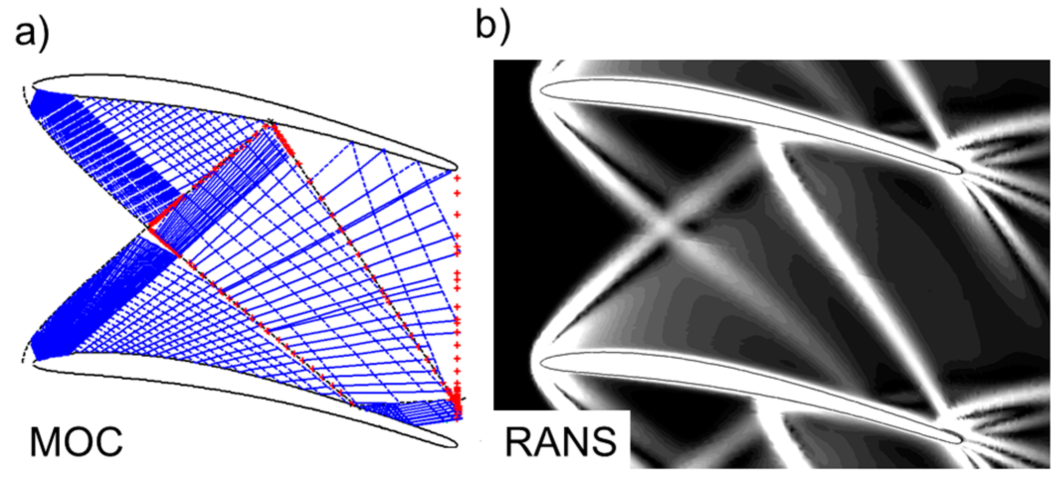
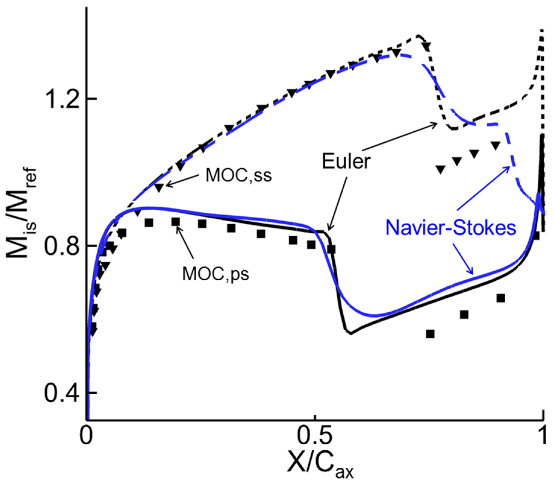
3.3. Assessment of the Method of Characteristics

The proposed flow evaluation tool was compared with current Reynolds-average Navier Stokes equations (RANS) methodologies. In particular, we used the commercial solver CFD++ version 14.1 developed by Metacomp Technologies, Agoura Hills, USA. Figure 8 displays the geometry investigated and the lattice of characteristics across the supersonic passage. The dotted (red) symbols over the shock waves represent the points where a characteristic crossed a shock wave. At these locations the oblique shock equations are used to compute the post shock flow conditions, and the entropy generation at each point. The area average entropy is then computed for each shock wave. The dots located at the passage outlet indicate where the outlet flow properties were evaluated. The numerical Schlieren visualization of the CFD results compares well with the present predictions.

Figure 8. (a) Illustration of the characteristic net and the empirically predicted shock waves. (b) Numerical Schlieren visualization obtained with 3D RANS simulations.

Figure 8. (a) Illustration of the characteristic net and the empirically predicted shock waves. (b) Numerical Schlieren visualization obtained with 3D RANS simulations.

Figure 9 presents the isentropic Mach number distribution along the pressure side and suction side using three different approaches: The 2D method of characteristics, 3D Euler simulations, 3D Reynolds Averaged Navier-Stokes simulations. The three methods present similar values within 2% of the reference Mach number except in the rear suction side. At x/C_ax = 0.75 the leading edge shock wave from the neighboring airfoil impacts with the boundary layer and therefore a separation bubble appeared, which results in a smoother variation of the Mach number, as described by the RANS simulations. By contrast, both Euler and MOC were unable to capture such a shock-boundary layer interaction and therefore they present a very steep variation.

The comparison of the Euler and RANS results allowed to quantify the viscous contribution to the entropy generation. In the present case, at high inlet supersonic conditions, the viscous effects only increased the total losses by 5%. In fact the prime contribution to the entropy generation was the shock loss, responsible for 70% of the total amount of entropy rises. The remaining 30% was split between profile, mixing and secondary loss. Consequently, in the present case, the method of characteristics, which neglects the viscous contribution, is an appropriate tool to optimize the airfoil profile, towards more efficient designs.

Table 1 compares the main outlet properties as the computed with both methods. In particular the total pressure loss, the average outlet Mach number and flow angle. From all the quantities of interest, the outlet flow angle is the one with the highest uncertainty, close to 4.7%. The computational time for both methods is also compared, where the proposed methodology requires only 0.5% of the computational time of 3D RANS simulations. The viscous effects, such as the boundary layers and the additional mixing processes, are only present in the RANS simulation and therefore contribute to the discrepancy between both methods.

Figure 9. Comparison of the isentropic Mach number distribution using the 2D Method of Characteristics (MOC), 3D non-viscous simulations (Euler), and 3D Reynolds Averaged Navier-Stokes simulations (RANS) at mid span.

Figure 9. Comparison of the isentropic Mach number distribution using the 2D Method of Characteristics (MOC), 3D non-viscous simulations (Euler), and 3D Reynolds Averaged Navier-Stokes simulations (RANS) at mid span.

Table 1. Comparison of the turbine outlet flow conditions computed with RANS and MOC simulations and the respective computational time.

	P0out/P0in [-]	Mout [-]	Θout [deg.]	Time [s]
Error	+4.7%	+0.6%	2[deg.]	−99.5%

Table 1. Comparison of the turbine outlet flow conditions computed with RANS and MOC simulations and the respective computational time.

	P0out/P0in [-]	Mout [-]	Θout [deg.]	Time [s]
Error	+4.7%	+0.6%	2[deg.]	−99.5%

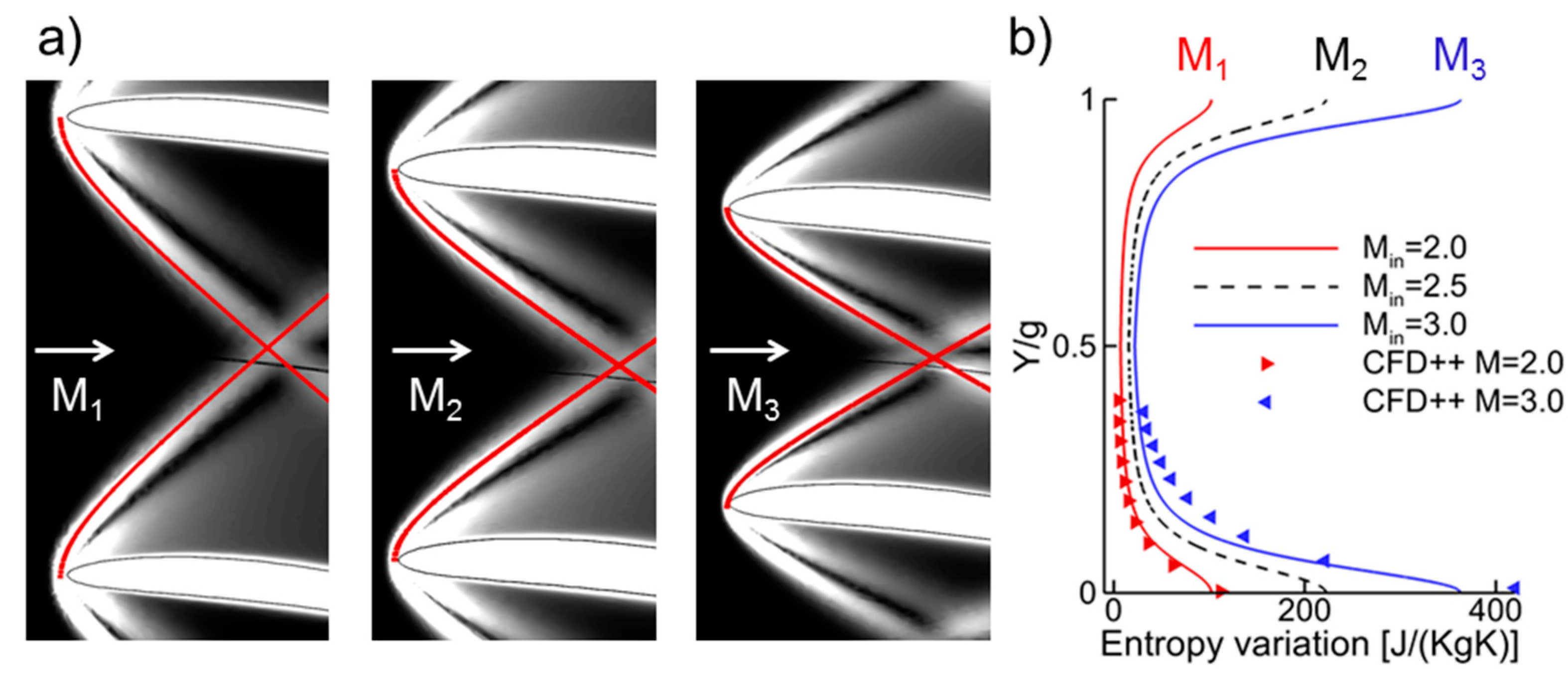
3.4. Numerical Tool Validation

The RANS solver, CFD++, was assessed using experimental data from a transonic nozzle guide vane [13]. The stator has 43 vanes with an axial chord of 41 mm. The turbine was operated at a pressure ratio (P₀₁/P_s3 = 3.8) that lead to a supersonic vane outlet Mach number (M_2is = 1.24). Static pressure measurements were performed along the stator pressure and suction side. In this assessment our computational 3D mesh has four million cells, which ensured a y⁺ below 1 in all the walls, necessary to resolve the laminar sublayer. Turbulent simulations were performed with the Spalart-Allmaras (SA) turbulence model. Figure 10a shows a 2D cut that sketches the impingent of the trailing edge shock wave on the suction side. Figure 10b shows a good agreement between the experimental isentropic Mach number and the numerical result obtained with CFD++. The solver adequately predicted the trailing edge shock impingement and its impact on the velocity field.

Figure 10. (a) 2D cut of the geometry used for validation purposes with representation of the trailing edge shock system. (b) Comparison between the experimental [13] and numerical isentropic Mach number across the passage at mid-span.

Figure 10. (a) 2D cut of the geometry used for validation purposes with representation of the trailing edge shock system. (b) Comparison between the experimental [13] and numerical isentropic Mach number across the passage at mid-span.

4. Supersonic Design Approach

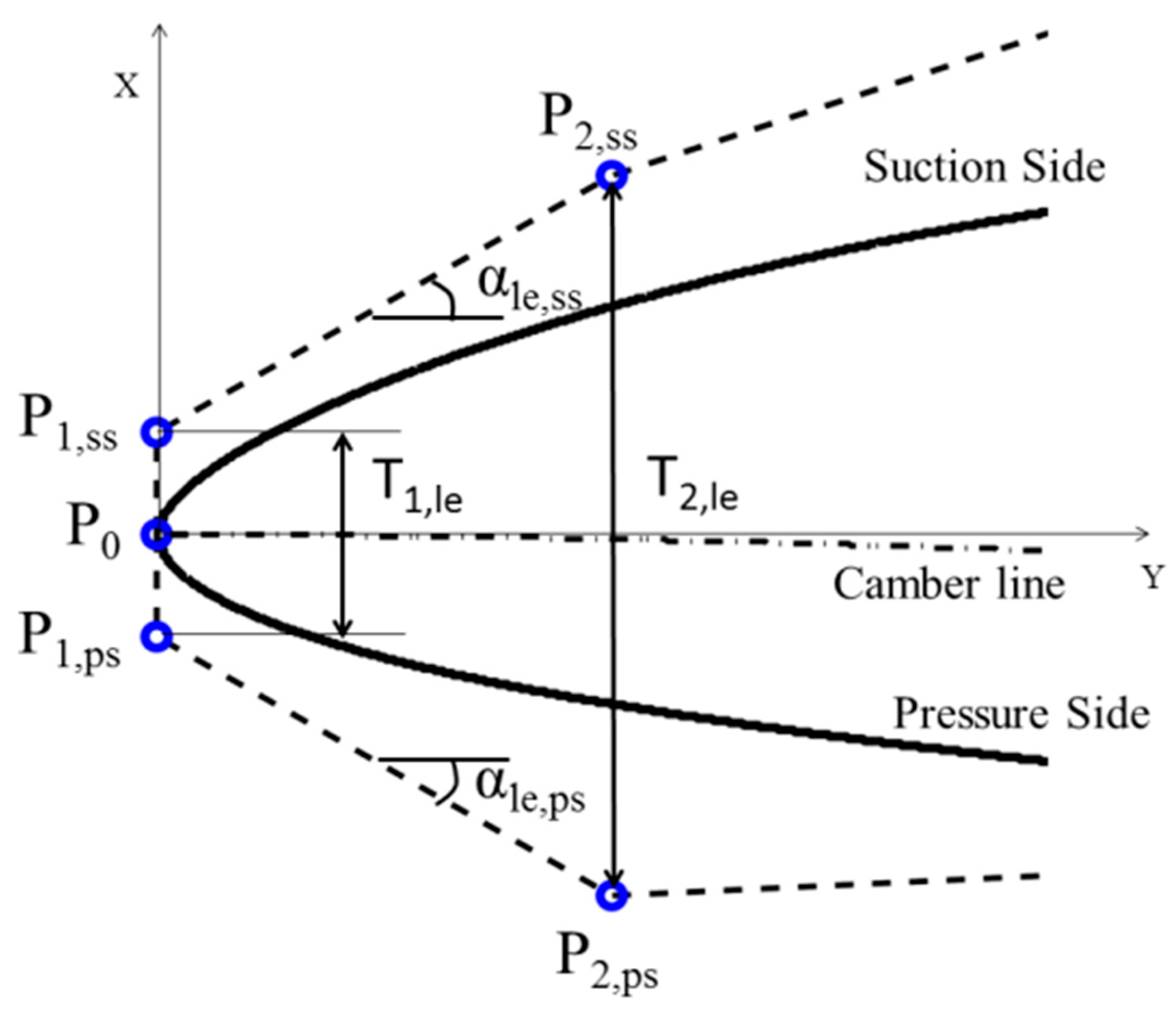
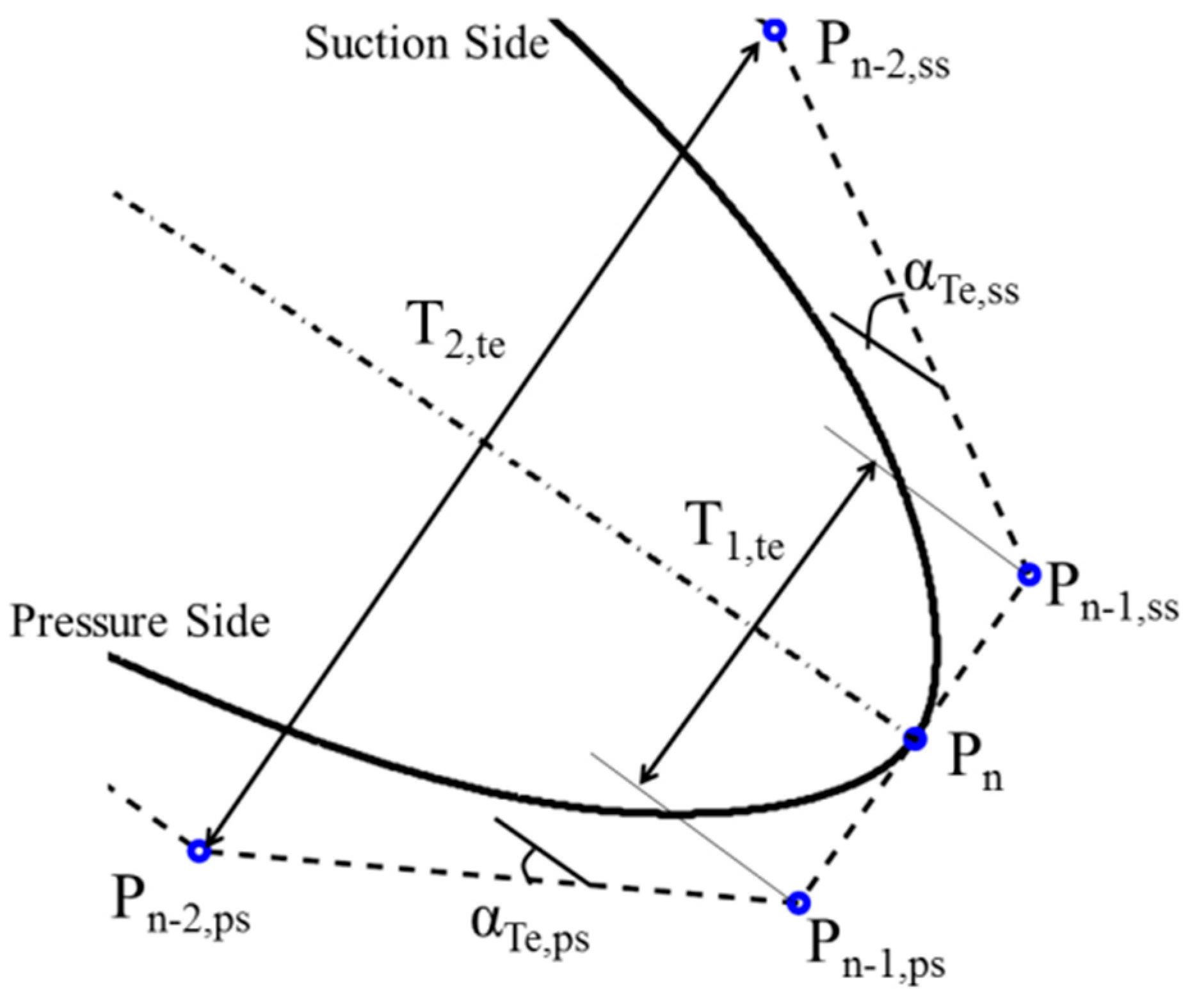
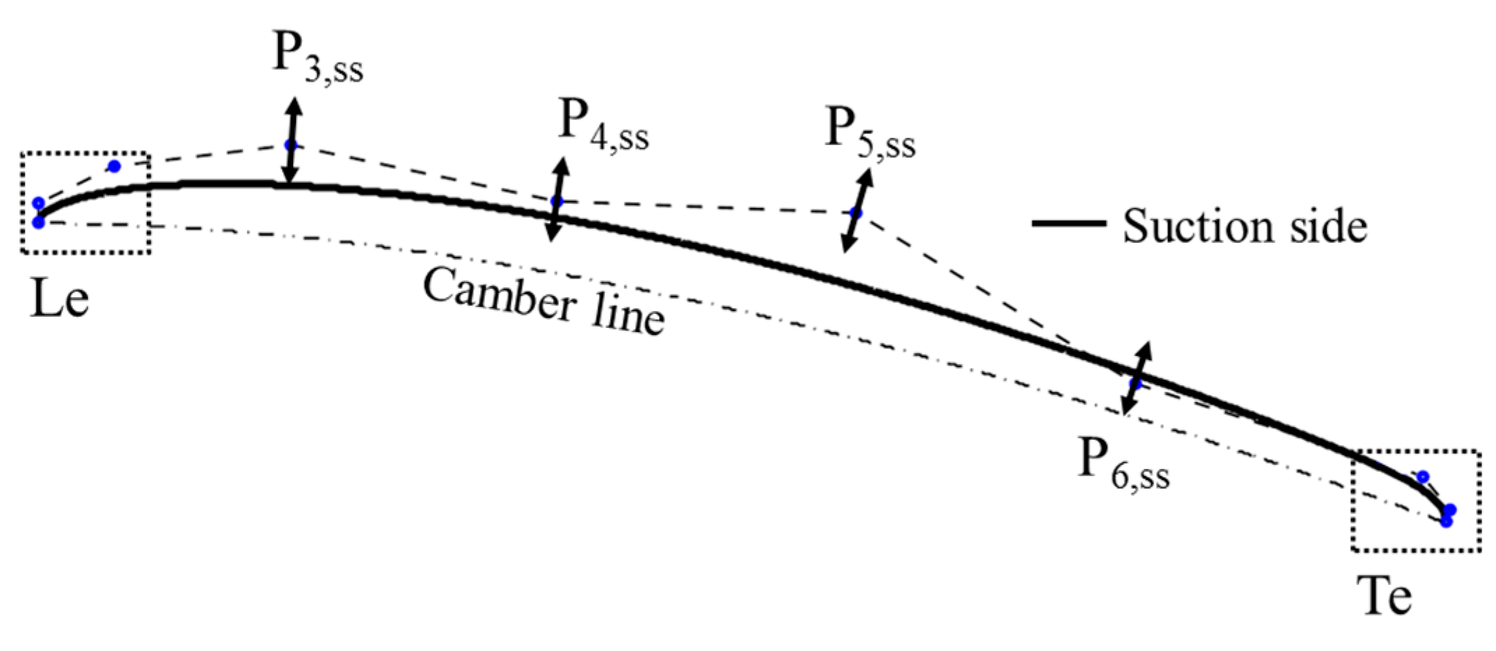
4.1. Geometrical Parameterization

The design procedure begins by defining the chord to pitch ratio and inlet-outlet metal angles. The camber line is constructed with a quadratic Bezier curve, where the first and last control points are placed at the leading and trailing edge.

Sharp leading edges are not allowed due to mechanical consideration. In order to reduce the leading edge shocks, several authors [14,15] proposed wedge-type geometries. Figure 11 represents our proposed leading edge parameterization. The free design parameters are:

-

the leading edge thicknesses (T_1,le)

-

the second leading edge thickness (T_2,le)

-

and the wedge leading edge angle (α_le)

Figure 11. Leading edge parameterization.

Figure 11. Leading edge parameterization.

Likewise, the trailing edge is defined in Figure 12 using:

-

the first trailing edge thickness (T_1,te)

-

the wedge trailing edge angle (α_Te)

-

the second trailing edge thickness (T_2,te)

Figure 12. Trailing edge parameterization.

Figure 12. Trailing edge parameterization.

The suction and pressure side are then built with Bezier curves. As illustrated in Figure 13, the control points are equally spaced in the axial direction and are then defined by its normal distance (thickness) to the camber line. The number of control points to define PS and SS, which is a free design parameter, is four in the present work. The proposed parameterization guarantees continuity in the local curvature of the leading up to the trailing edge of the airfoil.

Figure 13. Suction side parameterization.

Figure 13. Suction side parameterization.

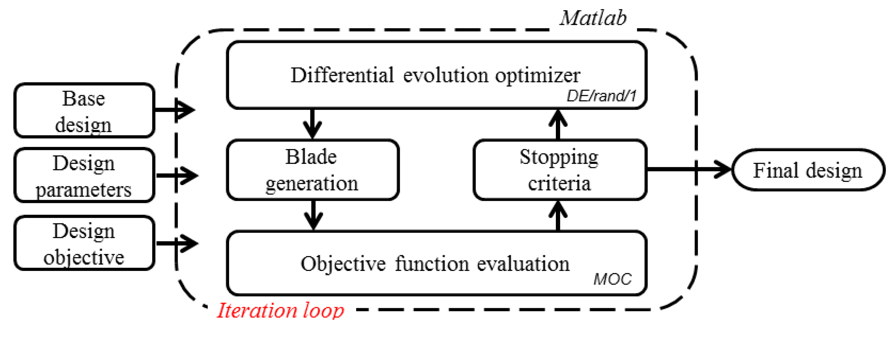
4.2. Optimization Approach

Evolutionary Algorithms (EA) were proposed and developed by Holland [16] in the 1970s. These algorithms follow the Darwinian theory of evolution, where several individuals form a population that evolves in time, following successive adaptations to their environment. The better fitted individuals have more likelihood to be retained (survive) and, thus, to reproduce. The population diversity and evolution is a consequence of mutation, crossover and finally of natural selection. In contrast to gradient based methods, evolutionary algorithms do not require having a continuous objective function, and additionally are more tolerant to noise [17]. Additionally, they are able to identify the global optima and avoid getting captured in a local minimum. The main drawback of evolutionary algorithms is the broad number of function evaluations required. However, as proposed in the present research, this issue can be addressed by using a fast function evaluation tool used to compute the objective function.

The chosen optimization strategy is the differential evolution approach named DE/rand/1 by Price and Storn [18]. This scheme is commonly used in turbomachinery applications [19] and the MATLAB code is openly available from Reference [20]. The weighting factor was set to F = 0.6, while the crossover probability to CR = 0.9.

The differential evolution is a population based, stochastic function minimizer. As shown in Figure 14, each time the method requires the evaluation of the objective function for a certain individual (in this case a certain passage), the method of characteristics is called within the optimization loop.

Figure 14. Diagram of the design/optimization process.

Figure 14. Diagram of the design/optimization process.

Several design options can be targeted depending on the chosen objective function. Additionally, several constrains can be imposed, such as a minimum mechanical thickness or a certain minimum flow turning.

The original population is randomly generated based on an initial geometry, where 10 different design variables were free to be modified within the limiting bounds summarized in Table 2. The control points of the initial geometry correspond to the mean level of these values.

Table 2. Bounded design space used by the optimizer.

Parameter	Lower–Upper SS	Upper–Lower PS
αle [deg.]	22.5–27.5	22.5–27.5
P3 [mm]	1.04–2.4	−1.9–6.1
P4 [mm]	1.29–4.9	−4.4–3.6
P5 [mm]	1.6–8.6	−3.1–4.9
P6 [mm]	−1.8–6.2	−3.2–4.8

Table 2. Bounded design space used by the optimizer.

Parameter	Lower–Upper SS	Upper–Lower PS
αle [deg.]	22.5–27.5	22.5–27.5
P3 [mm]	1.04–2.4	−1.9–6.1
P4 [mm]	1.29–4.9	−4.4–3.6
P5 [mm]	1.6–8.6	−3.1–4.9
P6 [mm]	−1.8–6.2	−3.2–4.8

5. Results of the Optimization Procedure

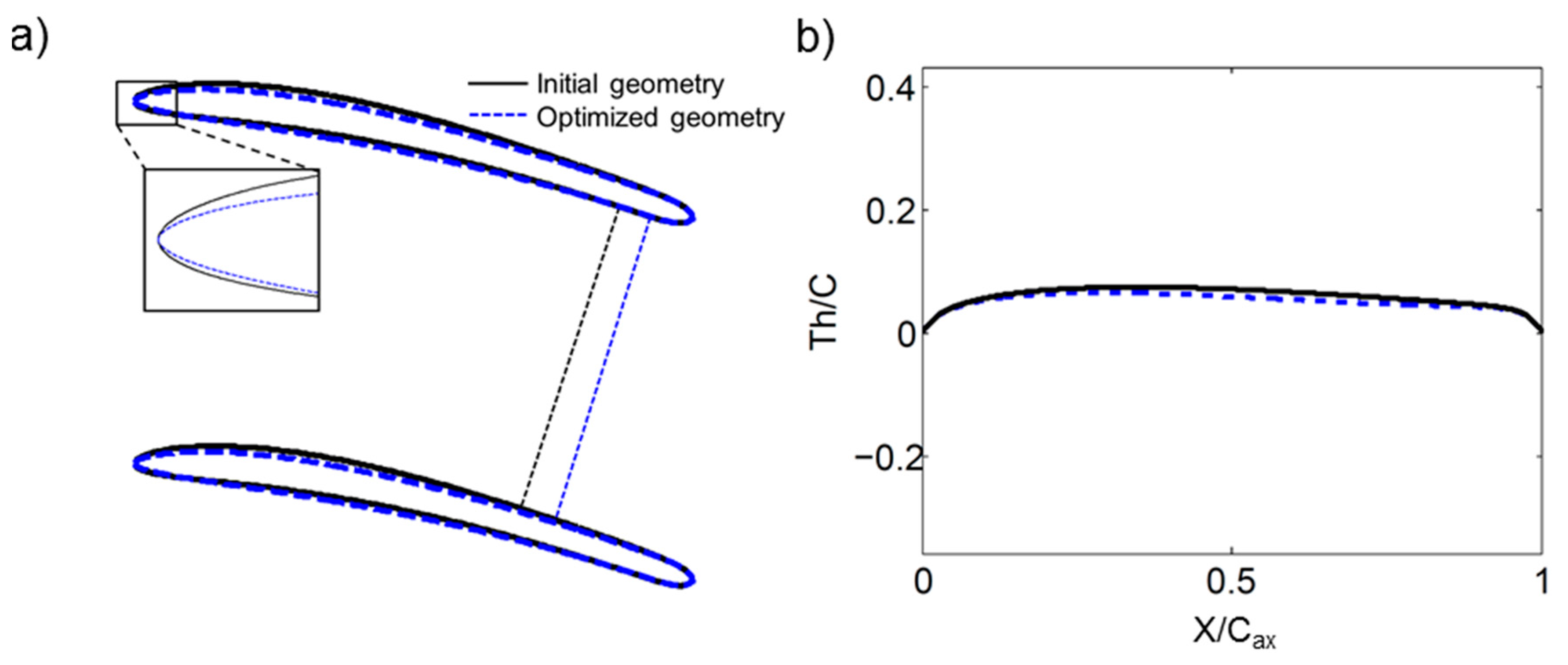
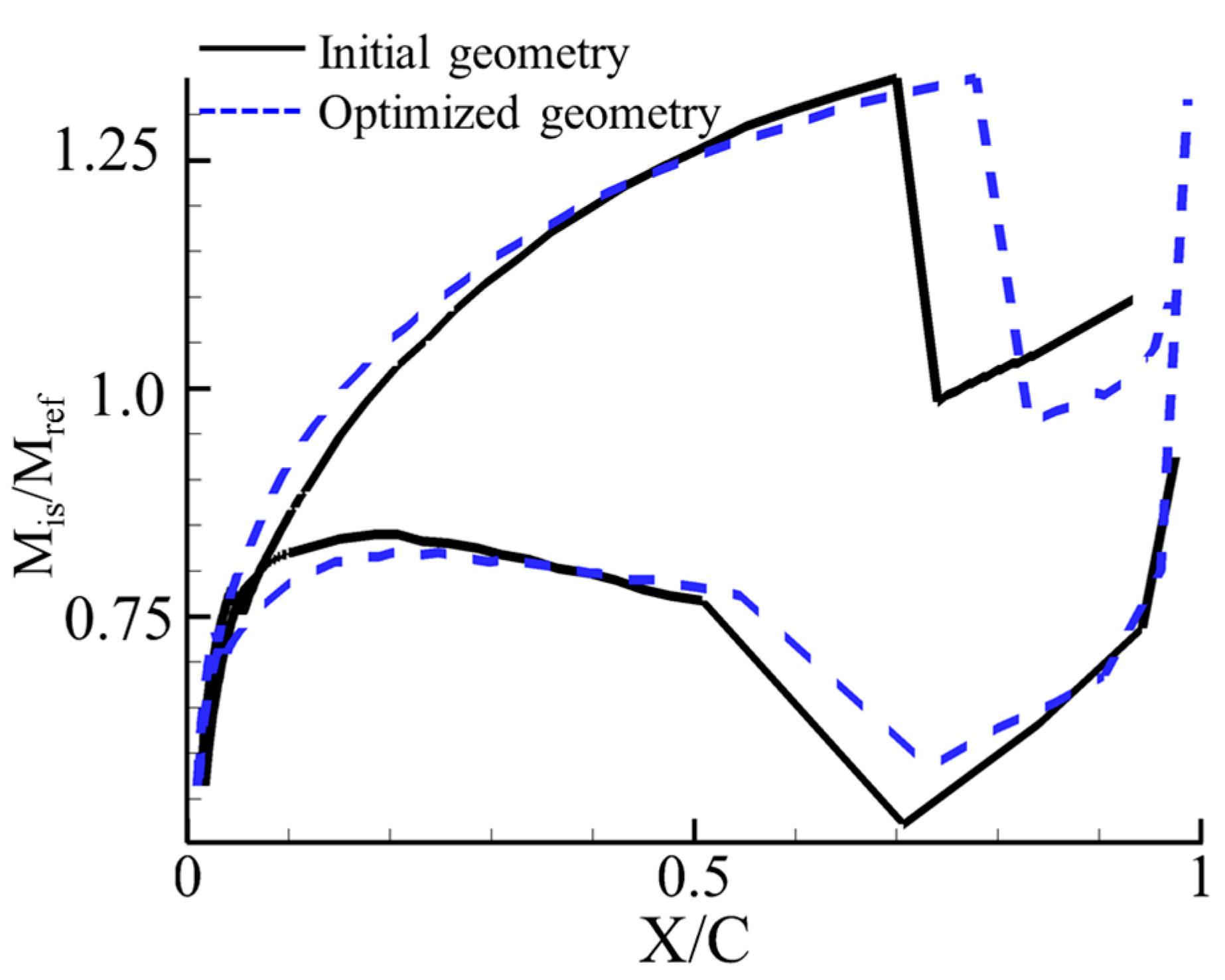
5.1. Minimum Losses

The first test case aimed the minimization of entropy production across the leading edge and reflected shock waves. Figure 15 displays the entropy evolution during the optimization process. After 36 iterations, the entropy generated by the supersonic passage was reduced by 15%. The initial and the optimized geometries were evaluated with the RANS solver of CFD++. The 3D calculations demonstrated the superiority of the optimized geometry. The outlet entropy was reduced 3.8 J/(KgK). This value represents a reduction of 6% of the total entropy production.

Figure 15. Entropy level at each iteration of the optimization process.

Figure 15. Entropy level at each iteration of the optimization process.

Figure 16a depicts the initial geometry (solid line) and the final optimized design (dashed line). The first thickness (T_1,le) was not altered to ensure a minimum leading edge thickness. Instead, the wedge angle (α_le,ss) was slightly reduced by 2.5 deg., and the second leading edge thickness (T_2,le) was lowered 16%. Consequently, the mechanical properties of the airfoil geometry were slightly modified. Table 3 lists the 2D cross section area (A), the minimum and the maximum momentum of inertia (I_min, I_max) and the angle between the axis of minimum momentum of inertia and the axial direction (α_Imin). Figure 16b shows the thickness distribution for both geometries along the axial direction. A maximum thickness difference occurred at X/C_ax = 50% where it was reduced by 10% in the optimized design. The resulting optimized profile allowed a reduction of the shock detachment distance, as well as a decrease of the shock angle relative to the flow, which consequently minimized the shock losses.

Figure 16. (a) Illustration of the initial profile shape (solid line) and the optimized one (dashed line) for minimum shock losses with detailed illustration of the leading edge modification. (b) Thickness variation along the axial direction for both geometries.

Figure 16. (a) Illustration of the initial profile shape (solid line) and the optimized one (dashed line) for minimum shock losses with detailed illustration of the leading edge modification. (b) Thickness variation along the axial direction for both geometries.

Table 3. Geometrical features of both geometries: 2D Area, minimum and maximum momentum of inertia and angle of the minimum momentum of inertia.

	A/g [m]	Imin [m4]	Imax [m4]	αImin [deg.]
Initial	9.57 × 10−3	3.02 × 10−9	4.37 × 10−7	−12.9
Optimized	8.34 × 10−3	1.02 × 10−9	3.84 × 10−7	−13.0

Table 3. Geometrical features of both geometries: 2D Area, minimum and maximum momentum of inertia and angle of the minimum momentum of inertia.

	A/g [m]	Imin [m4]	Imax [m4]	αImin [deg.]
Initial	9.57 × 10−3	3.02 × 10−9	4.37 × 10−7	−12.9
Optimized	8.34 × 10−3	1.02 × 10−9	3.84 × 10−7	−13.0

Figure 17 depicts the isentropic Mach number distribution along the suction and pressure side of the passage for both geometries. As illustrated in Figure 8b, the right and left running shock waves generated at the leading edge impact at the suction and pressure side, respectively. This interaction can be identified in Figure 17 where the flow velocity at the pressure side, around X/C_ax = 50% is notably reduced. The main differences between the initial and optimized designs are two-fold:

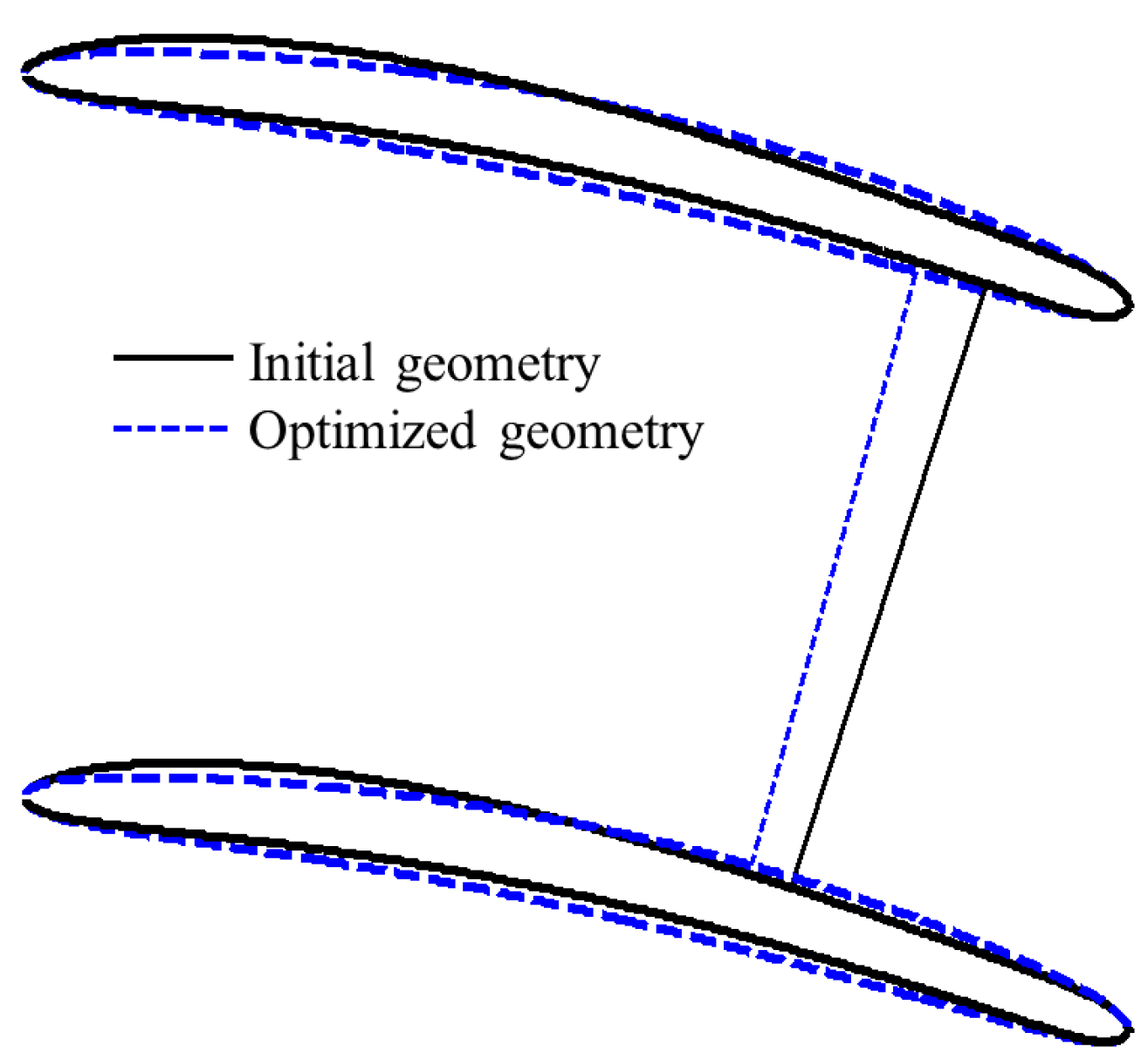
• A higher loading at the leading edge on the optimized geometry due to the greater flow acceleration on the suction side. The smoother acceleration along the pressure side helped to reduce the flow deceleration prior to the shock impact.
• Due to the smaller wedge angle of the leading edge, the shock waves have a higher inclination angle, which directly implies lower losses. As a consequence, the shock impact on the suction and pressure side occurs further downstream (10% of the suction side). Because the Mach number before the shock impingement is detrimental to the intensity of the reflected shock, the optimizer tried to reduce the upstream Mach number by modifying the suction side shape.

Figure 17. Isentropic Mach number distribution for the initial and the optimized geometry for minimum shock losses.

Figure 17. Isentropic Mach number distribution for the initial and the optimized geometry for minimum shock losses.

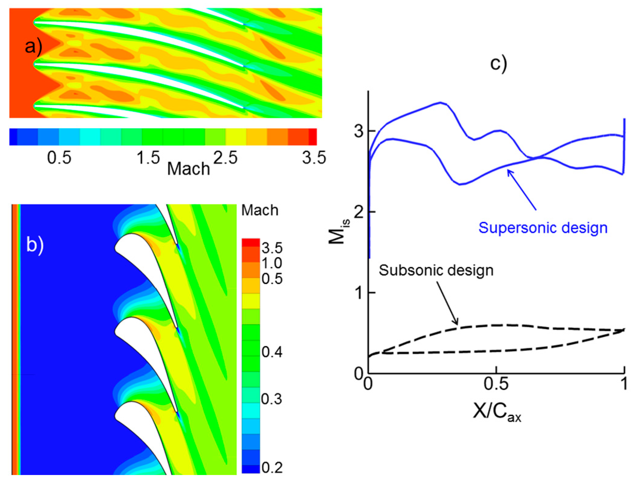
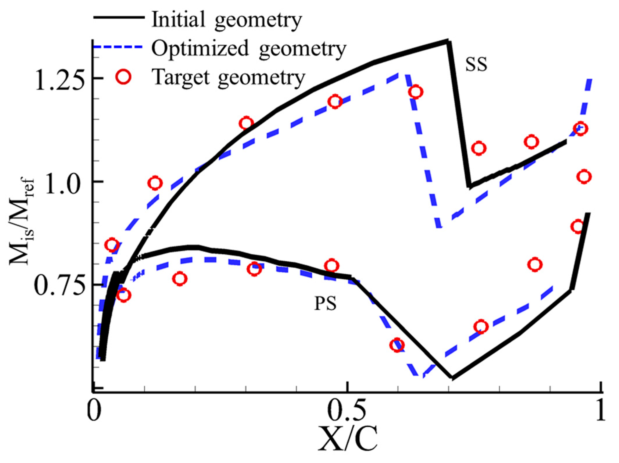
5.2. Imposed Mach Number Distribution

In this case the designer imposes a target velocity (or Mach number) distribution along the suction and pressure side of the passage. The optimizer will iteratively adjust the geometrical parameters and evaluate the overall difference in velocity between the target and the current profile. In this particular case the objective function is the minimization of such difference. Figure 18 displays the initial velocity profile (solid line) as well the target one (circular symbols). The target geometry was predefined to turn the flow more in the frontal part of the passage, where the boundary layer should be thinner, i.e., the target loading was increased in the front part. The rear suction side Mach number was decreased to reduce the pressure jump across the reflected shock in that region. The optimizer required 15 iterations to obtain the optimized geometry displayed in dashed lines.

Figure 18. Representation of the target Mach number distribution and respective initial and the optimized geometry.

Figure 18. Representation of the target Mach number distribution and respective initial and the optimized geometry.

Figure 19 compares the geometry of the initial profile and the modified one. One can observe that due to the higher targeted loading after the leading edge, both the suction and pressure side presents a higher curvature level. Additionally, due to the higher intended Mach number after the shock interactions, both the suction and pressure side present a more pronounced concave shape, that enhances the flow acceleration in this region.

Figure 19. Illustration of the initial profile shape and the optimized one that better fits the imposed Mach number distribution.

Figure 19. Illustration of the initial profile shape and the optimized one that better fits the imposed Mach number distribution.

6. Conclusions

This paper presents a design methodology for two-dimensional supersonic internal flow passages. The proposed design methodology provides a detailed parameterization of the leading edge where the greater part of the shock losses is generated. Additionally, the use of Bezier curves assures the curvature continuity from the leading to the trailing edge. The performance of the supersonic passage is evaluated by the method of characteristics. This flow evaluation tool was then coupled with an optimization routine with different design targets, one minimizing the entropy generation and another imposing a certain of the velocity distribution across the passage as objective function. The accuracy of the design method was then assessed with 3D Navier-Stokes solution, where the discrepancy between both methods was below 4.7% in predicting the losses. Additionally, the developed methodology requires only 0.5% of the Navier-Stokes computational time. This becomes of fundamental importance when using optimization algorithms, as implemented in the present work.

The numerical study yielded a deeper insight on the physics of supersonic flow passages and their design optimization. The research provides the knowledge to guide designers of future ultra-compact fluid machinery.

References

1. Kantrowitz, A.; Donaldson, C. Preliminary Investigation of Supersonic Diffusers; National Advisory Committee for Aeronautics: Washington, DC, USA, 1945. [Google Scholar]
2. Ferri, A. Preliminary Analysis of Axial-flow Compressors Having Supersonic Velocity at the Entrance of the Stator; National Advisory Committee for Aeronautics: Washington, DC, USA, 1949. [Google Scholar]
3. Verdonk, G.; Dufournet, T. Development of a Supersonic Steam Turbine with a Single Stage Pressure Ratio of 200 for Generator and Mechanical Drive; Von Karman Institute for Fluid Dynamics: Sint-Genesius-Rode, Belgium, 1987. [Google Scholar]
4. Whalen, U. The Aerodynamic Design and Testing of a Supersonic Turbine for Rocket Engine Application. In Proceedings of the 3rd European Conference on Turbomachinery Fluid Dynamics and Thermodynamics, London, UK, 2–5 March 1999.
5. Verneau, A. Supersonic Turbines for Organic Fluid Rankine Cycles from 3 to 1300 kw. Von Karman Institute for Fluid Dynamics: Sint-Genesius-Rode, Belgium, 1987. [Google Scholar]
6. Binsley, R.; Boynton, J. Aerodynamic Design and Verification of a Two-Stage Turbine with a Supersonic First Stage. J. Eng. Gas Turbines Power 1978, 100, 197–202. [Google Scholar] [CrossRef]
7. Tyagi, S.K.; Kaushik, S.C.; Tiwari, V. Ecological Optimization and Parametric Study of an Irreversible Regenerative Modified Brayton Cycle with Isothermal Heat Addition. Entropy 2003, 5, 377–390. [Google Scholar] [CrossRef]
8. Jubeh, N.M. Exergy Analysis and Second Law Efficiency of a Regenerative Brayton Cycle with Isothermal Heat Addition. Entropy 2005, 7, 172–187. [Google Scholar] [CrossRef]
9. Vecchiarelli, J.; Kawall, J.; Wallace, J. Analysis of a Concept for Increasing the Efficiency of a Brayton Cycle via Isothermal Heat Addition. Int. J. Energy Res. 1997, 21, 113–127. [Google Scholar] [CrossRef]
10. Paniagua, G.; Iorio, M.; Vinha, N.; Sousa, J. Design and Analysis of Pioneering High Supersonic Axial Turbines. Int. J. Mech. Sci. 2014, 89, 65–77. [Google Scholar] [CrossRef]
11. Moeckel, W. Approximate Method for Predicting form and Location of Detached Shock Waves ahead of Plane or Axially Symmetric Bodies; National Advisory Committee for Aeronautics: Washington, DC, USA, 1949. [Google Scholar]
12. Anderson, J.D. Modern Compressible Flow: With Historical Perspective; McGraw Hill Higher Education: New York, NY, USA, 1990. [Google Scholar]
13. Paniagua, G.; Yasa, T.; La Loma, A.D.; Castillon, L.; Coton, T. Unsteady Strong Shock Interactions in a Transonic Turbine: Experimental and Numerical Analysis. J. Propuls. Power 2008, 24, 722–731. [Google Scholar] [CrossRef]
14. Dvořák, R.; Šafařík, P.; Luxa, M.; Šimurda, D. Optimizing the Tip Section Profiles of a Steam Turbine Blading. In Proceedings of the ASME 2013 Turbine Blade Tip Symposium, Hamburg, Germany, 30 September–3 October 2013; p. V001T01A001.
15. Senoo, S. Development of Design Method for Supersonic Turbine Aerofoils near the Tip of Long Blades in Steam Turbines: Part 1—Overall Configuration. In Proceedings of the ASME Turbo Expo 2012: Turbine Technical Conference and Exposition, Copenhagen, Denmark, 11–15 June 2012; pp. 355–365.
16. Holland, J. Adaptation in Natural and Artificial Systems; University of Michigan Press: Ann Arbor, MI, USA, 1975. [Google Scholar]
17. Verstraete, T. CADO: A Computer Aided Design and Optimization Tool for Turbomachinery Applications. In Proceedings of the 2nd International Conference on Engineering Optimization, Lisbon, Portugal, 6–9 September 2010; pp. 6–9.
18. Storn, R.; Price, K. Differential Evolution—A Simple and Efficient Heuristic for Global Optimization over Continuous Spaces. J. Glob. Optim. 1997, 11, 341–359. [Google Scholar] [CrossRef]
19. Das, S.; Suganthan, P.N. Differential Evolution: A Survey of the State-of-the-Art. IEEE Trans. Evolut. Comput. 2011, 15, 4–31. [Google Scholar] [CrossRef]
20. Differential Evolution (DE) for Continuous Function Optimization (an algorithm by Kenneth Price and Rainer Storn). Available online: http://www1.icsi.berkeley.edu/~storn/code.html (accessed on 30 July 2015).