1. Introduction
Many systems in the world can be modeled by a network, that is a set of items (vertices) with connections between them (links) [
1]. Hence, the study of networks has been engaged in several branches of science. For example, in the mathematical form of graph theory, it is one of the fundamental grounds of discrete mathematics [
2]. Moreover, networks have also been extensively studied in social science [
3]. In recent years, network research moved from the analysis of single small graphs and the properties of individual vertices or links to the statistical properties of entire graphs [
4]. As a consequence, several different statistical mechanics tools have been conceived of in order to quantify the different levels of organization of real networks [
5]. Among them, entropic measures play a relevant role [
6]. Along this line, by resorting to methods of information geometry [
7], we have introduced recently a geometric entropy for Gaussian networks [
8], namely networks having Gaussian random variables sitting on vertices and their correlations as weighted links. Such network models, besides being rather easy to handle, find many applications, ranging from neural networks to wireless communication, from protein to electronic circuits,
etc.Traditionally, research on networks focused on features of static graphs. In this area, the study of topology networks is one of the most investigated issues. Although there is a wide diversity in the size and aim of networks observed in nature and technology, their topology shares several highly-reproducible and often universal characteristics [
9]. Yet, almost all real networks are dynamic in nature [
10]. Unfortunately, dealing with dynamic processes in network diversity prevails over the universality [
11], and each network dynamical process is studied on its own terms, requiring its dedicated analytical formalism and numerical tools.
In the context of Gaussian networks, it seems quite natural to consider the dynamics of involved random variables described by a (multivariate) Ornstein–Uhlenbeck process [
12]. In this way, the Gaussian character of the joint probability distribution is preserved over time. Taking this approach, we shall investigate how the evolution is reflected on the geometric entropy. Actually, we associate a Riemannian manifold endowed with a metric structure (that of Fisher–Rao) with the network at each time. Then, the change in level of organization of such an evolving system will be measured trough the change of the entropy, given by the logarithm of the volume of the manifold, when passing from one manifold to another.
As a simple case study, we shall consider a three-node Gaussian network. There, a first stochastic process will be considered with the aim of switching on all links starting from an uncorrelated Gaussian probability distribution (fully disconnected network). In contrast, a second stochastic process will be introduced aiming at switching off all links starting from a joint Gaussian probability distribution totally correlated (fully-connected network). The geometric entropy for these two cases varies monotonically as a function of time and shows a crossing behavior. Additionally, we shall deal with intermediate situations where part of the links are switched on and part switched off. In such cases, the geometric entropy no longer varies monotonically, while still exhibiting crossing behaviors between switched on and off links.
The layout of the article is as follows. In
Section 2, we describe the measure of complexity related to the volume of the Riemannian statistical manifold associated with a static Gaussian network. In
Section 3, we introduce the network dynamics, and we associate a manifold with the network at each time, thus providing a kind of foliation of the statistical manifold. Then, in
Section 4, we study various dynamical cases occurring in a network having three vertices and show how their features are reflected into the geometric entropy. At the end, in
Section 5, we draw our conclusions.
2. Statistical Models and Network Complexity Measure
We start considering
n real-valued random variables
with joint Gaussian probability distribution:
where
and
C is the
covariance matrix with entries
,
. Throughout the paper, we assume to deal with zero mean probability distribution functions.
The set of all (zero mean) Gaussian probability distributions turns out to be a statistical model when we consider each function parametrized by its covariances
,
. To be more precise, the function
in Equation (
1) can be uniquely characterized by
parameters
, with
for
and
when
. This amounts to number entries
of the covariance matrix
C when
. In such a way, we can rewrite
. Therefore, the set:
is called the
m-statistical multivariate (zero mean) Gaussian model on
as the mapping
is injective, and the parameter space is
[
7].
Given the statistical model
in Equation (
2), the mapping
defined by
is injective, and it allows us to consider
as a coordinate system for
. In addition, we assume that a change of coordinates
is such that the set
, where
κ is the set of new coordinates given by
, represents the same family of probability functions as
. Finally, if we consider
-differentiable changes of coordinates, then
can be considered as a
differentiable manifold, called a statistical manifold [
7].
Consider now a point
; then, the Fisher information matrix of
at
θ is the
matrix
, where the entries are given by:
with
standing for
and
running in the set
. The matrix
results in being symmetric and positive semidefinite. Yet, we assume from here on that
is positive definite. In such a way, we can endow the parameter space Θ with a Riemannian metric, the Fisher–Rao metric associated with the Gaussian statistical model
of Equation (
1), given by
, with
as in Equation (
3). Finally, the manifold
describes a Riemannian manifold.
At this point, we can interpret the random variables
as sitting on vertices of a network and their correlations as weighted links among the vertices of such a network. Thereby, thanks to the parametric characterization of the Gaussian probability
in Equation (
1), we can lift a network (discrete system) to a differentiable system (the Riemannian manifold
). To be more precise, we are considering random variables as hidden variables sitting on the vertices of an undirected network (without loops on its vertices), and their correlations are seen as weighted links among the vertices, again. Therefore, we are focusing the attention on the knowledge of some parameters characterizing the hidden variables. All of the information about the system is retained in these parameters. In particular, given the information on the variances and covariances of the multiple hidden variables, a multivariate Gaussian probability distribution describing the whole given network can be derived by means of the maximum entropy principle [
13]. Thus, a parameter space is associated with any given network. This space encodes all of the information about the structure of the associated network.
In order to quantify the degree of organization of a given network, it is quite natural to consider the volume of the associated Riemannian manifold. To this end, let us first consider the volume element of the manifold
,
Then, the volume
of
is evaluated as [
8]:
where
is a suitable regularizing function introduced to avoid the possibility of having an ill-defined volume. Since the parameter space Θ is quite generally not compact, the function
provides a kind of compactification of Θ by excluding the contributions of
, making
divergent. It is clear that the regularizing function depends on the characteristic of the space Θ, as well as on the functional form of
. An explicit expression of
has been devised in some particular cases [
8]. We are now in a position to define a complexity measure for a given network
with associated manifold
as:
The definition (
6) is inspired by the microcanonical definition of entropy in statistical mechanics [
14]. In fact, the latter involves the phase space volume bounded by the hypersurface of constant energy
E, which can be traced back to
, where
is a configuration space subset determined by
E,
q are the configuration coordinates and
is the Jacobi kinetic energy tensor.
Unfortunately, computing such a quantity results in being quite hard. In fact, from Equations (
1) and (
3), it follows that:
where the exponential stands for a power series expansion over its argument (the differential operator) and:
The derivative of the logarithm reads:
where
denotes the
entry of the inverse of the covariance matrix
C in (
1). The latter equation together with Equation (
7) show the computational complexity of Equation (
3). Indeed, the well-known formulas:
require the calculation of
derivatives with respect to the variables
in order to work out the derivative of the logarithm in (
9). Finally, to obtain the function
in (
8), we have to evaluate
derivatives. This quickly becomes an unfeasible task with growing
n, even numerically.
To overcome this difficulty, we consider only the variances of the random variables as local coordinates of the manifold associated with the network. This means that the elements of the parameter space Θ are:
In this way, the topological dimension of the manifold
reduces from
to
.
Thus, given a network
with
n vertices and the
adjacency matrix
A, consider the matrix
defined as:
with
. Here,
is the weighted
symmetric matrix associated with the network
, whose entries are given by:
where
is a real constant and
is the
i-th element of the canonical basis in
.
Finally, to the network
, we associate the parameter space:
There, we introduce a new metric
with components:
where
is the
entry of the inverse of the matrix
. This choice is motivated by the functional relation found in [
8] between the Fisher–Rao matrix elements and the covariance matrix elements when the latter takes values of zero or one out of the main diagonal.
It turns out that
is a Riemannian metric. Hence, with a given network
, we associate the Riemannian manifold
. Ultimately, we consider a statistical measure of the complexity of the network
with weighted matrix
W and associated manifold
as:
where
is the volume of
evaluated from the element:
with
the
symmetric matrix whose entries are given by Equation (
16). Notice, however, that also in this case,
might be ill-defined. The reason is two-fold: the set
is not compact, because the variables
are unbounded from above; moreover,
diverges, since
approaches zero for some
. Thus, we regularize it by introducing, as is usual in the literature [
15], a regularizing function
supplying a sort of compactification of the parameter space
in order to avoid the possible divergences. We then have:
3. Network Dynamics
Since we are dealing with Gaussian probability distribution functions and associated networks, it is quite natural to introduce a dynamics in terms of the Ornstein–Uhlenbeck process [
12]. In fact, such a kind of process is known to maintain the Gaussian character of the distributions over time, and it has been already employed in neuronal networks (see, e.g., [
16]). Additionally, a large variety of physical processes are described by such a stochastic evolution.
Recall that a stochastic process in
is a family
of random variables. A multivariate Ornstein–Uhlenbeck process is a stochastic process defined by means of the following stochastic differential equation (SDE) [
12]:
where
and
are
real square matrices usually referred to as drift and diffusion, respectively. Moreover,
represents the infinitesimal stochastic Wiener increment. The solution of Equation (
20) is the stochastic process
with mean:
and covariance:
Here,
denotes the initial value of the SDE (
20).
We are interested to the case of purely stochastic dynamics with no deterministic part,
i.e.,
for all
, so that given
Gaussian distributed with zero mean, also
will result as such. Actually, by denoting with
the covariance matrix of
, we obtain that the network is described at the time
t by means of the following probability distribution function:
Here, the parameters
are exactly the variances of the random variables
,
i.e.,
, evaluated at time
t. They are the only parameters we are considering in order to characterize the probability density function in (
23); in such a way, we can write
. The off-diagonal entries of the matrix
are understood as representing the weighted links among the vertices in which the random variables
,
, sit. This amounts to describing the matrix
as the
weighted matrix
W of Equation (
13):
where the entries
of the matrix
, previously defined in Equation (
14), are given in this case by means of Equation (
22) when
and
,
At this point, we can associate at each time
a manifold with the given network described by the probability density function (
23). Hence, from Equations (
15) and (
16), with the network, at the time
t, is associated the manifold
, where:
and
with components given by:
where
is the
entry of the inverse of the weighted matrix
in (
24).
Finally, from Equation (
17), we can quantify the level of organization of the dynamical network described by the SDE Equation (
20) when
by means of the following entropy:
where
is the volume of the manifold
associated with the network at the time
t. It is worthwhile noticing that from Equation (
24), we can write Equation (
28) as depending on the covariance matrix
.
4. Trivariate Dynamical Networks: Results and Discussions
In order to get some insights from the model under study, we specialize to the statistical model
of Equation (
2) with
. This entails a network with three vertices, so that the dynamics we are considering is described by a stochastic process
in
solution of (
20) with
for all
.
Let us start considering an initial condition
characterized by the covariance matrix:
That is, initially, we have a network with three vertices and no links between them. Then, let us consider a dynamics switching on all of the links,
i.e., the following diffusion matrix:
As a consequence of Equations (
24) and (
25), the Gaussian stochastic process
will be characterized by covariance matrix:
Let us remark that the latter covariance matrix
underlines a network with three vertices and the links among them having the same weights
for
. The parameters
’s represent the variances of the random variables
at the time
t. They are the set of local coordinates that allow us to associate a Riemannian manifold with the network at the time
t. As the time
t goes to infinity, the network dynamics leads to a network with three vertices and all of the links with unit weight.
At this point, from Equation (
26), we figure out the parameter space associated with the network at the time
t. The conditions to have the matrix
positive definite are implemented by requiring that all of its principal minors are positive. Hence, in the case under consideration, we obtain:
Subsequently, from Equation (
27), we compute the metric:
Therefore, at the time
t, the Riemannian manifold
turns out to be associated with the network.
We are now in a position to compute the volume of the manifold
by applying Equation (
19), where we set [
8]:
with
denoting the trace of the matrix
. The choice of this regularizing function stems from the specific form of the metric
in Equation (
33). Indeed, in order to cure the divergence caused by the
’s making
, we employed the logarithmic function; while we employed the exponential function to cure the divergence occurring as the
’s go to infinity.
Finally, letting
t vary in
, we can describe the time-dependent behavior of the entropy
of Equation (
28). This is shown in
Figure 1.
Let us now consider an initial condition
characterized by the covariance matrix:
and a drift matrix:
The Gaussian stochastic process
is again worked out from Equations (
24) and (
25). It describes a dynamics starting from a fully-connected network and leading to a fully-disconnected network. The covariance matrix of
results:
By applying Equation (
26), we figure out the parameter space associated with the network at the time
t; it reads:
Then, from Equation (
27), we get the metric:
The regularizing function of Equation (
34) is a general function able to cure the divergences of the volume also in this case. Therefore, we compute the entropy
in (
28) by employing the function
of Equation (
34). The result is shown in
Figure 1.
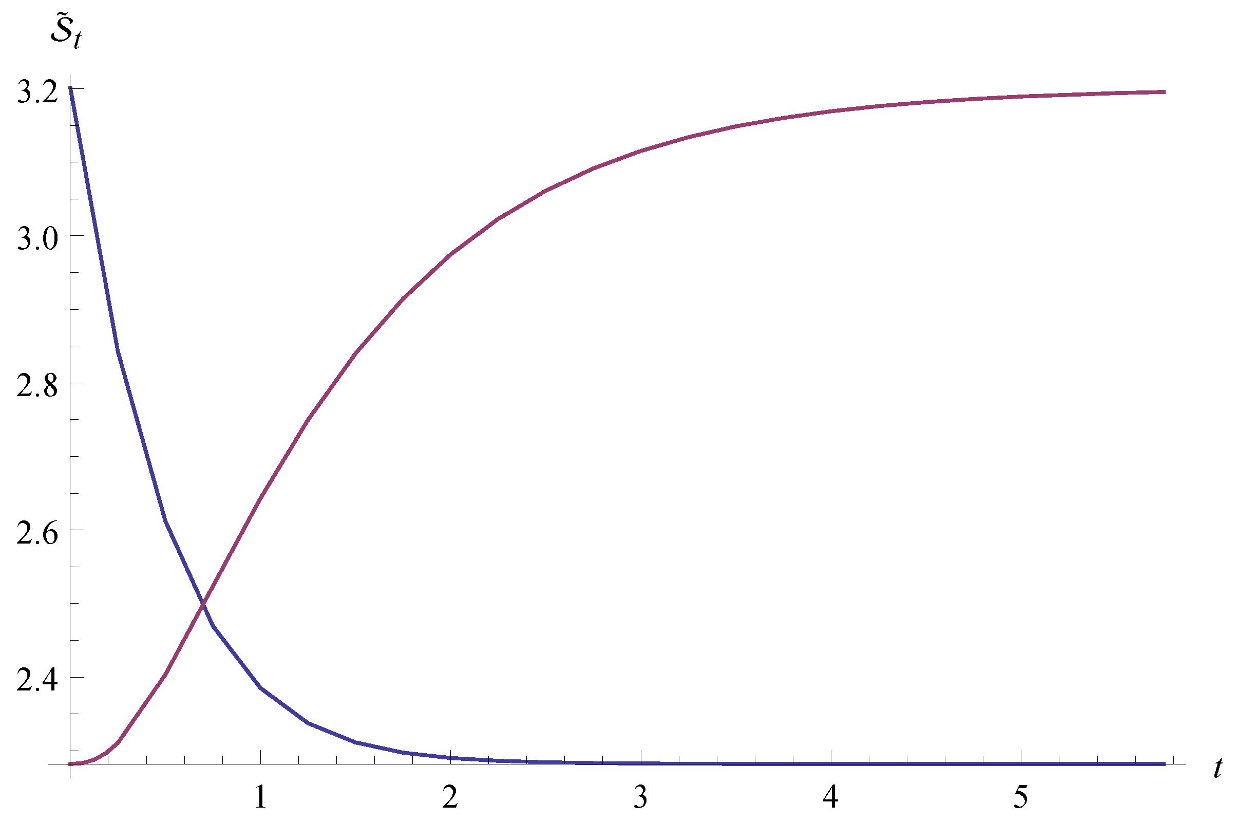
Figure 1.
Geometric entropy of the dynamical network model when the initial state is a fully-disconnected network (magenta line) and when it is a fully-connected network (blue line).
Figure 1.
Geometric entropy of the dynamical network model when the initial state is a fully-disconnected network (magenta line) and when it is a fully-connected network (blue line).
In
Figure 1, it is worth noting a crossing of the entropies’ time behaviors related to the two cases (links switched on and off). The first dynamics we dealt with switches on the links between nodes and shows how the entropy monotonically increases
vs. time. The maximum is asymptotically achieved and corresponds to the value computed for the fully-connected three-node network. The other dynamics considered describes a fully-connected network that switches off all of the links. In this case, the entropy monotonically decreases
vs. time. It asymptotically reaches the same value of that computed for the three-node networks with no links. Recall that the network dynamics is driven by the covariance matrices
given in (
31) and (
37). Then, at each time
t, we consider a set of local coordinates
, and the time dependent entropy (
28) is obtained as the logarithm of the volume of manifolds characterized by such a family (over
t) of coordinates. The dynamics is reflected into this quantity in a very expected way; indeed, as is shown in [
8], increasing or decreasing the topological dimension of the network, then the entropy increases or decreases, respectively. Therefore, adding links in the bare network amounts to growing the topological dimension up to the highest possible one represented by the fully-connected network. It is obvious that the contrary happens when the links are switched off from the fully-connected network.
Going further on, we consider intermediate situations with respect to the previous ones. That is, a network having initially one link and evolving in such a way that the other two links are switched on while the pre-existing one is switched off. This situation is characterized by, e.g.,
and:
Furthermore, we consider a network having initially two links and evolving in such a way the other link is switched on while the pre-existing switched off. This situation is characterized by, e.g.,
and:
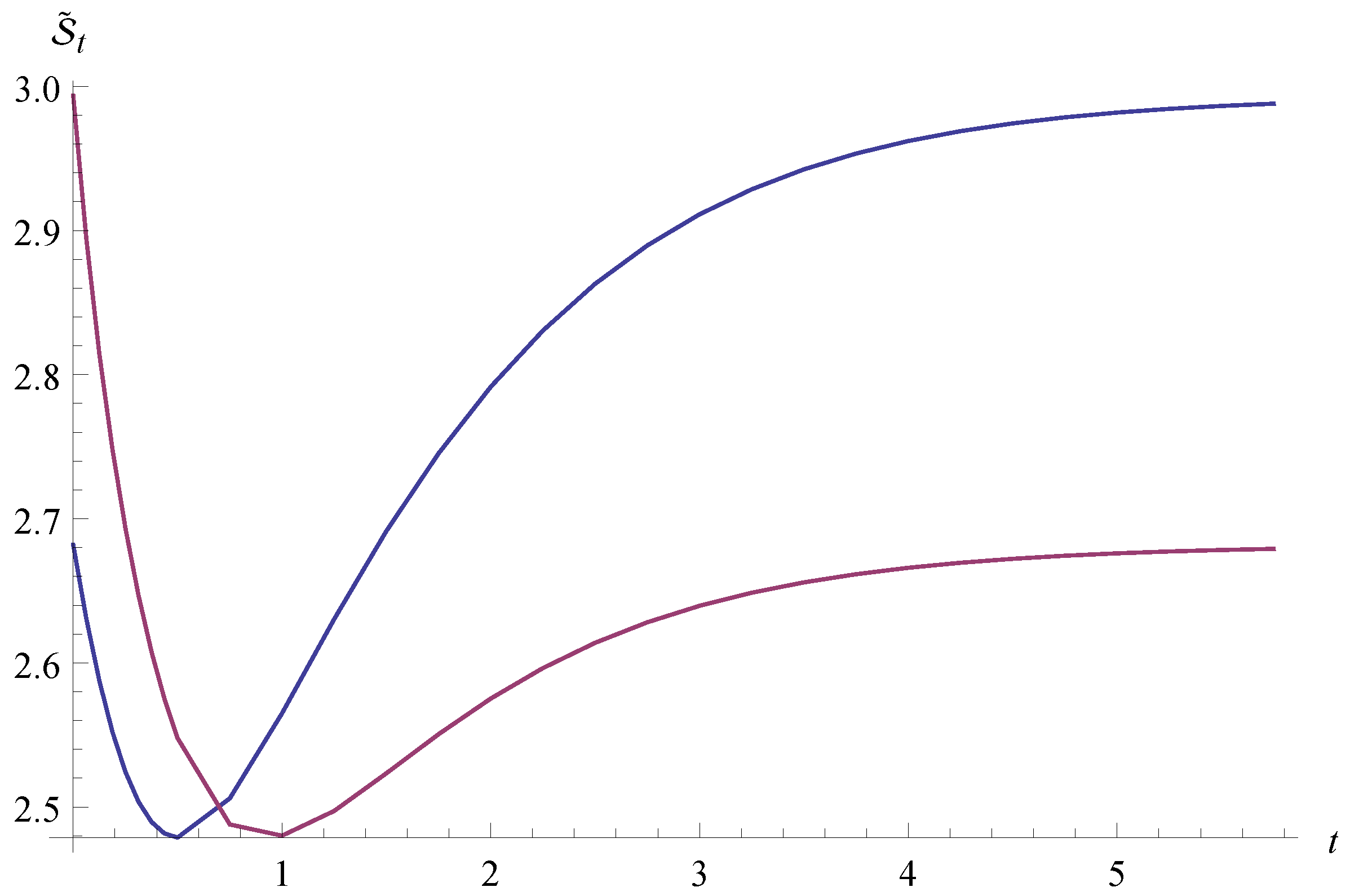
In these cases, the entropy shows a non-monotonic time behavior, as can be seen in
Figure 2. Actually, in both cases,
decreases towards a minimum and then rises up, reaching an asymptotic value. Each of these values corresponds to the initial value of the other curve. Here, the time-dependent entropy (
28) reflects a more complex behavior than the one in
Figure 1. Such a non-monotonic behavior could be explained by the fact that the dynamics described by Drifts (
41), (
43) involves two opposite processes, namely the switching on and off of links. Finally, it is worth highlighting that minimum values of the two curves are different; indeed, one is
(magenta line), while the other is
(red line).
Figure 2.
Geometric entropy of the dynamical network model when the initial state has two links (magenta line) and when it has one link (blue line).
Figure 2.
Geometric entropy of the dynamical network model when the initial state has two links (magenta line) and when it has one link (blue line).
5. Conclusions
In this work, we considered a way to associate a Riemannian manifold with a dynamical network interpreting random variables as sitting on vertices and their correlations as weighted links among vertices. We dealt with dynamics stemming from the Ornstein–Uhlenbeck process describing Gaussian networks’ evolution in order to account for switching on and off links. This entails dealing with a family
of Gaussian random variables. In such a way, we associated a Riemannian manifold with the network at each time
. It is worth remarking that at each time, a set of new local coordinates is provided. Hence, a mapping from
to
is supplied by the geometric entropy
of Equation (
28) in order to quantify the level of organization of the network along its time evolution.
Specifically, we considered a network with three vertices, and the dynamics is governed by Equation (
20) setting the drift matrix
to zero for every
and choosing the diffusion matrix
in order to describe the switching off and on of links.
The network’s evolution is reflected in the time behavior of the geometric entropy in a simple monotonic way when all links are switched on or off together. In contrast, the time behavior of the geometric entropy becomes more involved (with minima) when part of the links is switched on and part off. In any case, a crossing of the entropy time behaviors between switching on and off links occurs.
It is worth noticing the difference with time-dependent entropy of [
17] due to a network dynamics arising from an inference process [
13]. In the present work, we started from a definition of static entropy [
18] and then introduced a dynamics by the well-known Ornstein–Uhlenbeck process. In doing that, we considered a family of probability distributions and associate with it a network. Furthermore, the reverse process would be possible. In fact, given an
n-vertexes network, we can always consider associated with it
n random variables with correlations reflecting the edges disposition in the network and their weights. The problem is what kind of distribution do such variables have to respect. The choice could be done according to the type of network, or, better to say, to the kind of situation, or the system it represents. For instance, we may consider an electrical network where the edges are resistors and be interested in the voltage response on the current applied to each node. Then, voltages can be suitably described by a Gaussian probability distribution, which accounts for thermal noise (Johnson–Nyquist noise).
A natural extension of the present work would contemplate the same dynamics in larger networks where the interplay of various links and their (de)-synchronization could lead to a more complex time dependence of
. Additionally, it would be interesting to go beyond purely stochastic dynamics and see how deterministic components affect the geometric entropy. This could be done, for example, by including deterministic pairwise interactions and eventually self-dynamics of node variables too, similar to those considered in [
19].


