A Model for Scale-Free Networks: Application to Twitter

Abstract

In the last few years, complex networks have become an increasingly relevant research topic due to the large number of fields of application. Particularly, complex networks are especially significant in the area of modern online social networks (OSNs). OSNs are actually a challenge for complex network analysis, as they present some characteristics that hinder topology processing. Concretely, social networks’ volume is exceedingly big, as they have a high number of nodes and links. One of the most popular and influential OSNs is Twitter. In this paper, we present a model to describe the growth of scale-free networks. This model is applied to Twitter after checking that it can be considered a “scale-free” complex network fulfilling the small world property. Checking this property involves the calculation of the shortest path between any two nodes of the network. Given the difficulty of this computation for large networks, a new heuristic method is also proposed to find the upper bounds of the path lengths instead of computing the exact length.

1. Introduction

Online social networks (OSNs) are emerging as a new phenomenon in our communication society, powered by a virtually universal access to the Internet and the human need for socializing and sharing information. Thus, friends interchange information and organize common activities on Facebook or Tuenti; professionals keep in contact on LinkedIn; people from all walks of life communicate through short messages on Twitter, etc. There is a variety of forums, as well, where people interested in a given topic can post messages, chat, watch or download videos, share documents, pictures, slides, etc. The users of OSNs are not necessarily physical persons; the presence of institutions and corporations is increasing at a good pace. Interestingly, OSNs are also becoming an alternative to the conventional information channels, like newspapers and television.

Among OSNs, Twitter is one of the most popular. In a nutshell, Twitter can be described as a place for nanoblogging, where short messages or tweets (limited to 140 characters) posted by some members are read by their followers. Twitter has grown very rapidly over the past few years. Currently, Twitter has over 500 million users with 140 millions tweets posted daily and handles over 800,000 daily search requests, being one of the largest social networks of all time. Twitter came for the first time to newspapers’ front page in August 2011, because it was one of the communication channels used by street rioters in London. This fact prompted Scotland Yard to disrupt the communications on Twitter. Twitter played also a pivotal role in the Arab Spring [1] and in the Spanish 15M movement [2]. Therefore, it is really necessary to model this type of network to be able to predict future behaviors, to fight against malware and spam spreading, for marketing, etc.

Scale-free networks with a degree distribution following a power law have been the focus of a great deal of attention in the literature. This type of network characterizes the degree distributions of many man-made and naturally-occurring networks. For example, several types of social networks, including collaboration networks, appear to have a degree distribution with a power-law tail.

Many scale-free networks fulfill the small world property. This property consists of the fact that their average path length is very small compared to the size of the network. The computation of this property is very difficult for large networks, since it involves calculating the shortest path between any two nodes of the network. In this paper, a new heuristic method is proposed for proving this property for social networks.

Barabasi and Albert [3] have given the first explanation of the scale-free distribution by reformulating Simon’s model [4] in the context of growing networks. New nodes join the network by attaching m links to other nodes, chosen according to linear preferential attachment. This means that a node obtains one of the new links with a probability proportional to the number of links it already has. The algorithm, henceforth called the BA model, generates networks with a degree distribution $P\left(k\right)=2m^2{k}^{-3}$ with $k\ge m$. This model considers only undirected networks. Several variations and generalizations have been performed with this model for different authors to make a more realistic representation of processes taking place in real-world networks [5,6,7,8,9,10].

To model the growth of these social networks like Twitter, it is necessary to consider a more realistic perspective. Therefore, in this paper, a generalization of the BA model is proposed considering developing networks with directed links. In Section 2, an overview about complex networks is presented. In Section 3, it is verified that Twitter can be considered a complex network by surveying its topological structure. A new heuristic method to upper bound the path lengths is used to check the small world property. The data used in this study were taken in September 2009, thanks to the collaboration of Twitter administrators. The proposed model is introduced in Section 4. The application of this model to simulate Twitter’s growth is performed in Section 5. Finally, the conclusions obtained in this work are outlined in Section 6.

Our model simulates the topology and dynamics of the Twitter network. It can be further used as a starting point in simulating the information dynamics of the social network. There are many information-theoretic models that simulate the diffusion of messages [11,12,13,14,15,16]. They characterize the dynamics of retweeting activity, leading to interesting insights, such as users’ tweeting patterns in relation to their degree distribution or the ability to predict whether a piece of information will be virally transmitted through the network. As the next step in our work, tweeting activity can be assigned to our model’s nodes to implement the above-mentioned information propagation models. The goal would be to design a model able to successfully predict which information diffusion events will lead to bursts in network dynamics: whose tweets will be retweeted fastest and by the most nodes. The applications are obvious in simulating the diffusion of shocking news, spam messages, advertising and promotion campaigns, etc.

2. Complex Networks

In the field of network theory, a complex network is a graph whose topological structure shows some features that are not typical of simple networks, such as lattices or random graphs [17]. In recent years, the study of real-world networks has proven that, unlike what might be expected, many of them behave very differently from the standard Erdös–Rényi random graph model: the World Wide Web, Internet, movie actor collaboration networks, science collaboration graphs, the web of human sexual contacts, cellular networks, phone call networks, citation networks, networks in linguistics, power and neural networks, protein folding and many more [18].

Three concepts are of particular interest within the realm of complex networks, which are explained next.

• Degree distribution: In an undirected graph $G=(V,E)$, the degree of a node $v_i$ is the number of connections or edges that this node has to other nodes (excluding self-links), i.e.,

  $$deg{v}_i=\left|\{e_{ij}\in E:j\ne i\}\right|,$$

  where $\left|·\right|$ denotes cardinality. Furthermore, the degree distribution,

  $$P\left(k\right)=\frac{\left|\{v_i\in V:deg{v}_i=k\}\right|}{\left|E\right|},$$

  gives the fraction (or percentage) of nodes in V, the degree of which is $k\in \{0,1,...,n-1\}$, $n=\left|G\right|$. Therefore, $P\left(k\right)$ can be interpreted as the probability for a node (drawn randomly from V) of having exactly k edges.
  In Erdös–Rényi random networks, it has been shown [18] that $P\left(k\right)$ follows a Poisson distribution whose peak is located at $\langle k\rangle$ ($\langle ·\rangle$ denotes the expectation value). However, in many real-world networks, $P\left(k\right)$ follows a power-law distribution, that is,

  $$P\left(k\right)\sim k^{-\lambda }.$$

  (1)

  Networks with this property are called scale-free networks [19]. Equation (1) implies that scale-free networks have very few nodes that are highly connected, whereas the majority of them are not. Highly-connected nodes are called hubs, and their degrees tend to be orders of magnitude higher than that of the average nodes.
  Other functional dependencies on k are also found describing the degree distribution of real-world networks. Truncated power laws, exponential functions or Gaussian distributions are some examples of non-power laws that arise in many situations [20].
  In the case of directed graphs, there are in- and out-degrees (referring to incoming and outgoing edges, respectively) and the corresponding degree distributions. Needless to say, incoming and outgoing edges could follow different scaling laws.
• Clustering coefficient: This coefficient measures the tendency of a graph to form clusters of highly-related (i.e., connected) nodes, and it can be defined at a local and at a global level.
  For a particular node (local level), its clustering coefficient represents the degree of connection among its neighbors. The set of neighbors $N_i$ of a given node $v_i$ in a directed graph is defined as the set of nodes that are bidirectionally connected to $v_i$ (i.e., there is an edge from $v_i$ to the neighbor and also an edge from the same neighbor to $v_i$):

  $$N_i=\{v_j\in V:e_{ij}\in E,e_{ji}\in E\}.$$

  (2)

  The clustering coefficient $C_i$ of a node $v_i$ is then defined as the ratio of the number of links between the neighbors of $v_i$ to the maximum number of links possible,

  $$C_i=\frac{\left|\right\{e_{jk}\in E:v_j,v_k\in N_i\left\}\right|}{|N_i\left|\right(|N_i|-1)}.$$

  (3)

  Obviously, $C_i\in [0,1]$. At a global level, the clustering coefficient C of the whole network is computed as the mean value of all of the local clustering coefficients:

  $$C=\frac{1}{n}\sum _{i=1}^n{C}_i.$$

  (4)

  In random networks, which are meant to be undirected, the clustering coefficient depends on the probability of two random nodes being connected and can be easily computed from the mean degree $\langle k\rangle$ as [19]:

  $$C_{rand}=\frac{\langle k\rangle }{n}$$

  (5)

  According to Equation (5), random networks are expected to have a low clustering coefficient, since the mean degree $\langle k\rangle$ is usually low compared to the number of nodes of the network, n. Surprisingly, however, some real-world networks do have a clustering coefficient much larger than what is expected for a random network of the same size n. The fact is again evidence that real-world networks have an underlying structure considerably different from that of random ones.
• Average path length: This concept is defined as the average distance between any two nodes of the network, assuming that all nodes of the graph are connected to each other (i.e., for all $v_i,v_j\in V$, there is a sequence of nodes $\{v_i,v_{a_1},v_{a_2},\dots .v_{a_l},v_j\}$, called a path from $v_i$ to $v_j$ of length $l\ge 0$, such that $\{e_{i{a}_1},e_{a_1{a}_2},\dots ,e_{a_{l}j}\}\subset E$). Otherwise, one discards all isolated nodes; the result is (are) called the connected component(s) of the graph. The distance $d(v_i,v_j)$ from node $v_i$ to node $v_j$ in the same connected component is then the shortest distance of all paths joining $v_i$ to $v_j$. Note that, in the case of directed graphs, $d(v_i,v_j)\ne d(v_j,v_i)$ in general. The average path length $A_{length}$ is calculated according to:

  $$A_{length}=\frac{1}{n(n-1)}\sum _{i,j}d(v_i,v_j).$$

  (6)

  Depending on the convention used, Equation (6) may include paths from one node to itself (so-called cycles), but in practice, this possibility barely affects the results.
  Real-world networks usually fall into the category of small world networks. Small world networks are characterized by the fact that their average path length is very small compared to the size of the network. This interesting property is not so uncommon though, since it can also be found in random networks [21].

Over the past several years, many studies have been carried out to analyze the complex topological structure of several real-world networks. The World Wide Web is such an example: web pages form the set of nodes of the network, and the hyperlinks among them are the edges. Despite the large number of web pages on the Internet and the links among them, its structure shows a very low average path length, a high clustering coefficient and a power-law-based degree distribution. Other examples of artificial networks with a special topological structure include the Internet (composed of routers and their connections to computers), power networks (the grid of the western United States), scientific collaboration networks and several biologically-based networks. For a detailed list of examples where complex connectivities were observed emerging from real-world networks, see [18].

3. Twitter as a Complex Network

The Twitter network consists of users and their relationships, so it can be naturally modeled as a directed graph $G=(V,E)$, where:

• $V=\{v_1,v_2,\dots ,v_n\}$ is the set of nodes (or vertices) of the graph. Here, each $v_i$ represents a Twitter user, and n is the number of users. By definition, the number of nodes is the cardinality of the graph (in symbols: $n=\left|G\right|$).
• E is the set of directed edges (or links). An edge $e_{ij}$ is an ordered pair of nodes of the form $(v_i,v_j)$, meaning that the edge goes from $v_i$ to $v_j$. If there exists a relationship between two users $v_i$ and $v_j$ in the sense that $v_i$ follows $v_j$ (in Twitter terms), then there is a corresponding edge $e_{ij}=(v_i,v_j)\in E$ in the Twitter graph.

Equivalently, one says that $v_i$ is a follower of $v_j$ or that $v_j$ is a friend of $v_i$. Although, in general graphs, there can be edges of the form $e_{ii}$ (i.e., from node $v_i$ to itself), this is not the case in the graph representing Twitter.

3.1. Data Gathering

As was mentioned in the Introduction, Twitter has currently some 500 million users, and counting. Therefore, gathering the data required to analyze Twitter’s topological structure poses a difficult problem. The Twitter public API [22] is the standard tool used by many web applications to retrieve data from Twitter users’ accounts and to compute useful statistics, such as social influence metrics (see, for instance, Klout [23] and Twitalyzer [24]). However, Twitter imposes a restriction on all users accessing the API, in such a way that only 350 queries can be performed per hour, which in effect makes it impossible to collect the necessary information to build a snapshot of the Twitter network at a certain time. Fortunately, in [25], the authors were able to obtain such a snapshot (Twitter administrators kindly removed the access limit for them), which was then made publicly available.

The dataset that was finally used for this study contains social data from 50 million users. The snapshot was taken in September 2009 and contains $1,963,263,821$ friendship links among $51,217,936$ users.

3.2. Degree Distribution

The degree distribution of many real-world networks is not Poissonian, showing that they have not much in common with the classical random network model. For instance, the degree distribution of the Internet is accurately modeled by a power law [26]. However, in some cases, such as the collaboration network between scientists (two scientists are connected if they have coauthored a paper), it can be better represented by a truncated power law (i.e., $P\left(k\right)\sim k^{-\lambda }{e}^{-k/k_c}$) [27]. Other networks show a completely different degree distribution, such as the power grid of the western United States, which follows an exponential distribution, or the Utah Mormon social network, which shows a Gaussian distribution [20].

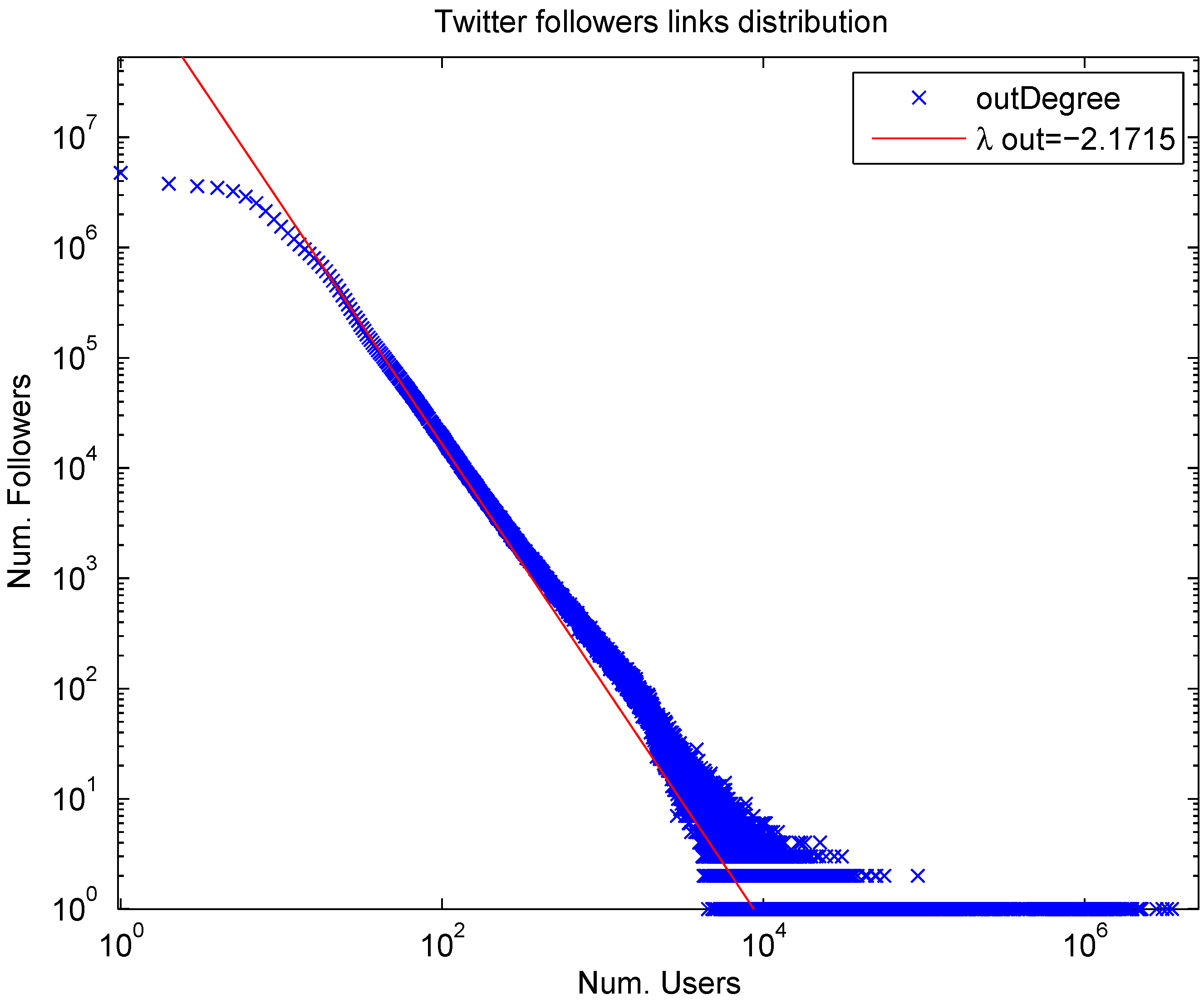
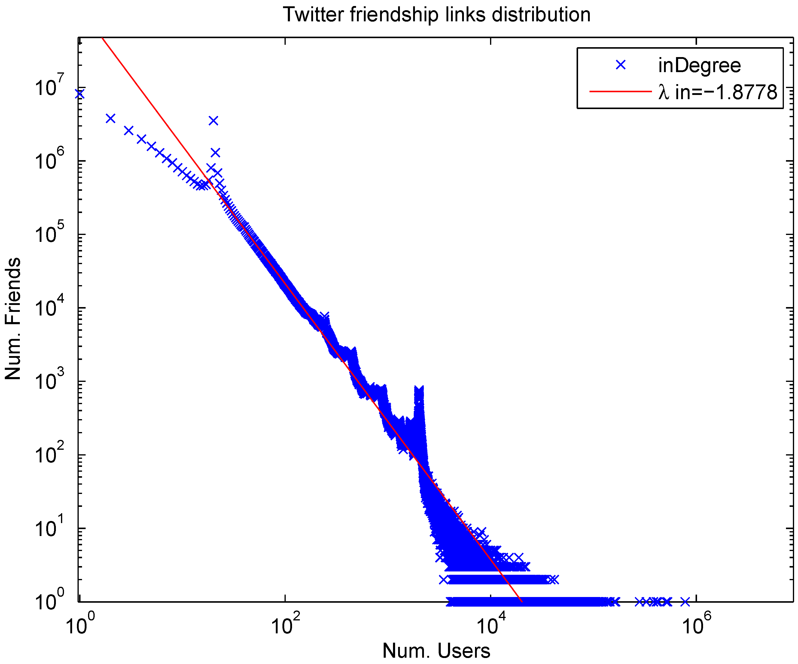
Since Twitter is a directed network, two degree distributions can be actually studied: (i) the outgoing degree distribution $P_o\left(k\right)$ (relative frequency of nodes with k outgoing edges); and (ii) the incoming degree distribution $P_i\left(k\right)$ (relative frequency of nodes with k incoming edges). Figure 1 and Figure 2 show $P_o\left(k\right)$ and $P_i\left(k\right)$ of Twitter, respectively. Both figures have been plotted in logarithmic scale. As one can see, they nicely resemble straight lines, showing that both degree distributions follow approximately a power law. As a result, Twitter is characterized by the presence of “friend” and “follower” hubs.In other words, there are few users with a large group of followers, as well as few users with a large group of friends, while the majority of users have a few friends and followers.

Twitter can therefore be categorized as a scale-free network. How scale-free networks come about can be explained by growth based on preferential attachment [3]. According to this assumption, as the network grows, new nodes are more likely to connect to high degree nodes than to low degree nodes. This is also known as “the rich gets richer” philosophy and is observed in the Twitter network, since new users tend to follow important (i.e., highly connected) users.

Figure 1. Outgoing degree distribution of Twitter’s network. As the figure shows, there are a few users with an enormous degree (number of friends). On the contrary, the majority of them have just at most 1000 friends.

Figure 1. Outgoing degree distribution of Twitter’s network. As the figure shows, there are a few users with an enormous degree (number of friends). On the contrary, the majority of them have just at most 1000 friends.

Figure 2. Incoming degree distribution of Twitter’s network. As the figure shows, there are a few users with an enormous degree (number of followers). On the contrary, the majority of them have less than 100 followers.

Figure 2. Incoming degree distribution of Twitter’s network. As the figure shows, there are a few users with an enormous degree (number of followers). On the contrary, the majority of them have less than 100 followers.

3.3. Clustering Coefficient

As explained in Section 2, the clustering coefficient of a node measures how much connected it is to its neighbors. The clustering coefficient of a node in a directed graph is given by Equations (2) and (3), and the clustering coefficient for the whole network is obtained from Equation (4).

The expected clustering coefficient in random networks is computed via Equation (5). In random networks, the mean degree $\langle k\rangle$ is usually orders of magnitude lower than the number of nodes n, so the clustering coefficient tends to be a small value.

Many real-world networks, however, have a much higher clustering coefficient than what is expected according to the random network model. For a random network of the same size as that of Twitter’s network, the expected clustering coefficient is, according to Equation (5),

$$C_{Twitter\_rand}=\frac{\langle k\rangle }{n}=\frac{38.33}{51.22\times {10}^6}=7.48\times {10}^{-7},$$

where the mean node degree $\langle k\rangle$ was obtained by dividing the number of links ($1963\times {10}^6$) by the number of nodes ($51.22\times {10}^6$). However, Twitter is a directed network, thus $C_{Twitter\_rand}$ must be divided by two, resulting in $3.74\times {10}^{-7}$. The analysis of the actual Twitter network provides quite different results though (see Table 1).

Table 1. Twitter network clustering coefficient.

Random network C. Coef.	Twitter network actual C. Coef.	Ratio
$3.74\times {10}^{-7}$	$0.096$$(9.6\%)$	$256,684.5$

Table 1. Twitter network clustering coefficient.

Random network C. Coef.	Twitter network actual C. Coef.	Ratio
$3.74\times {10}^{-7}$	$0.096$$(9.6\%)$	$256,684.5$

The results of Table 1 show that the Twitter clustering coefficient is much larger than that of a random network of the same size (specifically, it is almost ${10}^5$-times larger). We conclude that Twitter users tend to form clusters according to friendship links.

3.4. Average Path Length

Whether a network may be called a small world network depends on the average path length, which must be very short compared to the size of the network. Many real-world networks fall into this category, but so do random networks, as well.

Computing the average path length is a difficult task, since it involves calculating the shortest path between any two nodes of the network. Traditionally, algorithms, such as Floyd-Warshall’s [28] or Johnson’s [29], have been used for computing the distance between all pairs of nodes in a graph. Unfortunately, as the size of the graph grows larger, their execution time rapidly increases, rendering them useless for graphs, such as the Twitter network model. Specifically, the Twitter network is composed of $51,217,936$ users; $43,027,729$ of them have at least one friend (i.e., they are the beginning of a link), and $48,192,718$ of them have at least one follower (i.e., they are the end of a link). Therefore, there are $43,027,729\times 48,192,718\approx$ $2073\times {10}^{12}$ potential paths, making the brute force approach infeasible. To overcome this problem, a new method is proposed to prove the small world property for Twitter’s network. Instead of computing the exact length of all of the paths, we will content ourselves with upper bounds of the path lengths and average path length. Note that a small upper bound of the path lengths means that all paths are at most as long, but not any longer. As a consequence, finding a small upper bound of the path lengths would prove that all of the paths are short enough to make Twitter a small world network.

3.4.1. Method

The new method presented here for estimating an upper bound of the average path length is mainly based on the existence of hubs. The idea behind it is very simple. Consider for a moment a undirected graph with several hubs. Since hubs are connected to a large amount of nodes, they are an easy way to quickly go from one node to another. For instance, if a path from $v_i$ to $v_j$ must be found and $h_k$ is a hub, then it is very likely that $h_k$ is connected to both $v_i$ and $v_j$, leading to the short path $\{v_i,h_k,v_j\}$. Since, however, the graph we have associated with the Twitter network is directional, only nodes with a large number of both outgoing and incoming links will be promoted to hubs.

Our method, inspired by the idea presented above, makes the problem computationally amenable by introducing a strongly-connected component, called the hub subnetwork and denoted by $G_h=(V_h,E_h)$, $V_h=\{h_1,...,h_{\left|V_h\right|}\}$. This hub subnetwork consists of nodes with both many friends (outgoing links) and followers (incoming links), so virtually any pair of nodes can be connected through it. The method is divided into three stages.

• For every node that is not in the hub subnetwork, find one path from it to any hub. Call $d(v_i,V_h)$ its length, $〈d(v_i,V_h)〉$ the average of all distances $d(v_i,V_h)$ and ${max}_{toHub}={max}_{v_i\notin V_h}d(v_i,V_h)$ their maximum.
• For every hub, find one path to any other hub. Call $d(h_i,h_j)$ its distance, $〈d(h_i,h_j)〉$ the average of all distances $d(h_i,h_j)$ and ${max}_{withinHub}={max}_{h_i,h_j\in V_h}d(h_i,h_j)$ their maximum.
• For every node that is not in the hub subnetwork, find one path from any hub to that node. Call $d(V_h,v_i)$ its length, $〈d(V_h,v_i)〉$ the average of all distances $d(V_h,v_i)$ and ${max}_{fromHub}={max}_{v_i\notin V_h}d(V_h,v_i)$ their maximum.

Figure 3 depicts this approach. Then:

$${\text{max}}_{length}={\text{max}}_{toHub}+{\text{max}}_{withinHub}+{\text{max}}_{fromHub}$$

(7)

is an upper bound of the distance from any node of the network to any other, and:

$$〈d〉=〈d(v_i,V_h)〉+〈d(h_i,h_j)〉+〈d(V_h,v_i)〉$$

(8)

is an upper bound of the mean distance of the Twitter network.

Nevertheless, this approach makes some assumptions that might not hold:

• It is always possible to find a path from any node to the hub subnetwork.
• There is a path between any two nodes within the hub subnetwork.
• It is always possible to go from any node of the hub subnetwork to any other node in the graph.

Figure 3. Three-stage methodology for computing the path between two nodes.

Figure 3. Three-stage methodology for computing the path between two nodes.

Fortunately, by carefully selecting the nodes of the hub subnetwork, these three assumptions may be considered as good as true (see below for details). Indeed, the high in- and out-connectivity of the hub nodes makes it easy to find paths from any node of the network to the hub network, as well as from the hub network to any other node. The selection process produced a hub subnetwork with 1000 nodes, these being the users with the most friends that also happened to have a large group of followers. On average, each hub has $47,351$ friends and $67,622$ followers.

In order to compute ${max}_{toHub}$, it is necessary to find a path from any node outside the hub subnetwork to the hub subnetwork. To this end, a breadth-first search starting from each such node is performed. Each search stops when any hub is reached. ${max}_{toHub}$ is then the maximum length of all of the found paths. By construction, ${max}_{toHub}$ is certainly an upper bound of the greatest distance from any node to the hub subnetwork.

The parameter ${max}_{withinHub}$ can be easily computed by exhaustive searching, since only $1000\times 1000$ paths must be found. After finding all distances between pairs of hubs, ${max}_{withinHub}$ is set to be the maximum distance.

Obtaining ${max}_{fromHubs}$ can be more complicated than ${max}_{toHub}$, if one tries to find paths from the hubs to any other node that is not in the hub subnetwork. The reason is that finding a path from a simple node to a hub is easier than the other way around. To circumvent this difficulty, an auxiliary network was created solely for this purpose, this new network being identical to the original Twitter network, but with inverted links. Therefore, an edge from $v_i$ to $v_j$ means in the auxiliary network that user $v_j$ is a follower of $v_i$. Clearly, its ${max}_{toHub}$ value matches the ${max}_{fromHub}$ value of the original Twitter network, so the same method explained above for computing ${max}_{toHub}$ can be used.

3.4.2. Results

The relevant parameter values are provided below using the new proposed method to estimate the average path length of the dataset used for this study.

• $ma{x}_{toHub}$
  The maximum length of all of the paths found between any node and the hub subnetwork is:

  $${max}_{toHub}=45.$$

  However, the average path length is much lower,

  $$〈d(v_i,V_h)〉=1.79.$$
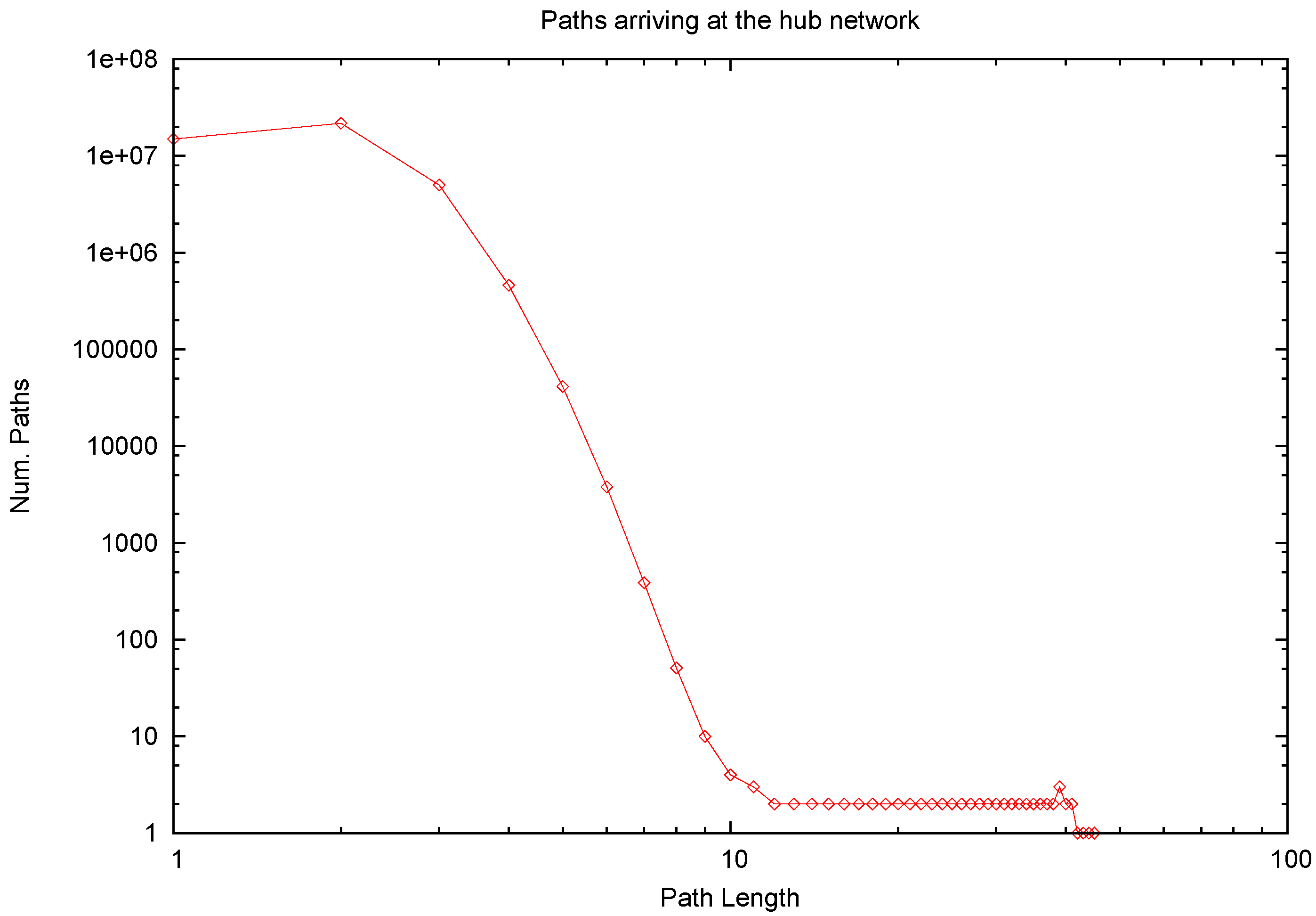
  The distribution of path lengths is shown in Figure 4, where it can be checked that most of them have a length of three or less. Moreover, a total amount of $42,213,921$ paths (each with a different initial node) was found. Taking into account the fact that there are $43,027,729$ users with at least one friend, this means that in $98.10\%$ of the cases, the search of a path from a node outside the hub subnetwork to a hub was successful.

  No. of Paths	Path Length
  …	…
  10	9
  51	8
  387	7
  3,789	6
  41,337	5
  461,414	4
  4,998,876	3
  21,755,660	2
  14,951,325	1
  1,000	0

  Figure 4. Path length distributions ending at a node of the hub network. The few paths with a length greater than or equal to 10 have been omitted in the table.

  Figure 4. Path length distributions ending at a node of the hub network. The few paths with a length greater than or equal to 10 have been omitted in the table.
• $ma{x}_{withinHub}$
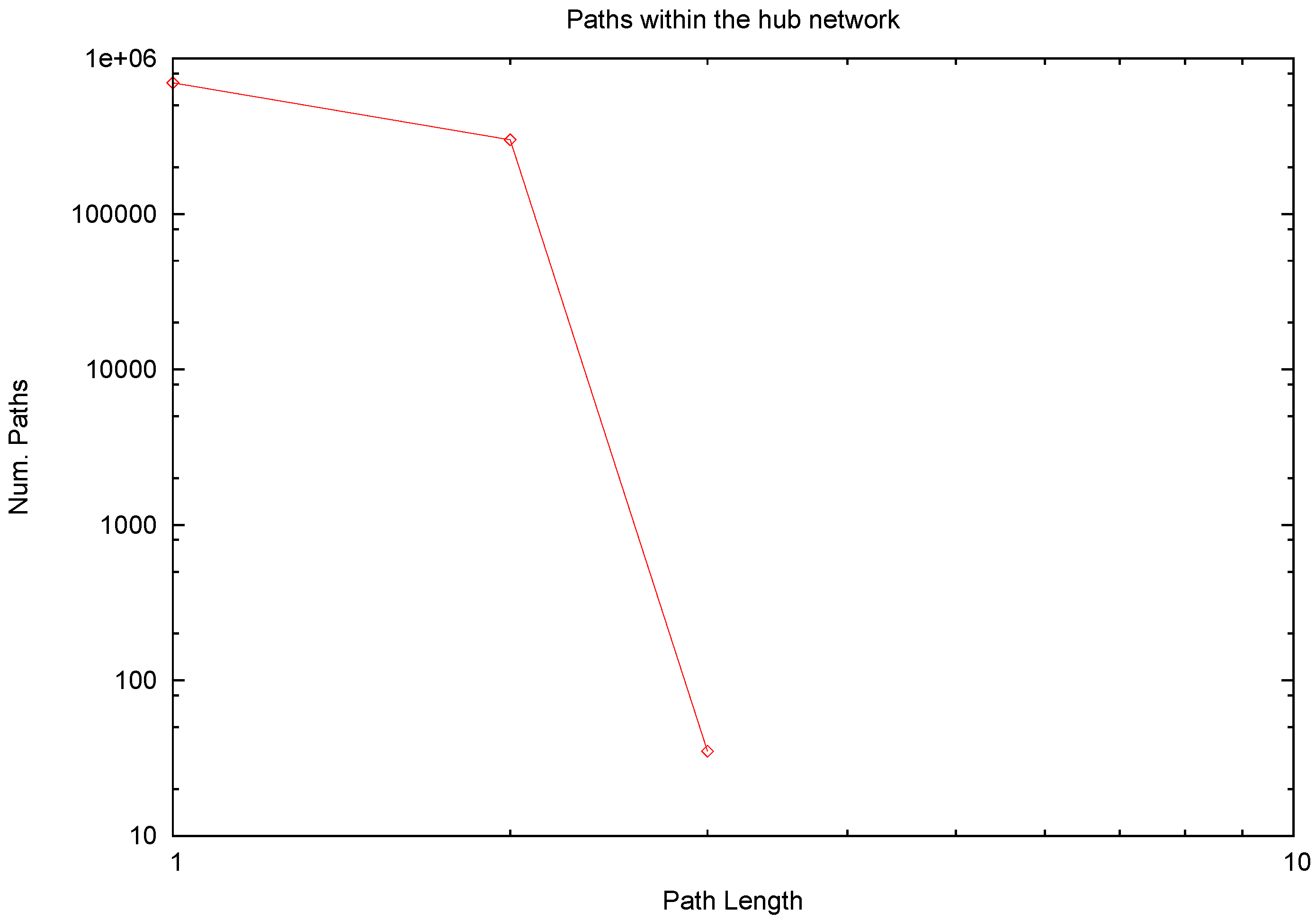
  The maximum length of all of the paths found from one hub to another is:

  $${\text{max}}_{withinHub}=3,$$

  and their average,

  $$〈d(h_i,h_j)〉=1.30.$$
  Figure 5 shows the distribution of path lengths in the hub subnetwork.

  No. of Paths	Path Length
  35	3
  299,884	2
  699,081	1
  1,000	0

  Figure 5. Path length distributions within the hub subnetwork.

  Figure 5. Path length distributions within the hub subnetwork.
• $ma{x}_{fromHub}$
  The maximum length of all of the paths found from the hub subnetwork to any other node is:

  $${max}_{fromHub}=12.$$

  However, as in the case of ${max}_{toHub}$, the average path length is much lower, namely,

  $$〈d(V_h,v_i)〉=2.19.$$
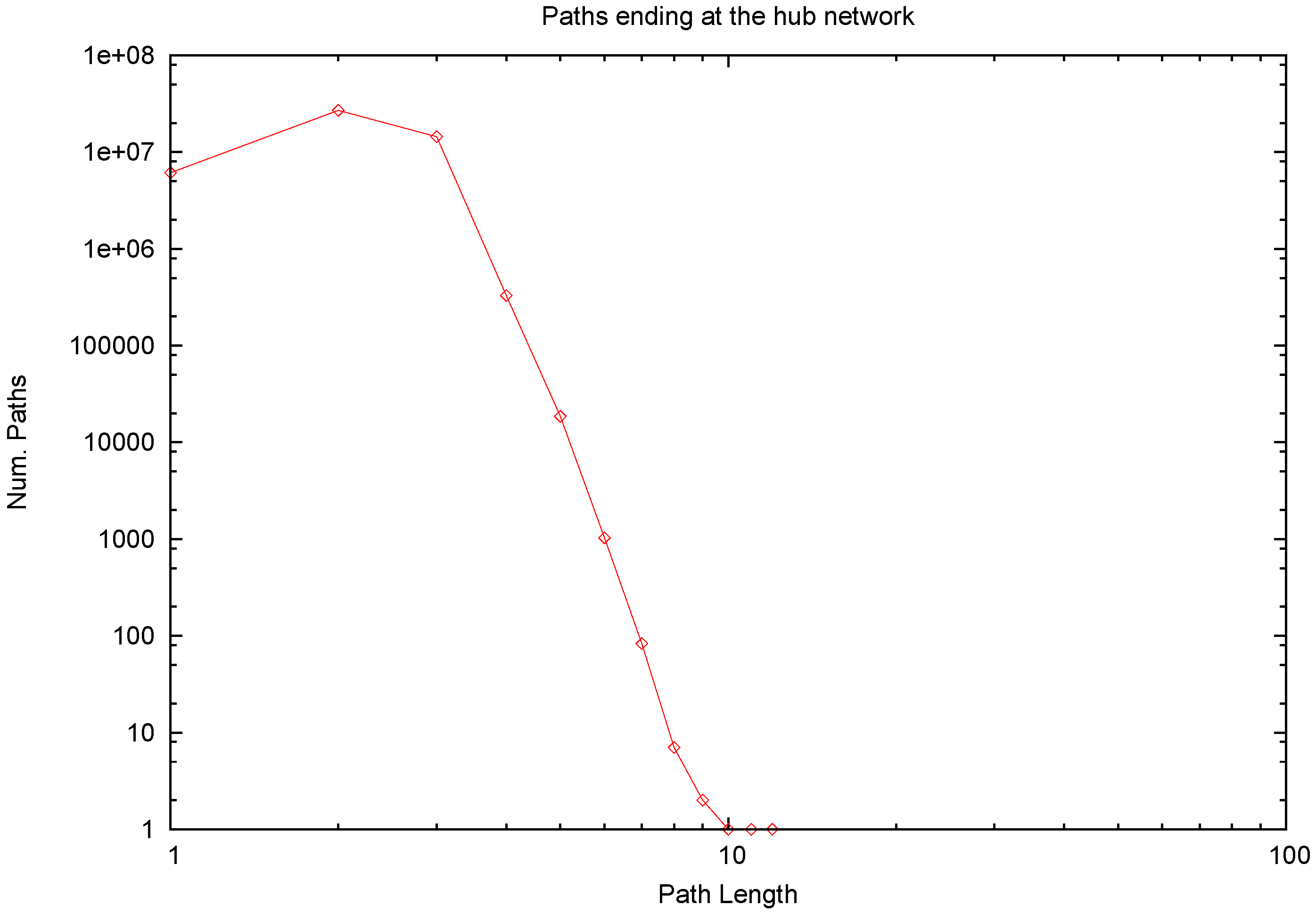
  The distribution of path lengths is shown in Figure 6, where it can be seen that most of them have a length of three or less. Moreover, the total count of paths (each with a different initial node) was $48,044,814$. Taking into account that there are $48,192,718$ users with at least one follower, this means that in $99.69\%$ of the cases, the search of a path from the hub subnetwork to a node outside was successful.

  No. of Paths	Path Length
  1	12
  1	11
  1	10
  2	9
  7	8
  83	7
  1,033	6
  18,578	5
  330,156	4
  14,467,363	3
  27,089,900	2
  6,136,689	1
  1,000	0

  Figure 6. Path length distributions starting from the hub network.

  Figure 6. Path length distributions starting from the hub network.

3.4.3. Resulting Upper Bounds

From the previous data, and Equations (7) and (8), it follows that:

$${max}_{length}=45+3+12=60,$$

(9)

and:

$$〈d〉=1.79+1.30+2.19=5.28.$$

(10)

Having made the simple math, a final remark is in order.

As mentioned above, the hub subnetwork was reached by $42,213,921$ nodes, and $48,044,814$ nodes could be reached from the hub network. This means that the total amount of paths included in the calculations is $42,213,921\times 48,044,814=2028\times {10}^{12}$ out of the $43,027,729\times 48,192,718=2073\times {10}^{12}$ potential paths (once the isolated nodes of Twitter’s network have been removed), provided there is a path between any pair of nodes. Therefore, the sample used for the calculation of ${max}_{toHub}$ and $〈d〉$ might cover even more than $97.83\%$ of the actual paths (one per pair of nodes), just obtained after dividing those numbers. Our sample being practically exhaustive, we may conclude that the results Equations (9) and (10) are not only conservative, but also statistically significant.

4. The Model

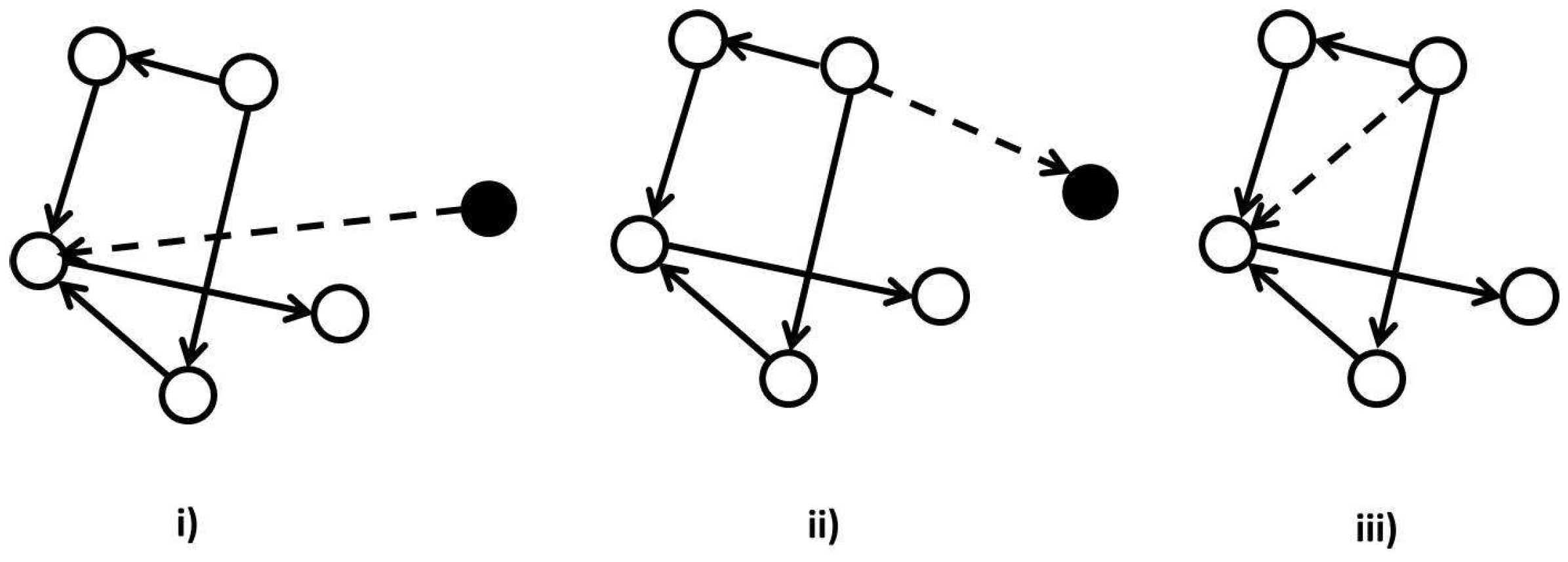
In social networks, every instant, new nodes and links are created while some others are removed. In this paper, we propose a model based on developing networks with directed links that show a scaling behavior, but we did not contemplate the decaying behavior to avoid complicating the model. We consider structures that evolve due to the following reasons. First, they grow as in the BA model, i.e., in each instant, one new node is added and is connected to an old node by a directed link with a probability depending only on the in- or out-degree of the target. If the new node is attached to the old node Figure 7 i), the probability depends only on the in-degree, and if it is attached as the target of the old node Figure 7 ii), the probability depends on the out-degree of the target. In addition, we introduce a new parallel component of the evolution Figure 7 iii): the permanent addition of new directed links between old nodes depending on the out-degree of the target and the in-degree of the originating node. In this section, we follow the same notation as in [10].

Figure 7. Growth process in the model: (i) node creation attaching an old node; (ii) node creation as the target of an old node; (iii) link creation. In (i) and (ii), the new node is a filled black circle, while in (i), (ii) and (iii), the new link is a dashed line.

Figure 7. Growth process in the model: (i) node creation attaching an old node; (ii) node creation as the target of an old node; (iii) link creation. In (i) and (ii), the new node is a filled black circle, while in (i), (ii) and (iii), the new link is a dashed line.

Let us first determine the average node degrees (in-degree, out-degree and total degree) of the model. Let $N\left(t\right)$ be the total number of nodes and $I\left(t\right)$ and $J\left(t\right)$ the in-degree and out-degree of the entire network, respectively. At each time step,

• with probability p, a new node is created attaching to a directed node,
• with probability q, a new node is created attached by a directed link and
• with probability r, a directed link is created between the old nodes.

The probabilities p, q and r should clearly add up to unity, and we always assume $q<p$. Therefore, both the total in- and out-degrees increase by one. As a result, $N\left(t\right)=(p+q)t$ and $I\left(t\right)=J\left(t\right)=t$ and the average in- and out-degrees, ${\mathfrak{D}}_{in}=I\left(t\right)/N\left(t\right)$ and ${\mathfrak{D}}_{out}=J\left(t\right)/N\left(t\right)$, are both equal to $\frac{1}{p+q}$.

To determine the degree distributions, we need to specify:

• (i) the attachment rate $A(i,j)$, defined as the probability that a newly-introduced node links to an existing node with i incoming and j outgoing links,
• (ii) the attachment rate $B(i,j)$, defined as the probability that a newly-introduced node is linked by an existing node with i incoming and j outgoing links,
• (ii) the creation rate $C(i_1,j_1|i_2,j_2)$, defined as the probability of adding a new link from a $(i_1,j_1)$ node to a $(i_2,j_2)$ node.

We consider that the attachment rate $A(i,j)$ depends only on the in-degree of the target node and that the attachment rate $B(i,j)$ depends only on the out-degree of the source node; therefore, $A(i,j)=A_i=i+\lambda$ and $B(i,j)=B_j=j+\nu$, where λ and ν are constants. In the same spirit, we take the link creation rate to depend only on the out-degree of the issuing node and the in-degree of the target node, $C(i_1,j_1|i_2,j_2)=C(j_1,i_2)=(i_2+\lambda )(j_1+\nu )$.

With these rates, the joint degree distribution, $N_{ij}\left(t\right)$, defined as the average number of nodes with i incoming and j outgoing links, evolves according to:

$$\begin{array}{cc}\hfill \frac{d{N}_{ij}\left(t\right)}{dt}=& (p+r)\left[\frac{(i-1+\lambda )N_{i-1,j}-(i+\lambda )N_{ij}}{I+\lambda N}\right]+\hfill \\ & (q+r)\left[\frac{(j-1+\nu )N_{i,j-1}-(j+\nu )N_{ij}}{J+\nu N}\right]+p{\delta }_{i0}{\delta }_{j1}+q{\delta }_{i1}{\delta }_{j0}.\hfill \end{array}$$

(11)

The first group of terms on the right accounts for the changes in the in-degree of target nodes by simultaneous creation of a new node and link (probability p) or by creation of a new link only (probability r). For example, the creation of a link to a node with in-degree i leads to a loss in the number of such nodes. This occurs with rate $(p+r)(i+\lambda )N_{ij}$, divided by the appropriate normalization factor ${\sum }_{i,j}(i+\lambda )N_{ij}=I+\lambda N$. Similarly, the second group of terms account for out-degree changes. The third term accounts for the introduction of new nodes with no incoming links and one outgoing link. The last term appears for the introduction of new nodes with one incoming link and no outgoing links.

It is clear that the $N_{ij}$ grow linearly with time. Accordingly, we substitute $N_{ij}\left(t\right)=t{n}_{ij}$, as well as $N=(p+q)t$, $I=J=t$ and $r=1-p-q$, into Equation (11) to yield a recursion relation for $n_{ij}$:

$$\begin{array}{c}\left[(1+\lambda (p+q\left)\right)+(1-q)(i+\lambda )+(1-p)(j+\nu )\right]n_{ij}=\hfill \\ (1-q)(i-1+\lambda )n_{i-1,j}+(1-p)(j-1+\nu )n_{i,j-1}+\\ \hfill p\left[1+\lambda (p+q)\right]{\delta }_{i0}{\delta }_{j1}+q\left[1+\lambda (p+q)\right]{\delta }_{i1}{\delta }_{j0}.\end{array}$$

(12)

The in-degree and out-degree distributions are straightforwardly expressed through the joint distribution: ${\mathcal{I}}_i\left(t\right)={\sum }_j{N}_{ij}\left(t\right)$ and ${\mathcal{O}}_j\left(t\right)={\sum }_i{N}_{ij}\left(t\right)$. Because of the linear time dependence of the node degrees, we write ${\mathcal{I}}_i\left(t\right)=t{I}_i$ and ${\mathcal{O}}_j\left(t\right)=t{O}_j$. The densities $I_i$ and $O_j$ satisfy:

$$\begin{array}{c}\left[(1+(1-q)i+\lambda (1+p)\right]I_i=\hfill \\ \hfill (1-q)(i-1+\lambda )I_{i-1}+p\left[1+\lambda (p+q)\right]{\delta }_{i0}+q\left[1+\lambda (p+q)\right]{\delta }_{i1}\end{array}$$

(13)

and:

$$\begin{array}{c}\left[(1+\lambda (p+q\left)\right)+(1-p)(j+\nu )\right]O_j=\hfill \\ \hfill (1-p)(j-1+\nu )O_{j-1}+p\left[1+\lambda (p+q)\right]{\delta }_{j1}+q\left[1+\lambda (p+q)\right]{\delta }_{j0},\end{array}$$

(14)

respectively. The solution to these recursion formulae may be expressed in terms of the following ratios of gamma functions:

$$I_i=\frac{\Gamma (i+\lambda )\Gamma (\frac{2+\lambda (1+p)-q}{1-q}+1)}{\Gamma (i+\frac{\lambda (1+p)+1}{1-q}+1)\Gamma (1+\lambda )}{I}_1,\text{for}i\ge 1$$

(15)

with $I_0=\frac{p\left[1+\lambda (p+q)\right]}{1+\lambda (1+p)}$, $I_1=\frac{\lambda (p+q)\left[1+\lambda (p+q)\right]+q}{\left[1+\lambda (1+p)\right]\left[2-q+\lambda (1+p)\right]}$ and:

$$O_j=\frac{\Gamma (j+\nu )\Gamma (\frac{2+\nu (1+q)-p}{1-p}+1)}{\Gamma (j+\frac{\nu (1+q)+1}{1-p}+1)\Gamma (1+\nu )}{O}_1,\text{for}j\ge 1$$

(16)

with $O_0=\frac{q\left[1+\nu (p+q)\right]}{1+\nu (1+q)}$, $O_1=\frac{\nu (p+q)\left[1+\nu (p+q)\right]+p}{\left[1+\nu (1+q)\right]\left[2-p+\nu (1+q)\right]}.$

From Equations (15) and (16), we see that as $i,j\to \infty$, we have $I_i\sim C_{IN}{i}^{-{\lambda }_{IN}}$ and $O_j\sim C_{OUT}{j}^{-{\lambda }_{OUT}}$, respectively, with:

$${\lambda }_{IN}=\frac{1+\lambda (p+q)}{1-q}+1\text{and}{\lambda }_{OUT}=\frac{1+\nu (p+q)}{1-p}+1.$$

(17)

Therefore, in this section, a generalization of the BA model is proposed to describe the behavior of social networks. The BA model only considers undirected networks, and every instant, a new node is created linked to the network node with the highest degree. This model offers a more realistic point of view considering directed networks, and the creation of new nodes attaching or attached to a node and new links between old nodes depending on their in- and out-degree. It would be very interesting to add the decaying network behavior of social networks. This behavior consists of removing links or nodes with a lower probability than the creation of new ones. This property makes the model too complicated and difficult to find a mathematical representation.

Our model can be used to simulate “scale-free” networks and to study different parameters about how information is spread considering the selected application.

5. Application of the Model to Twitter

In this section, the model proposed in Section 4 is applied to Twitter. From Section 3, we know the power law values ${\lambda }_{IN}=2.2$ and ${\lambda }_{OUT}=1.9$ and the average in- and out-degrees ${\mathfrak{D}}_{in}={\mathfrak{D}}_{out}=38.33$. Substituting these values in Equation (17), the following expressions are obtained:

$$0.2-1.2q=0.026\lambda \text{and}-0.123+0.9q=0.026\nu .$$

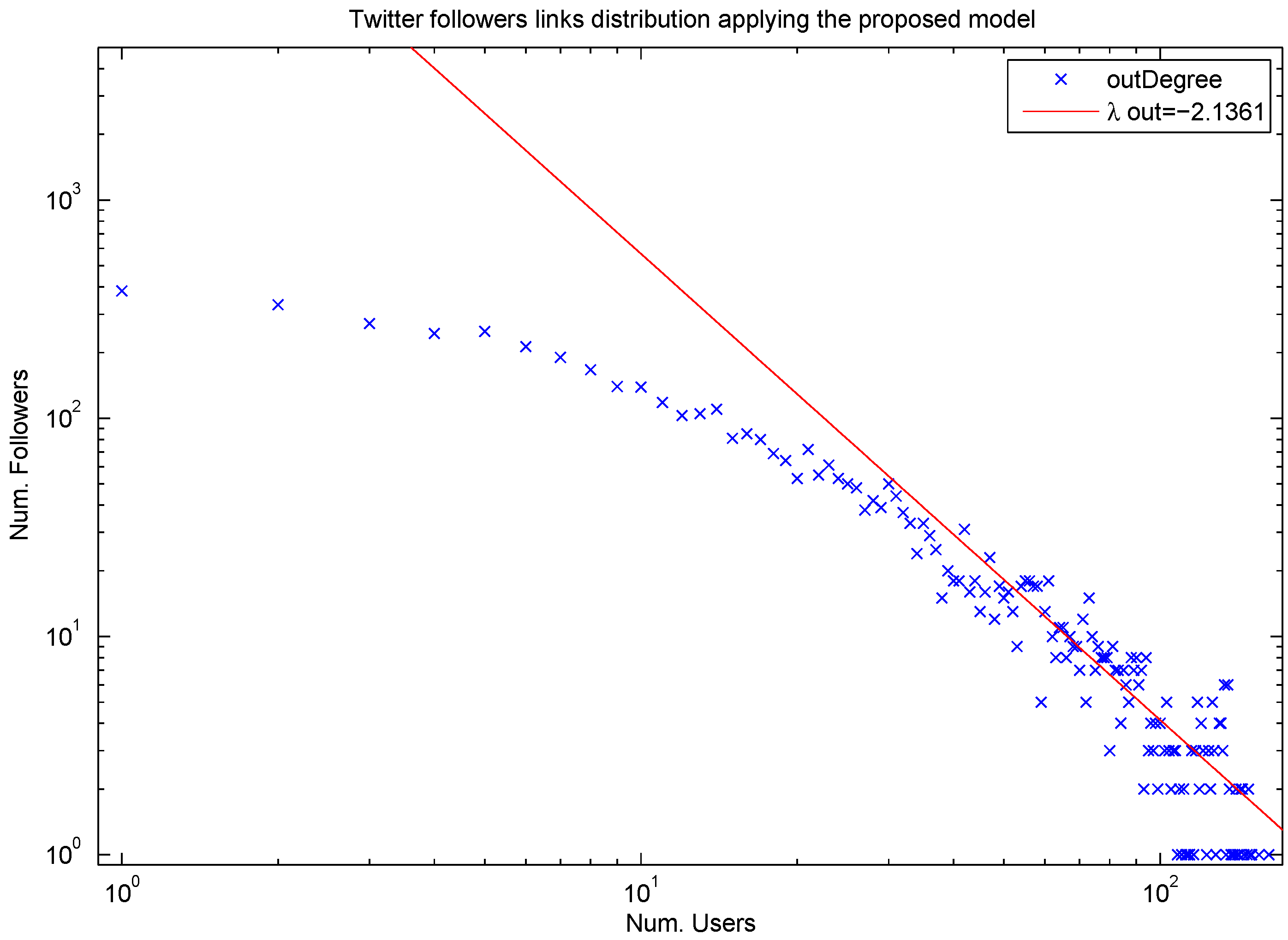
The proposed model was applied to generate a Twitter network of 5000 nodes considering the probability, p, of creating a new node attaching to a directed node equal to $0.016$. For these initial conditions, a total number of 98,324 links were created by the model. The degree distributions provided by the model are represented in Figure 8 and Figure 9. It is observed that the power law distribution follows the same trend as the ones obtained with real data in Section 3.2. It is shown that the model describes the “rich gets richer” philosophy, since new nodes are more likely to connect to high degree nodes than to low degree nodes. Therefore, it is concluded that our model is able to generate the power law behavior of the Twitter social network.

Figure 8. Outgoing degree distribution of Twitter’s network computed considering 5000 nodes with the proposed model.

Figure 8. Outgoing degree distribution of Twitter’s network computed considering 5000 nodes with the proposed model.

Figure 9. Incoming degree distribution of the Twitter network computed considering 5000 nodes with the proposed model.

Figure 9. Incoming degree distribution of the Twitter network computed considering 5000 nodes with the proposed model.

The clustering coefficient was also calculated. In Table 2, a comparison between the parameter values obtained with the real Twitter database and with the Twitter network generated by the proposed model for 5000 nodes is shown. It should be noticed that the value of the clustering coefficient is lower in the modeled Twitter, because the size of the generated network is smaller. Then, the following question arises about what is the minimum number of nodes required to properly generate a simulated Twitter network. This interesting aspect is out of the scope of this paper and could be the subject of future work.

Table 2. Comparison between the real Twitter network of $51,217,936$ users and the modeled network using 5000.

	${\lambda }_{\mathrm{IN}}$	${\lambda }_{\mathrm{OUT}}$	Clustering Coeff.
Real Twitter network	$-1.8778$	$-2.1715$	$0.096$$(9.6\%)$
Modeled Twitter network	$-1.8227$	$-2.1361$	$0.020$$(2\%)$

Table 2. Comparison between the real Twitter network of $51,217,936$ users and the modeled network using 5000.

	${\lambda }_{\mathrm{IN}}$	${\lambda }_{\mathrm{OUT}}$	Clustering Coeff.
Real Twitter network	$-1.8778$	$-2.1715$	$0.096$$(9.6\%)$
Modeled Twitter network	$-1.8227$	$-2.1361$	$0.020$$(2\%)$

As previously said, Twitter is one of the most popular social networks for spreading ideas. It has revolutionized the way millions of people consume news. Twitter is the world’s fourth-largest social network, so it is no surprise that Twitter malware attacks are on the rise. Therefore, this model can be applied to define an optimal defense strategy to fight against malware and spam spreading.

Twitter is also evolving into a major marketing tool in different areas of media and marketing. Therefore, it is important to find the best strategy for that purpose. With this model, it is possible to simulate a Twitter network and to analyze the way that messages are spread to find the best strategy to disseminate the required business information.

6. Conclusions

In this paper, we have studied the behavior of the Twitter social network. It was proven that Twitter can be considered as a scale-free network fulfilling the small world property. For that purpose, the degree distribution, the clustering coefficient and a conservative estimate of the average path length of the Twitter network have been computed using data as of September 2009 amounting to some 50 million users. Given this great number of users, a new heuristic method is introduced to estimate the average path length. This method consists of computing an upper bound dividing the network into two parts: the hub subnetwork (comprised of 1000 highly-connected nodes), and the rest. For any pair of nodes, a breadth-first algorithm searched then for a path via the hub subnetwork in three steps: from the initial node to a hub, from the hub subnetwork to the final node and within the hub subnetwork. The maximum path length in the hub subnetwork was found to be three. The numerical results confirm that Twitter, as other important real-world networks, is a scale-free, small world network with a high clustering coefficient. Such networks, not complying with the characteristic of geometrically-regular graphs, nor random graphs, are called complex networks.

A model has also been proposed considering developing networks with directed links based on the works of [10]. Our model is a generalization of the BA model to describe the behavior of social networks, which offers a more realistic point of view by considering also the creation of new links between old nodes. The proposed model has been applied to simulate the growth of Twitter. A Twitter network of 5000 nodes was generated creating 98,324 links. It was shown that the model describes the “rich gets richer” philosophy, and it was concluded that the model is able to generate the power law behavior of the Twitter social network; this modeled network can be used for different applications, for example marketing studies, malware and spam spreading, news dissemination, etc.

The clustering coefficient was also computed for this modeled network. The results obtained differ from the ones obtained with the real database, because the size of this network is smaller. A very interesting question arises, which is out of the scope of this paper, about what it is the minimum number of users necessary to describe the Twitter network. This fascinating aspect could be the subject of future work.