Detection of Causality between Process Variables Based on Industrial Alarm Data Using Transfer Entropy

Abstract

In modern industrial processes, it is easier and less expensive to configure alarms by software settings rather than by wiring, which causes the rapid growth of the number of alarms. Moreover, because there exist complex interactions, in particular the causal relationship among different parts in the process, a fault may propagate along propagation pathways once an abnormal situation occurs, which brings great difficulty to operators to identify its root cause immediately and to take proper actions correctly. Therefore, causality detection becomes a very important problem in the context of multivariate alarm analysis and design. Transfer entropy has become an effective and widely-used method to detect causality between different continuous process variables in both linear and nonlinear situations in recent years. However, such conventional methods to detect causality based on transfer entropy are computationally costly. Alternatively, using binary alarm series can be more computational-friendly and more direct because alarm data analysis is straightforward for alarm management in practice. The methodology and implementation issues are discussed in this paper. Illustrated by several case studies, including both numerical cases and simulated industrial cases, the proposed method is demonstrated to be suitable for industrial situations contaminated by noise.

1. Introduction

Alarms are indications of abnormal situations in process industries, including food, beverages, chemicals, pharmaceuticals, petroleum, ceramics, base metals, coal, plastics, rubber, textiles, tobacco, wood and wood products, paper and paper products, etc, where the primary production processes are either continuous or occur on a batch of materials that is indistinguishable [1]. In former times, due to the limitations of high cost and low quality of industrial monitoring systems, alarms have been configured via directly placing sensors to measure the physical quantity that needed to be monitored and transmitting the measurements to the control panel through cables. This caused the number of alarms at that time to remain at a low level. However, with the development of monitoring systems, modern plants in process industries have a multitude of sensors that are recorded and archived by process historians and monitored by distributed control systems (DCSs), supervisory control and data acquisition (SCADA) systems or other monitoring systems. Thus, most of the process variables can be configured to have at least one alarm and, in many cases, more than one. For example, for monitoring a pressure variable, four alarm tags can be configured, namely high-high, high, low and low-low. As a result, the number of alarm variables is often quite large, and hence, a large number of alarms are raised during an abnormal situation. Moreover, there often exist complex interactions between the corresponding process variables due to the process dynamics and the associated monitoring systems. Once an abnormal situation occurs at some place in the process, the fault may spread to many other places through interconnections between variables and process units. Such a situation often leads to alarm floods. In this case, it is difficult for operators to identify the type of fault or to find its root cause to mitigate the source of the abnormality. Without proper actions, such a situation may lead to serious and catastrophic events.

For example, in 1994, before an explosion accident happened in a fluid catalytic cracking unit of a refinery of British Texaco Company, there were 1775 out of 2040 alarm tags set to be “high priority” in DCS, and 275 alarms occurred in the last ten minutes, which caused operators not to take effective actions, leading to a major accident [2].

There are different ways to reduce the number of alarms, in particular nuisance alarms. For univariate methods, filtering, deadband, delay-timer and many other methods can be used [3].

On the other hand, for bivariate or multivariate situations, Folmer et al. [4] summarized several approaches. Among these approaches, it is an essential method to identify the propagation paths between variables and, thus, to localize the root cause of the abnormal situation. Yang et al. used signed directed graphs to identify the process topology and connectivity that help in fault diagnosis and process hazard assessment [5,6]. Noda et al. [7] and Yang et al. [8] used event correlation analysis to design a policy to reduce alarms. Using causality information between alarm variables is another approach in this area. Thereby, the propagation path of the fault can be found, and this will help operators identify the root cause [9]. This enables operators to take preventative actions immediately. Thus, the detection of causality between variables becomes important and has received a lot of attention.

The first experimental example of causality detection by analyzing consecutive time series was demonstrated by Granger [10]. He formalized the causality identification idea in linear regression models by the following thought: we consider that there exists causality from random variable I to J if the variance of the autoregressive prediction error of J can be reduced by additionally considering the historical data of I.

After that, some more advanced techniques for causality identification have been proposed by different researchers, such as extended Granger causality [11], nearest neighbor methods [12] and transfer entropy (TE) [13].

Among these methods, TE, which was proposed by Schreiber in 2000, has been considered a useful way to describe causality between variables. The major advantage of TE is that it can be used in both linear and nonlinear situations. What is more, TE is equivalent to Granger causality in the presence of Gaussian noise [14], which indicates that TE is also consistent with the concept of causality in the predictive Granger sense. Since its introduction, TE has been successfully applied to industrial data to identify causal relationships between process variables [15]. With the further development of TE, there have been many extensions for causality identification. For example, Duan et al. extended the traditional concept of TE and made it more applicable, especially for multivariate cases [16,17]. Yang et al. [18] and Duan et al. [19] also summarized these methods for capturing causality in industrial processes.

However, TE has primarily been used for continuous time series, which can describe the whole characteristic of the process, but is computationally quite burdensome. In the context of alarm management, causality under abnormal situations is usually of more concern rather than the exact dynamic relationships under all situations. Therefore, it is unnecessary to take all cases (all situations and process data) into account, and we would rather just focus on processing data in abnormal situations (typically processing alarm data). In addition, because some alarm variables themselves are not generated by continuous variables, such as switch variables (e.g., ON/OFF for a pump) and state variables, a discrete version of TE is needed. Considering the computational cost and the above issues, it is reasonable to detect causality between variables using alarm data directly.

Although there are already some discrete extensions of TE (for example, Staniek et al. proposed symbolic transfer entropy to reduce the computational burden to estimate TE [20]), our purpose is not the same. The main reason for emphasizing the discrete version of TE is that alarm data are binary by nature. For analogue alarms, the corresponding process values are compared to the thresholds for discretization. Thus, it is natural to use such binary alarm data for causality detection.

The main contribution of this paper is a new application of TE to identify causality between variables by using binary alarm data in general multivariate systems. The proposed method and the above-mentioned methods are compared in both variable type and their main characteristic, as shown in Table 1. It can be seen that the types of methods used for the discrete situation are far fewer than methods for the continuous situation, especially using such binary alarm data, which makes the method easy to use.

The rest of this paper is organized as follows. In Section 2, the basic definition of transfer entropy is revisited, and related concepts are also introduced. The TE method based on binary alarm data is proposed in Section 3. Several simulated case studies are given in Section 4 to show the effectiveness of the proposed method for detecting the causality between variables, followed by concluding remarks in Section 5.

Table 1. The comparison of the mentioned methods and the proposed method. TE, transfer entropy.

Method	Authors	Variable Type	Main Characteristic
signed directed graph	Yang, Shah and Xiao [5,6]	continuous	qualitative model to detect the cause and effect relationship
event correlation analysis	Noda, Higuchi, Takai and Nishitani [7]	continuous	a data mining method to detect statistical similarities
Granger causality	Granger [10]	continuous	based on AR models
extended Granger causality	Ancona, Marinazzo and Stramaglia [11]	continuous	nonlinear extension of Granger causality
nearest neighbor methods	Bauer, Cox, Caveness, Downs and Thornhill [12]	discrete	data-driven and operating on the process measurements stored in a data historian
transfer entropy	Schreiber [13]	continuous	based on information theory
direct transfer entropy	Duan, Yang, Chen and Shah [16]	continuous	extension of TE to detect direct relationship
transfer zero-entropy	Duan, Yang, Shah and Chen [17]	continuous	avoid estimating high dimensional pdfs using 0-entropy
symbolic transfer entropy	Staniek, Lehnertz [20]	discrete	avoid estimating high dimensional pdfs using a technique of symbolization
this paper		discrete	use natural binary alarm data for causality detection

Table 1. The comparison of the mentioned methods and the proposed method. TE, transfer entropy.

Method	Authors	Variable Type	Main Characteristic
signed directed graph	Yang, Shah and Xiao [5,6]	continuous	qualitative model to detect the cause and effect relationship
event correlation analysis	Noda, Higuchi, Takai and Nishitani [7]	continuous	a data mining method to detect statistical similarities
Granger causality	Granger [10]	continuous	based on AR models
extended Granger causality	Ancona, Marinazzo and Stramaglia [11]	continuous	nonlinear extension of Granger causality
nearest neighbor methods	Bauer, Cox, Caveness, Downs and Thornhill [12]	discrete	data-driven and operating on the process measurements stored in a data historian
transfer entropy	Schreiber [13]	continuous	based on information theory
direct transfer entropy	Duan, Yang, Chen and Shah [16]	continuous	extension of TE to detect direct relationship
transfer zero-entropy	Duan, Yang, Shah and Chen [17]	continuous	avoid estimating high dimensional pdfs using 0-entropy
symbolic transfer entropy	Staniek, Lehnertz [20]	discrete	avoid estimating high dimensional pdfs using a technique of symbolization
this paper		discrete	use natural binary alarm data for causality detection

2. Concept of Transfer Entropy

In this section, the basic definition of TE is described. In addition, estimation methods and some related concepts are also presented.

2.1. Basic Definition

Given two continuous random variables I and J, let them be sampled at time instant t and denoted by $i_t\in [i_{\mathtt{min}},i_{\mathtt{max}}]$ and $j_t\in [j_{\mathtt{min}},j_{\mathtt{max}}]$ with $t=1,2,\cdots ,N$, where N is the number of time bins.

Let $i_{t+h}$ denote the value of I at time instant $t+h$, which means h steps in the future from t, and h is called the prediction horizon. Let ${\mathbf{i}}_t^{\left(k\right)}=[i_t,i_{t-\tau },\cdots ,i_{t-(k-1)\tau }]$ denote the embedded vectors with elements being the past values of I; ${\mathbf{j}}_t^{\left(l\right)}=[j_t,j_{t-\tau },\cdots ,j_{t-(l-1)\tau }]$ the embedded vectors with elements being the past values of J (thus, k is the embedding dimension of I, and l is the embedding dimension of J); τ is the time interval, which can allow us to sample the embedded vector; $f(i_{t+h},{\mathbf{i}}_t^{\left(k\right)},{\mathbf{j}}_t^{\left(l\right)})$ the joint probability density function (pdf) of $i_{t+h}$, ${\mathbf{i}}_t^{\left(k\right)}$ and ${\mathbf{j}}_t^{\left(l\right)}$; $f\left(i_{t+h}\right|{\mathbf{i}}_t^{\left(k\right)},{\mathbf{j}}_t^{\left(l\right)})$ the conditional pdf of $i_{t+h}$ given ${\mathbf{i}}_t^{\left(k\right)}$ and ${\mathbf{j}}_t^{\left(l\right)}$; and $f\left(i_{t+h}\right|{\mathbf{i}}_t^{\left(k\right)})$ the conditional pdf of $i_{t+h}$ given ${\mathbf{i}}_t^{\left(k\right)}$ only. The differential TE (TE${}_{\mathtt{diff}}$) from J to I, for continuous random variables, is estimated as follows:

$$\begin{array}{c}\hfill T{E}_{J\to I}=\int f(i_{t+h},{\mathbf{i}}_t^{\left(k\right)},{\mathbf{j}}_t^{\left(l\right)})log\frac{f\left(i_{t+h}\right|{\mathbf{i}}_t^{\left(k\right)},{\mathbf{j}}_t^{\left(l\right)})}{f\left(i_{t+h}\right|{\mathbf{i}}_t^{\left(k\right)})}d\mathbf{w},\end{array}$$

(1)

where $\mathbf{w}$ denotes the random vector $[i_{t+h},{\mathbf{i}}_t^{\left(k\right)},{\mathbf{j}}_t^{\left(l\right)}]$. If we assume that the elements of $\mathbf{w}$ are $w_1,w_2,\cdots ,w_s$, then $\int (•)d\mathbf{w}$ denotes ${\int }_{-\infty }^{\infty }\cdots {\int }_{-\infty }^{\infty }(•)d{w}_1\cdots d{w}_s$. Here, the numerator of the logarithm expression, which is the conditional pdf of $i_{t+h}$ given ${\mathbf{i}}_t^{\left(k\right)}$ and ${\mathbf{j}}_t^{\left(l\right)}$, represents the prediction result of the value of I when the historical data of both I and J are known; the denominator of the logarithm expression, which is the conditional pdf of $i_{t+h}$ given ${\mathbf{i}}_t^{\left(k\right)}$, represents the prediction result of the value of I, when only the historical data of I itself is known. Thus, the idea of TE is that if there exists causality from J to I, it will be helpful to predict the value of I using the historical data of J; then, the value of the numerator should be greater than the value of the denominator, and the value of the whole estimation equation should be greater than zero; if there does not exist causality from J to I, the value of the whole equation should be close to zero. From another point of view, the estimated result of TE can be considered as the information for the future observation of I obtained by discarding the information about the future of I obtained from the past values of I alone from the simultaneous observations of both the past values of I and J.

However, as TE${}_{\mathtt{diff}}$ is defined for continuous random variables and, yet in real industrial cases, sampled time series data are always used to describe continuous random variables, the formula of a discrete version of TE for quantized sample data, i.e., TE${}_{\mathtt{disc}}$, needs to be used.

2.2. Discrete Version of TE

For continuous random variables I and J, let $\tilde{I}$ and $\tilde{J}$ denote the quantized I and J, respectively. Assume that the ranges of I and J, which are denoted as $[i_{\mathtt{min}},i_{\mathtt{max}}]$ and $[j_{\mathtt{min}},j_{\mathtt{max}}]$, are divided into $n_i$ and $n_j$ non-overlapping bins, respectively, and let ${\Delta }_i$ and ${\Delta }_j$ denote the corresponding quantization bin sizes of I and J, respectively. If a uniform quantization is used, we can have:

$$\begin{array}{c}\hfill {\Delta }_i=\frac{i_{\mathtt{max}}-i_{\mathtt{min}}}{n_i-1},\end{array}$$

(2)

for I as an example. Here, the quantization bin size is related to the range of the variable and the number of quantization bins. When the range of the variable is given, if we want to obtain a smaller quantization bin size, the number of quantization bins has to be larger. Then, the TE${}_{\mathtt{diff}}$ from J to I can be approximated by the TE${}_{\mathtt{disc}}$ from $\tilde{J}$ to $\tilde{I}$, that is:

$$\begin{array}{c}\hfill T{E}_{\tilde{J}\to \tilde{I}}=\sum p({\tilde{i}}_{t+h},{\tilde{\mathbf{i}}}_t^{\left(k\right)},{\tilde{\mathbf{j}}}_t^{\left(l\right)})log\frac{p\left({\tilde{i}}_{t+h}\right|{\tilde{\mathbf{i}}}_t^{\left(k\right)},{\mathbf{j}}_t^{\left(l\right)})}{p\left({\tilde{i}}_{t+h}\right|{\tilde{\mathbf{i}}}_t^{\left(k\right)})},\end{array}$$

(3)

where the meanings of the symbols in this equation is similar to those in Equation (1).

With some mathematical derivations similar to those in [16], the TE${}_{\mathtt{diff}}$ from J to I is almost the same as the TE${}_{\mathtt{disc}}$ from $\tilde{J}$ to $\tilde{I}$ as the quantization bin sizes of I and J tend to zero, which means that the TE${}_{\mathtt{disc}}$ is an estimator of the TE${}_{\mathtt{diff}}$.

For choosing the quantization bin size, there is a tradeoff between the quantization accuracy and computational burden in the traditional methods. That is, the smaller the bin size chosen, the more accurate is the quantization and the closer TE${}_{\mathtt{disc}}$ is to TE${}_{\mathtt{diff}}$; yet, on the other hand, the computational burden, especially the summation and the probability estimation parts, will increase significantly with the smaller bin size, which means larger quantization bin numbers.

In this paper, a binary alarm series is suggested to use to estimate the TE${}_{\mathtt{disc}}$, which means the bin numbers of I and J are chosen as $n_i=n_j=2$, and thus, bin sizes ${\Delta }_i$ and ${\Delta }_j$ are equal to the full ranges of I and J, respectively. In other words,

$$\begin{array}{c}\hfill \left\{\begin{array}{c}{\Delta }_i=i_{\mathtt{max}}-i_{\mathtt{min}}\hfill \\ {\Delta }_j=j_{\mathtt{max}}-j_{\mathtt{min}}\hfill \end{array}\right..\end{array}$$

(4)

In addition, when continuous data are normalized to 0–1 series, this can be seen as the type of alarm series. The main advantage of choosing the quantization bin sizes in this way is that it can significantly reduce the computational burden, because in this way, one can avoid the estimation of a high dimensional pdf.

Overall, binary alarm series are suggested for the following reasons: The first reason is obviously the computational burden. In [16], the TE${}_{\mathtt{diff}}$ is directly used to estimate TE in order to avoid the round-off error. Mathematical techniques are used to estimate the TE${}_{\mathtt{diff}}$, which express the conditional pdfs by joint pdfs and, thus, can be obtained by the kernel estimation method. For q-dimensional multivariate data, the Fukunaga method [21] is used to estimate the joint pdf. As can be seen, the computational burden is relatively high just because of the kernel estimation of the joint pdfs. If the binary alarm series are used, the computational burden will be decreased significantly to an acceptable level.

The second reason is that the causality under abnormal situations is often of more concern rather than the exact dynamic relationships under normal situations in the context of alarm management. Usually, the information under abnormal situations is still contained in the binary alarm data, although most information is lost. Thus, taking all of the situations or all of the process data into account is unnecessary, and the processing of data in abnormal situations (typically only processing alarm data) is our focus.

The last reason is that in industrial processes, not all alarms are generated by quantizing continuous series. For example, switch variables (e.g., ON/OFF) and state indicators often describe the manual operations or the sudden changes in some units; they generate digital alarms. Thus, a discrete version of TE can be applied.

Considering the above issues, the causality between variables can be detected using alarm data directly.

2.3. Required Assumptions

Since the concept of TE is still employed, the assumptions required here are exactly the same as those for continuous TE. Two assumptions are required: there should be sufficient relevant data points to estimate the probability density function of data; the time series used should be stationary in a wide sense, which requires that all of the dynamical properties of the process cannot change during the whole sampled data period [22,23].

The first assumption is rather easy to satisfy, while the second one should be tested before estimating TE. However, in most cases, the process cannot be directly accessible, and the only information that can be obtained is from the sampled data. Thus, in order to test the stationarity, the simplest and most widely-used way is to measure whether the mean, the variance and the auto-correlation of the time series are time-independent.

3. Transfer Entropy Based on Alarm Data

In this section, a method is proposed to estimate the TE based on alarm data. The brief procedure is shown in Table 2.

Table 2. The procedure to detect causality between industrial alarm series based on TE.

1	Obtain the original data;
2	Preprocess data and obtain series I, J;
3	Estimate the TE${}_{JI}$ = TE$(I,J,k,l)$;
4	for t = 1:reptime{
5	$J^{\prime }$ = surrogate(J);
6	Estimate the TE${}_t$ = TE$(I,J^{\prime },k,l)$;
7	}
8	$threshold$ = $P_{95}$($F_n$(TE${}_t$));
9	Compare TE${}_{JI}$ with $threshold$

Table 2. The procedure to detect causality between industrial alarm series based on TE.

1	Obtain the original data;
2	Preprocess data and obtain series I, J;
3	Estimate the TE${}_{JI}$ = TE$(I,J,k,l)$;
4	for t = 1:reptime{
5	$J^{\prime }$ = surrogate(J);
6	Estimate the TE${}_t$ = TE$(I,J^{\prime },k,l)$;
7	}
8	$threshold$ = $P_{95}$($F_n$(TE${}_t$));
9	Compare TE${}_{JI}$ with $threshold$

3.1. Alarm Series and Data Collection

(1) Format of the alarm series: As mentioned above, up to now, continuous process data have been used in most studies to detect causality between variables using TE. However, in this paper, alarm series or event series are used. Actually, the so-called alarm series used here is a generalized concept, which may include not only the common alarm series, but also other types of binary series. In such binary series, there are two possible values at each sampling instant, i.e., zero and one. There are two ways to present alarms [24]. The first way is just setting the start time of alarms “1”, and the other way is setting all of the time instants with alarms “1”. As there are numerous false and missed alarms in a real situation, it is inaccurate to just use the start time. Moreover, when there are many variables with alarms, it is difficult to say which alarm tags are related. However, the second way converts the alarm sequences into binary sequences with “0’s” and “1’s” representing normal and abnormal situations, respectively. Such a method is suitable for the pdf estimation. Therefore, in this report, zero represents no alarm, and one represents an alarm. Note that the binary series or the alarm series here just simply shows whether there is an alarm or not, as generated by the DCS system according to some configuration, while it does not show whether there is a fault or an abnormal situation. A false alarm or a false positive is one where there is an alarm, but there is no fault, while a missed alarm or a false negative is one where there is a fault, but an alarm is not raised. The difference can be caused by many reasons, such as noise.

(2) Comparison of the alarm series in different areas: Although continuous process data are used in most of the literature, binary series are also used in different areas. For example, in neuroscience, Ito et al. used a binary electrical signal series to detect causality [25].

Although these binary series used in different areas are all composed of 0–1 digits, there are different characteristics of them.

Firstly, because electrical signals in neuroscience are usually used to transmit the instructions from one nerve cell to another with stimulations, they only exist in a very short time period like spikes. Thus, the series of electrical binary signals are often very sparse, and people put more emphasis on the start time of signals; while alarms in industrial processes usually mean the change from the normal state to an abnormal state of the process; so, they often last for a period of time, and once an abnormal situation occurs, the alarms will probably be intensive.

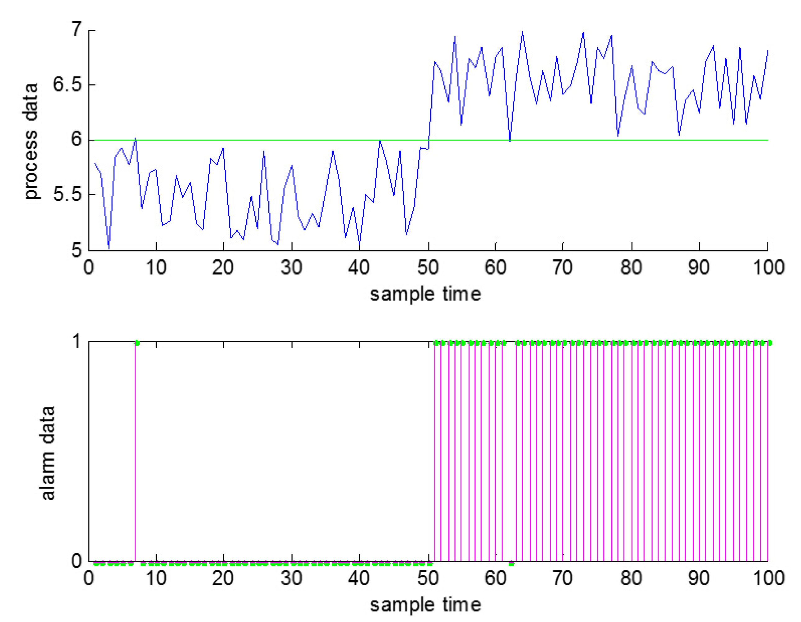
On the other hand, electrical signals in neuroscience are usually clean, because they just transmit the instructions between neurons; while there are often some false alarms and missed alarms in industrial processes when using the thresholds to generate the alarms due to the existence of noise [26], just as shown in Figure 1. As a result, false alarms and missed alarms will bring some wrong information into the alarm data, which in other words will reduce the amount of information that can be obtained from the data.

Figure 1. False alarms and missed alarms generated by noise (a false alarm at $t=7$, a missed alarm at $t=62$).

Figure 1. False alarms and missed alarms generated by noise (a false alarm at $t=7$, a missed alarm at $t=62$).

Since we cannot change the thresholds or use deadband or delay timers to change the alarm series here, like the methods in process data, some other methods of data preprocessing are needed before using industrial data for analysis in order to reduce the rates of false alarms and missed alarms.

(3) Collection of the alarm data: The alarm data can be obtained in different ways according to the different kinds of cases. For stochastically-simulated cases, we can either generate the continuous process data first and then convert them into binary alarm data with appropriate thresholds or generate discrete binary series directly by software configuration. Under this situation, abnormal states can be set freely as one wishes. For real industrial processes, discrete binary series can be obtained directly using DCS. In this way, alarms are usually listed in the logs in some specific format, which may include some key information of the alarms, such as the start time of the alarm, the name of the variable, the type of the alarm and so on. Thus, log files need to be converted to binary series before using them. Even more, there may be more complex circumstances in real industrial processes, including noise and other disturbances. However, this type of binary series can reflect more information in real industrial processes than in stochastic examples. Thus, the proposed method should be tested with both simulated cases and real industrial cases to testify its effectiveness.

3.2. Data Preprocessing

As mentioned above, because of the high rates of false alarms and missed alarms caused by noise and other disturbances, data preprocessing is essential before the estimation of TE.

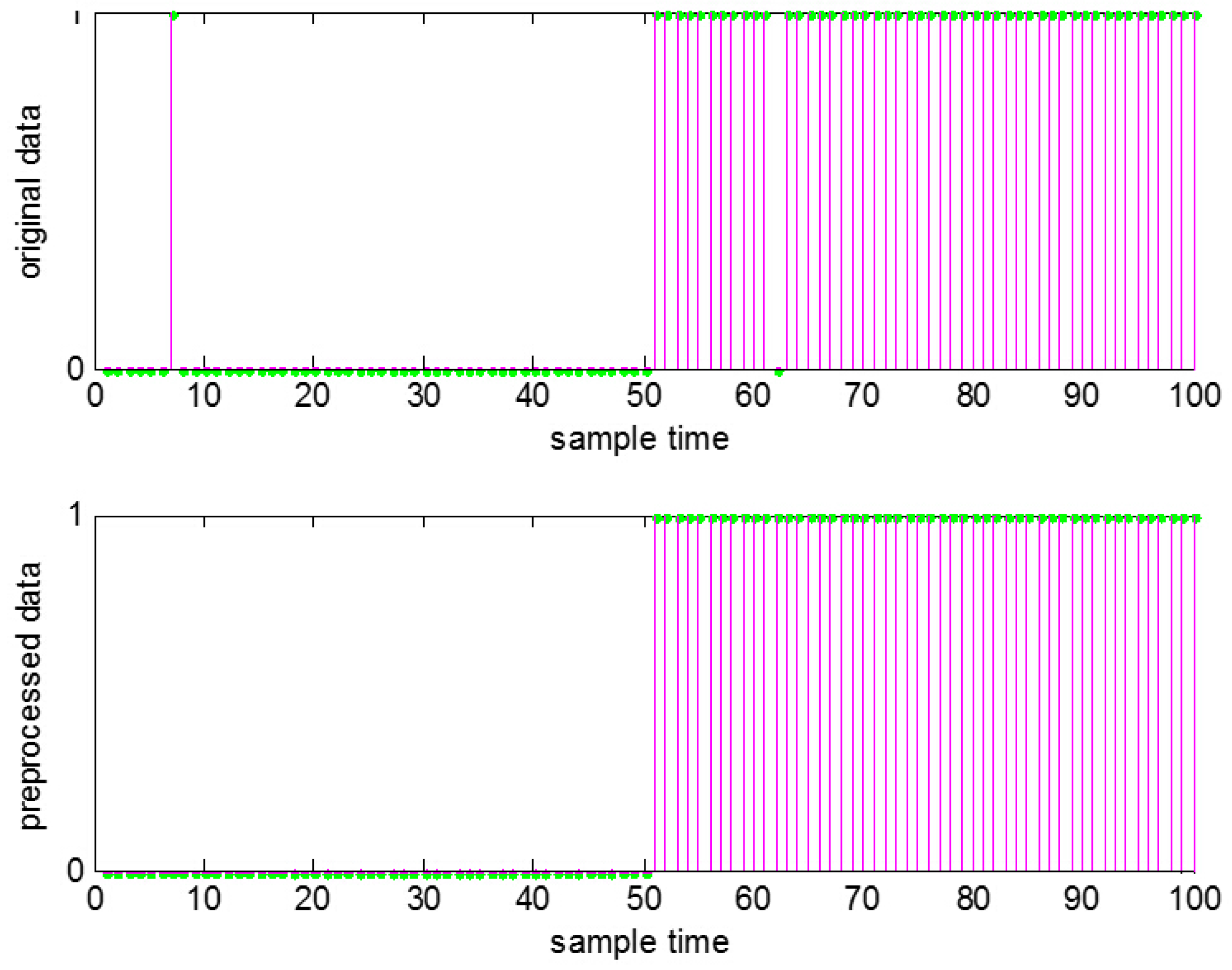
Filtering is a widely-used and effective way to reduce noise, among which the moving average method is the most simple and common one. Thus, the moving average method is chosen here. With such data preprocessing, usually the number of false and missed alarms can be observably reduced, and thus, the information obtained from the binary alarm series can be improved. The result for Figure 1 after the data preprocessing is shown in Figure 2.

Figure 2. Data preprocessing to remove false and missed alarms.

Figure 2. Data preprocessing to remove false and missed alarms.

Some discussions for data processing are given below:

(1)

Interpretation of the preprocessing: The starting point to use the moving average method is quite natural. Generally speaking, the state of a real industrial process will last for quite a long time, no matter if in the normal state or the abnormal state. For that reason, those single alarms with no other alarms before or after them over a long period of time are more likely to be considered as false alarms caused by noise, which is different from those similar single signals or “spikes” in neuroscience, while alarmless time bins surrounded by alarms are more likely to be considered as missed alarms. Furthermore, these false alarms or missed alarms can be seen as originating from high-frequency variables, and with the moving average method, they can be reduced significantly.

(2)

Determination of the parameters: The window width u should be determined in the algorithm. However, u is influenced by several factors. The first one is the property of the industrial process itself, which means the structure and the operation mode of the process, such as whether it is a fast process or a slow process. If it is a slow process, which means the measured value changes slowly, both the normal state and the abnormal state will last for a longer time, and the influence of the noise is smaller, so u can be set to a larger value to improve the accuracy. If it is a fast process, u should be set small. The second factor is the sampling interval. If the interval is large, u should be set small in order not to lose more information of the process, otherwise u can be set large. Furthermore, the total length of the time series should be considered, and the ISA (The International Society of Automation) 18.2 standard [27], in which the limit of an alarm flood is 10 alarms per 10 min, should be met. Thus, the determination of u is quite complex.

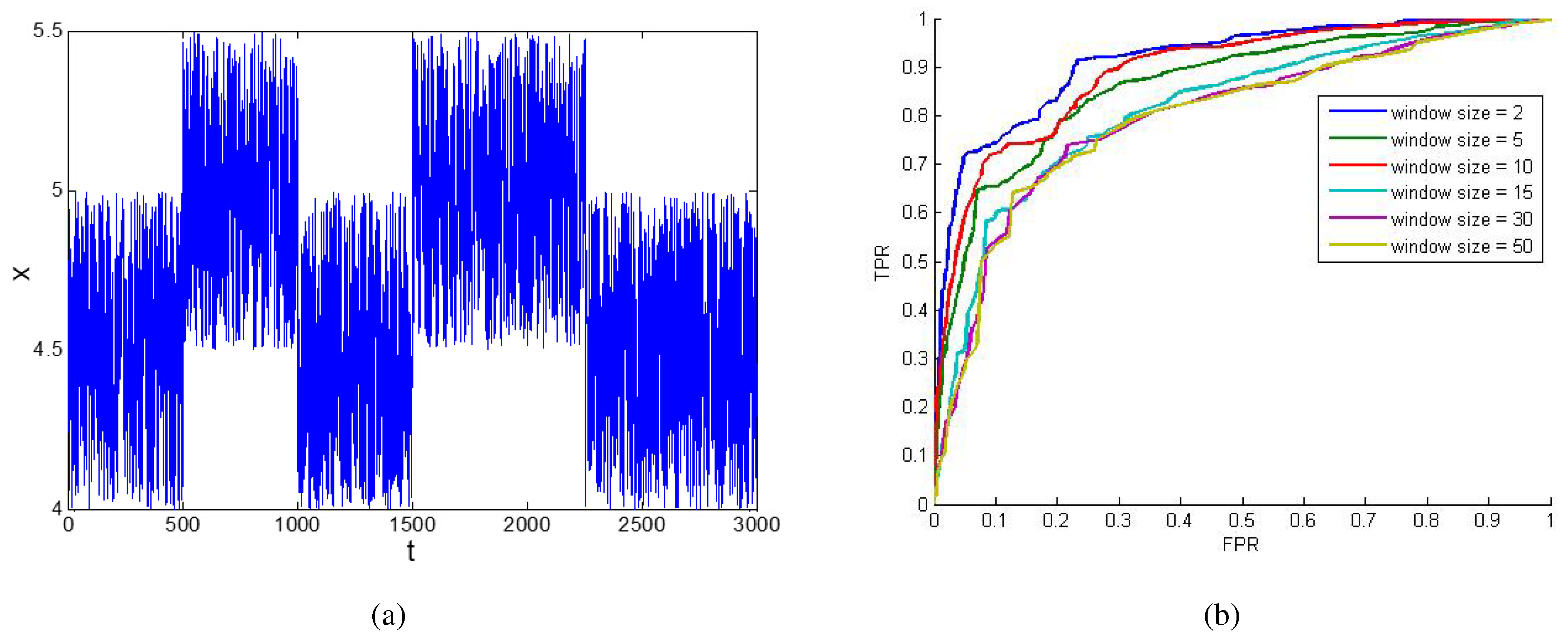
Here, an experiment is made to show the impact of u when using the moving average method. In Figure 3a, x is a continuous random variable, and there are two abnormal situations during the whole time period. When it is converted into binary series using different thresholds, the false positive rate (FPR) and the true positive rate (TPR) in the result will be different. Thus, a receiver operating characteristic (ROC) curve with FPR as the X axis and TPR as the Y axis can be drawn. Such a binary series is just the original data we need. Then, the moving average method can be used to preprocess the original data. When different u values are chosen, different results and, thus, different ROC curves can be obtained, as shown in Figure 3b. It can be seen that the curves with small u are closer to the upper-left corner, which means the effect of the filtering is better. The area under the curve (AUC) criterion for $u=[2,5,10,15,30,50]$ in Figure 3b is [0.9133, 0.8633, 0.8912, 0.8148, 0.7984, 0.7955], respectively. Thus a u smaller than 10 might be a better choice.

Figure 3. The impact of u of the moving average filters. (a) A random time series x; (b) the ROC curve of x by using moving average filters with different u.

Figure 3. The impact of u of the moving average filters. (a) A random time series x; (b) the ROC curve of x by using moving average filters with different u.

There is one point worth noting: in order to meet the stationarity assumption, the series are in steady states, rather than in transitional states, which means that the transitional period from the normal state to abnormal state or in the opposite direction should be chosen.

3.3. Estimation of TE

After finishing the data preprocessing, the validated data are obtained. Then, the TE can be estimated, and the causality between variables can be detected using these preprocessed binary series. Here, the preprocessed series of variables I and J is taken as an example.

(1) Estimation of first-order TE: For each pair of variables I and J, to estimate TE from J to I, there are two main steps. The first step is to estimate the pdfs in Equation (3). The second step is to compute the TE with the pdfs estimated by using Equation (3).

It is easy to see that the first step is more important and more computationally expensive. For this reason, binary series are used instead of continuous process data to reduce the computational cost. As the traditional pdf can be expressed with joint pdfs, only the joint pdf needs to be estimated here. As binary series are used, the number of possible values of $p({\tilde{i}}_{t+h},{\tilde{\mathbf{i}}}_t^{\left(k\right)},{\tilde{\mathbf{j}}}_t^{\left(l\right)})$ is reduced from a huge amount to merely $2^{l+k+1}$ possible patterns. For first-order TE, i.e., $k=l=1$, there are only $2^3=8$ possible patterns. Thus, it is unnecessary to use a kernel estimation method or other complex mathematical methods to estimate the high dimensional joint pdfs in the equation. Instead, the numbers of each possible patterns of the joint pdf need to be counted.

In order to estimate the TE between two variables, the most computationally-costly part is to estimate the joint pdf, which is our first step.

Assume that the number of time bins is N; then, the computational cost to estimate the joint pdf can be seen as growing linearly in N. Even more, the computational cost of this part is almost the majority of all of the cost to estimate TE. Thus, the total computational cost to estimate TE for each pair of variables grows linearly in N, i.e., $O\left(N\right)$.

(2) Higher-order TE estimation: For higher orders of TE estimation, the method is a generalization of the first-order method.

The complexity of higher-order TE is also very similar. Except for the number of time bins, the total order r($=l+k+1$) is also an important factor to affect the computational cost. As there are $r=l+k+1$ series to be considered and $2^r$ possible patterns in total, r bits need to be examined, which will make a linear complexity in $Nr$. After all frequencies of every possible pattern and the corresponding joint pdfs are obtained, they will be summed up, leading to a complexity of $2^r$. Thus, the total computational cost of the higher-order TE estimation for each pair of variables is $O(Nr+2^r)$.

(3) Determination of the parameters of TE: When TE is estimated to detect causality between variables, there are four parameters to be determined, namely h, τ, k, l, as shown in Section 2. As for h and τ, $h=\tau \le 4$ if the process dynamics are unknown is recommended in [15]. However, in fact, correlation properties can be used to estimate τ [28]. Anyway, in this manuscript, small h and τ are still used, as the cases used here are all of a small time delay. Thus, the rest of the work is just to determine the embedding dimensions k and l.

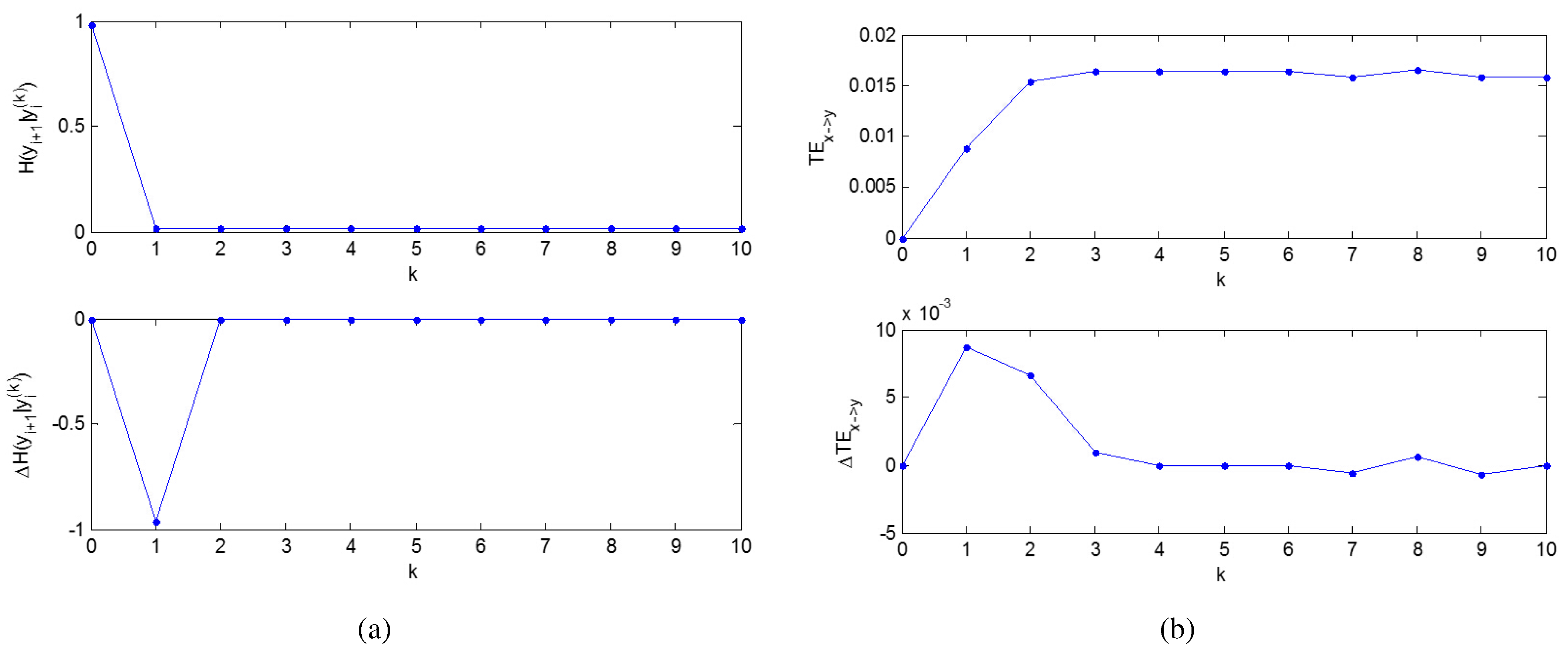
First, the embedding dimension k, which corresponds to the window size of the historical data of I itself used to predict the future I, should be determined. Here, the conditional Shannon entropy is used, i.e.,

$$\begin{array}{c}\hfill H\left({\tilde{i}}_{t+h}\right|{\tilde{\mathbf{i}}}_t^{\left(k\right)})=-\sum p({\tilde{i}}_{t+h},{\tilde{\mathbf{i}}}_t^{\left(k\right)})logp\left({\tilde{i}}_{t+h}\right|{\tilde{\mathbf{i}}}_t^{\left(k\right)}),\end{array}$$

(5)

which quantifies the amount of information obtained from historical data of I itself to predict future I with the current embedding dimension. Here, $p({\tilde{i}}_{t+h},{\tilde{\mathbf{i}}}_t^{\left(k\right)})$ denotes the joint probability mass function (pmf) of ${\tilde{i}}_{t+h}$ and ${\tilde{\mathbf{i}}}_t^{\left(k\right)}$; $p\left({\tilde{i}}_{t+h}\right|{\tilde{\mathbf{i}}}_t^{\left(k\right)})$ denotes the conditional pmf of ${\tilde{i}}_{t+h}$ given ${\tilde{\mathbf{i}}}_t^{\left(k\right)}$. Thus, the change rate of $H\left({\tilde{i}}_{t+h}\right|{\tilde{\mathbf{i}}}_t^{\left(k\right)})$ shows how much more information can be obtained at the price of the increase of the embedding dimension, which will increase the computational cost. Because the least computational cost possible is what is wanted to be used here, it is a good strategy for the determination of k, which can be determined as the minimum non-negative integer above which the change rate of $H\left({\tilde{i}}_{t+h}\right|{\tilde{\mathbf{i}}}_t^{\left(k\right)})$ decreases significantly.

Then, the embedding dimension l, which shows the window size of the historical data of J used to predict the future I, can be determined as the minimum positive integer above which the change rate of the TE from J to I decreases significantly.

3.4. Estimation of the Significance Level

The idea of TE is to detect whether the historical data of J are helpful to predict the value of I. If it is helpful, we can say that there exists causality from J to I, and thus, the TE result estimated by Equation (3) should be larger than zero; otherwise, the result should be zero. However, in real industrial processes, generally speaking, the estimated result of TE will not be exactly zero, because of the impact of noise or other disturbance, even if data preprocessing has already been made and such an impact has been reduced. For this reason, a threshold is needed to identify when the conclusion can be drawn that there is causality from J to I or, in other words, the significance level needs to be confirmed. In order to obtain such a threshold, Kantz and Schreiber suggested using a Monte Carlo method with surrogate data [29]. Monte Carlo methods solve the problem by generating appropriate random data with some desired property. The problem can then be considered as accepting or rejecting a null hypothesis. The null hypothesis here is that there exists no causality from J to I, implying that the TE is statistically indistinguishable from zero. On the contrary, if a large value for the TE result is estimated, the null hypothesis should be rejected.

When this method is used, the number of alarms in the time series for the variable J is kept while the sequence and occurrence times of these alarms are changed randomly, which generates a surrogate series $J^{\prime }$. Then, TE is estimated using I and $J^{\prime }$ with the procedure described in Section 3.2 andSection 3.3. Since the locations of alarms in $J^{\prime }$ are randomly generated, a possibly existing causality between series is removed, and the distribution of the estimated values of TE based on the surrogates can be used to estimate the significance threshold. In the experiment, we generate nsuch surrogate alarm series and obtain a series of TE values $T{E}_1,T{E}_2,\cdots ,T{E}_n$.

As the data obtained may not follow a normal distribution, it is recommended to take the 95% quantile of the empirical distribution of the series of TE values as the significance threshold.

$$\begin{array}{c}\hfill S_{JI}=P_{95}\left(F_n(T{E}_1,T{E}_2,\cdots ,T{E}_n)\right),\end{array}$$

(6)

where $P_{95}$ means the 95% quantile and $F_n\left(x\right)$ is the empirical distribution of the obtained TE values from the experiment.

When the estimated TE value exceeds this threshold, there exists significant causality from J to I.

However, the method used here may sometimes bring some new problems, especially when there are series of correlated events. In such circumstances, the shuffling procedure would destroy the relationships. Thus, it could be better to shuffle the events block-wise instead of individually.

4. Case Studies

In this section, two stochastic examples and one simulated industrial case are studied to show the effectiveness of the proposed method. In the stochastic examples, the causality between variables is expressed by simple mathematical equations. In the simulated industrial case, a benchmark simulation platform, the Tennessee-Eastman Process (TEP), is used.

4.1. Stochastic Processes

Example 1. The first case is described by the following equations:

$$\begin{array}{c}\hfill \left\{\begin{array}{c}{Y}_{k+1}=0.8X_k+0.2Y_k+v_{1k},\hfill \\ Z_{k+1}=0.6Y_k+v_{2k},\hfill \end{array}\right.\end{array}$$

(7)

where X, Y and Z are three continuous random variables, $v_{1k},v_{2k}\sim N(0,0.1^2)$, $X_k\sim N(0,1^2)$ in the normal situation and, then, a constant value of four added to X in the time intervals [501, 1000] and [1501, 2250] to realize abnormality; and then, Y and Z can be calculated according to Equation (7).

We convert these variables into binary alarm series with upper limits of normal states as thresholds, which are 2, 3, 2 for X, Y and Z, respectively, as shown in Figure 4.

It is known from Equation (7) that there exists direct causality from X to Y and Y to Z and indirect causality from X to Z. Yet, there is no causality from Y to X, Z to Y or Z to X.

To estimate the TE between x, y and z, the four parameters in Equation (3) need to be determined beforehand. Here, the TE from x to y is taken as an example. As mentioned above, $h=\tau =1$ is taken first. Then, $H\left(y_{t+1}\right|{\mathbf{y}}_t^{\left(k\right)})$ and its change rate with $k=0,1,\cdots ,10$ are estimated to determine the embedding dimension of y, which is shown in Figure 5a. It can be seen that the change rate of $H\left(y_{t+1}\right|{\mathbf{y}}_t^{\left(k\right)})$ decreases significantly after $k=1$. Thus, $k=1$ is chosen. Finally, the TE from x to y with $k=1$ and $l=1,\cdots ,10$ and its change rate are estimated, as shown in Figure 5b. It can be seen that the change rate increases most significantly when $l=1$. Thus, $l=1$ is chosen. With the same procedure, the parameters in the remaining pairs can be determined.

Figure 4. Measured values of X, Y, Z and the corresponding alarm series based on thresholds represented by green lines.

Figure 4. Measured values of X, Y, Z and the corresponding alarm series based on thresholds represented by green lines.

Figure 5. Selection of the embedding dimension of y and x for Example 1. (a) Selection of the embedding dimension of y; (b) selection of the embedding dimension of x for $T{E}_{x\to y}$.

Figure 5. Selection of the embedding dimension of y and x for Example 1. (a) Selection of the embedding dimension of y; (b) selection of the embedding dimension of x for $T{E}_{x\to y}$.

If the TE result is estimated using the original alarm series, the result in the upper part of Table 3 is obtained. Here, the numbers in brackets are the corresponding significance thresholds, and the numbers with underscores mean that the result is greater than the corresponding threshold; the conclusion can be drawn that there exists significant causality.

Table 3. Estimated TE values and the corresponding thresholds without and with preprocessing, respectively, for Example 1.

${TE}_{row\to col}$	X	Y	Z
X	$N/A$	0.0088(0.0005)	0.0082(0.0006)
Y	0.0979(0.0008)	$N/A$	0.0225(0.0007)
Z	0.0934(0.0004)	0.0163(0.0014)	$N/A$
X	$N/A$	0.0134(0.0006)	0.0117(0.0007)
Y	0.0004(0.0007)	$N/A$	0.0127(0.0007)
Z	0.0007(0.0015)	0.0006(0.0007)	$N/A$

Table 3. Estimated TE values and the corresponding thresholds without and with preprocessing, respectively, for Example 1.

${TE}_{row\to col}$	X	Y	Z
X	$N/A$	0.0088(0.0005)	0.0082(0.0006)
Y	0.0979(0.0008)	$N/A$	0.0225(0.0007)
Z	0.0934(0.0004)	0.0163(0.0014)	$N/A$
X	$N/A$	0.0134(0.0006)	0.0117(0.0007)
Y	0.0004(0.0007)	$N/A$	0.0127(0.0007)
Z	0.0007(0.0015)	0.0006(0.0007)	$N/A$

It can be seen that the results in the upper part of Table 3 do not fit Equation (7) very well. Now, we preprocess the alarm data with the window width of five first. The result is shown in the lower part of Table 3 and indicates the causality from X to Y, Y to Z and X to Z, which fits Equation (7) well.

Example 2. The second example is described by the following nonlinear equations:

$$\begin{array}{c}\hfill \left\{\begin{array}{c}{Z}_{k+1}=1-2|0.5-(0.8X_k+0.4\sqrt{Z_k})|+v_{1k},\hfill \\ Y_{k+1}=5{(Z_k+7.2)}^2+10\sqrt{|X_k|}+v_{2k},\hfill \end{array}\right.\end{array}$$

(8)

where X, Y and Z are three continuous random variables, X follows a uniform distribution on the interval (4,5), i.e., $X_k\sim U(4,5)$, and $v_{1k},v_{2k}\sim N(0,0.1^2)$. X is abnormal in two periods of time, and Y and Z can be calculated.

With the same procedure as in Example 1, the result shown in Table 4 can be obtained.

Table 4. Estimated TE values and the corresponding thresholds for Example 2.

${TE}_{row\to col}$	X	Y	Z
X	$N/A$	0.2926(0.0009)	0.0923(0.0005)
Y	0.0015(0.0014)	$N/A$	0.0487(0.0004)
Z	0.0006(0.0005)	0.3163(0.0006)	$N/A$

Table 4. Estimated TE values and the corresponding thresholds for Example 2.

${TE}_{row\to col}$	X	Y	Z
X	$N/A$	0.2926(0.0009)	0.0923(0.0005)
Y	0.0015(0.0014)	$N/A$	0.0487(0.0004)
Z	0.0006(0.0005)	0.3163(0.0006)	$N/A$

It can be seen that, according to the result, there is only one falsely-detected causality from Y to Z. Except for this, the results fit Equation (8) well.

4.2. Simulated Industrial Case

The benchmark Tennessee-Eastman Process (TEP) [30], which is proposed by Downs and Vogel as a simulation for continuous industrial chemical processes with two simultaneous gas-liquid exothermic reactions and two byproduct reactions, is used to further test the effectiveness of the method. Here, a TEP model built by MATLAB Simulink with the decentralized control method proposed by Ricker is used [31]. The typical flow chart of TEP can be seen in Figure 6. Because the whole TEP is too large, six typical variables are chosen, and their cause and effect relationships are tested using the proposed method. The chosen variables represent flow rates and can be seen as highlighted circles in Figure 6.

All estimated TE values between each pair of variables above are shown in Table 5. According to the obtained results, a schematic illustration is shown in Figure 7. Here, the thin arrows show that there is an estimated cause and effect relationship between these two variables. The bold arrows show that there is a true cause-effect relationship between the two variables based on process connectivity. The thin arrows with solid lines mean that the estimated result is consistent with the real situation, and those with broken lines mean that the estimated result is wrong. However, there is causality between variables through several mediating variables, which is still shown with broken arrows, such as the one from Stream 1 to Stream 11 through Streams 6 and 10.

Figure 6. Flow chart of Tennessee-Eastman Process (TEP).

Figure 6. Flow chart of Tennessee-Eastman Process (TEP).

Table 5. Estimated TE values and the corresponding thresholds for the simulated industrial case.

${TE}_{row\to col}$	Stream 1	Stream 8	Stream 6	Stream 9	Stream 10	Stream 11
Stream 1	$N/A$	0.0010(0.0001)	0.0014(0.0001)	0.0010(0.0008)	0.0003(0.0001)	0.0055(0.0001)
Stream 8	0.0005(0.0002)	$N/A$	0.0087(0.0002)	0.0012(0.0012)	0.0085(0.0002)	0.0094(0.0002)
Stream 6	0.0005(0.0002)	0.0075(0.0001)	$N/A$	0.0003(0.0003)	0.0082(0.0003)	0.0098(0.0003)
Stream 9	0.0004(0.0002)	0.0031(0.0002)	0.0020(0.0003)	$N/A$	0.0144(0.0001)	0.0004(0.0002)
Stream 10	0.0004(0.0003)	0.0022(0.0014)	0.0015(0.0009)	0.0005(0.0002)	$N/A$	0.0013(0.0003)
Stream 11	0.0001(0.0004)	0.0008(0.0003)	0.0008(0.0003)	0.0001(0.0002)	0.0030(0.0010)	$N/A$

Table 5. Estimated TE values and the corresponding thresholds for the simulated industrial case.

${TE}_{row\to col}$	Stream 1	Stream 8	Stream 6	Stream 9	Stream 10	Stream 11
Stream 1	$N/A$	0.0010(0.0001)	0.0014(0.0001)	0.0010(0.0008)	0.0003(0.0001)	0.0055(0.0001)
Stream 8	0.0005(0.0002)	$N/A$	0.0087(0.0002)	0.0012(0.0012)	0.0085(0.0002)	0.0094(0.0002)
Stream 6	0.0005(0.0002)	0.0075(0.0001)	$N/A$	0.0003(0.0003)	0.0082(0.0003)	0.0098(0.0003)
Stream 9	0.0004(0.0002)	0.0031(0.0002)	0.0020(0.0003)	$N/A$	0.0144(0.0001)	0.0004(0.0002)
Stream 10	0.0004(0.0003)	0.0022(0.0014)	0.0015(0.0009)	0.0005(0.0002)	$N/A$	0.0013(0.0003)
Stream 11	0.0001(0.0004)	0.0008(0.0003)	0.0008(0.0003)	0.0001(0.0002)	0.0030(0.0010)	$N/A$

It can be seen from Figure 7 that most arrows in the figure point at the right direction. For a more detailed statistics, there are 30 pairs of variables, and only four of the inferred relationships are incorrect (from Stream 1 to Stream 8, from Stream 8 to Stream 10, from Stream 10 to Stream 9 and from Stream 9 to Stream 10). Thus, the true rate of the result is 86.7%, which is quite satisfactory.

Figure 7. Schematic illustration obtained from the estimated results. Bold arrows show that there is a true cause-effect relationship between the two variables based on process connectivity. Thin arrows with solid lines mean that the estimated result is consistent with the real situation, and those with broken lines mean that the estimated result is wrong.

Figure 7. Schematic illustration obtained from the estimated results. Bold arrows show that there is a true cause-effect relationship between the two variables based on process connectivity. Thin arrows with solid lines mean that the estimated result is consistent with the real situation, and those with broken lines mean that the estimated result is wrong.

The FPR and the TPR of these variables are also obtained, as shown in Table 6. It can be seen from Table 6 that the FPR and the TPR values show that our result is quite reasonable.

Table 6. The FPR and the TPR of the variables for the simulated industrial case.

%	Stream 1	Stream 8	Stream 6	Stream 9	Stream 10	Stream 11
FPR	0.03	0.44	0.45	1.95	0.81	1.13
TPR	99.77	96.95	97.95	99.76	81.01	45.92

Table 6. The FPR and the TPR of the variables for the simulated industrial case.

%	Stream 1	Stream 8	Stream 6	Stream 9	Stream 10	Stream 11
FPR	0.03	0.44	0.45	1.95	0.81	1.13
TPR	99.77	96.95	97.95	99.76	81.01	45.92

5. Concluding Remarks

Although the TE technique using continuous data has been widely used, the application to discrete time series is in its infancy. However, for the reasons mentioned in the Introduction, the application of discrete time series should receive more attention. The method proposed in this paper is just a starting point for studying the application of TE to discrete time series, and there will likely be more useful methods in the future. In this paper, the TE method is applied to detect the causality between variables using binary alarm data and to obtain some useful results. Such a cause and effect relationship can be used to configure some new alarm variables that can better reflect the states of the process by combining the old ones in order to reduce the number of alarms and to provide more accurate information.

The most important point is that, even though most information has been removed when converting continuous process data to binary alarm series, there is still useful remaining information. This part of information can be used more effectively in the future.

Because the estimation of TE based on binary series is quite computational-friendly and the alarm series directly faces alarm management applications, the research and application in this area have reasonable significance.