Dynamical Systems Induced on Networks Constructed from Time Series

Abstract

Several methods exist to construct complex networks from time series. In general, these methods claim to construct complex networks that preserve certain properties of the underlying dynamical system, and hence, they mark new ways of accessing quantitative indicators based on that dynamics. In this paper, we test this assertion by developing an algorithm to realize dynamical systems from these complex networks in such a way that trajectories of these dynamical systems produce time series that preserve certain statistical properties of the original time series (and hence, also the underlying true dynamical system). Trajectories from these networks are constructed from only the information in the network and are shown to be statistically equivalent to the original time series. In the context of this algorithm, we are able to demonstrate that the so-called adaptive k-nearest neighbour algorithm for generating networks out-performs methods based on ϵ-ball recurrence plots. For such networks, and with a suitable choice of parameter values, which we provide, the time series generated by this method function as a new kind of nonlinear surrogate generation algorithm. With this approach, we are able to test whether the simulation dynamics built from a complex network capture the underlying structure of the original system; whether the complex network is an adequate model of the dynamics.

1. Introduction

Recently, increased attention has been paid to the analysis of nonlinear dynamics in time series through techniques based on complex network theory [1,2,3,4,5]. The complex network-based analysis provides a new approach for nonlinear time series analysis and offers a complementary view to the traditional recurrence quantification analysis (RQA). It has been demonstrated that complex network measures can be usefully applied to: classify nonlinear dynamics of complex systems [6,7,8]; describe causal signatures in seismic activity [9,10,11]; and interpret the geometric properties of an underlying system [4], among many other applications.

Several approaches have been reported to transform nonlinear time series into networks. These methods have been classified into proximity networks, visibility graphs and transition networks [4]. The first such method was proposed by Zhang and Small [7] in 2006. More recently, Lacasa et al. [6] proposed that visibility graphs can be used to convert time series into a network, which has been applied to various fields [12,13,14,15]. Every time series datum is a node, and two nodes are connected if a straight line exists between them. Transition networks are constructed between discrete states, and one estimates the transition probabilities between these states [16,17,18]. Proximity networks form the most popular class of methods. Such methods are based on the mutual closeness of different segments of a time series. Since there are many different ways to characterize similarity, there exist different types of proximity networks: recurrence networks, cycle networks and correlation networks; details are reviewed in [4].

Cycle networks [7,19,20] were first proposed to study the pseudo-periodic time series, where nodes represent the individual cycles, and edges are constructed based on the similarity between cycles. Those researchers have demonstrated that cycle networks can be used to distinguish different dynamical systems, such as periodic and chaotic systems.

Correlation networks [21,22,23] use the embedded state vectors in phase space as nodes and obtain edges by comparing the Pearson correlation coefficient between embedded vectors subject to a given threshold. Correlation networks are not the main subject of this communication, but they do represent a close alternative to recurrence or phase-space-based methods.

If the adjacency matrix of a network is the recurrence matrix of a time series, the network is called a recurrence network. Actually, a recurrence plot (RP) [24,25,26] is essentially the graphical representation of the recurrence matrix of a time series. Since the recurrence matrix can also be treated as a network adjacency matrix, RPs can be considered as recurrence networks. Nodes in recurrence networks are the embedded state vectors, while edges connecting nodes indicate that the corresponding state vectors exhibit a recurrence or close return to state space. There are two common types of network constructions that broadly fall under the recurrence or phase-space-based methodology: ϵ-ball recurrence networks [27] and adaptive k-nearest neighbour networks [1,19]. The former method maps the recurrence matrix to a network adjacency matrix, while the later method constructs a network from an adaptive measure of closeness in phase-space. These methods claim to construct complex networks that inherit some properties of the underlying time series. We note that the simplicity of treating a recurrence matrix as a network adjacency matrix belies the importance of the underlying idea. The network representation provides an entirely new way to view dynamical systems and allows a new set of quantitative measures into the realm of nonlinear time series analysis.

In this paper, we present a random walk algorithm to test the effectiveness of these methods to construct complex networks from time series. We do this by generating time series from the networks. These time series are constructed as the output of a random dynamical system based only on the dynamical structure encoded in the network. That is, the network is used to formulate a state transition rule, and that is then randomly iterated to produce the time series output. We argue that these time series will preserve the statistical features of the original data only if the corresponding network has adequately captured the deterministic structure of the system dynamics. Observing good correspondence between the dynamics of these output time series and the original data provides experimental confirmation that the network contains sufficient information to encode the underlying dynamical system. Any deviation between the time series simulations produced from networks and the original data would indicate a corresponding failure of the network to encode appropriate dynamical properties of the underlying system.

A random walk algorithm to achieve this program is described in Section 2. In Section 3, we introduced ϵ-ball recurrence networks and adaptive k-nearest neighbour networks in detail and compare them by our algorithm. Finally, we explain how to generate surrogates by choosing appropriate parameters and use some measures to analyse the surrogates.

2. The Algorithm

We study a random walk algorithm on networks constructed from time series, allowing us to generate time series output of a random dynamical system defined by the network. The random walk is a fundamental dynamical process and is a useful tool in studying the structural properties of networks [28,29]. To capture the dynamics, we first need to modify the traditional random walk algorithm. There are two big differences. First, we define a probability $p\in [0,1]$ to decide whether to follow the original trajectory exactly or not. Second, we encode the dynamics of the original deterministic dynamical system by using the next state of the randomly-selected node as the chosen node. In essence: from a given current node, replace that node with one of its neighbour, chosen randomly, with probability $(1-p)$. Otherwise, keep the current node. The next node in our random walk on the network is the temporal successor of that node, defined by the time series. Finally, the random time series is a resampling of the original time series according to the nodes selected, in sequence. The precise description of our random walk algorithm follows.

• Construct a network of N nodes $n_i$ from the time series $x_t$ or delay embedding $v_t=(x_t,x_{t-\tau },x_{t-2\tau },\dots ,x_{t-(d_e-1)\tau })$ ($d_e$ and τ are embedding parameters known as the embedding dimension and embedding lag in the literature). Associate with each node $n_i$ in the network the corresponding scalar time series point $x_{t\left(i\right)}$ and the time index $t\left(i\right)$. There will be a one-to-one correspondence between the time index t and node index i. In what follows, we drop the simultaneous dependence on i and t for clarity, but understand that there is a one-to-one correspondence.
• For simplicity, label the nodes in such a way that node $n_i$ is associated with scale time series point $x_i$. Equivalently, scalar time series point $x_t$ is associated with node $n_t$, i.e., $t\equiv i$.
• Fix probability $p\in [0,1]$. This is the probability of choosing to follow the original trajectory at each time step. For $p=1$, the algorithm is deterministic and returns the original time series (used to generate the network).
• Choose t at random, and let $y_1=x_t$. Initiate the index $k=1$ and record $i_1=t$, i.e., $y_k=x_{i_k}$.
• Sample $q\sim U[0,1]$.

  • If $q<p$, then let $y_{k+1}=x_{i_k+1}$. Record $i_{k+1}=i_k+1$.
  • Otherwise, choose $n_j$ from among the neighbours of $n_i$ ($n_i\sim n_j$). Suppose $n_j$ is that chosen neighbour. Let $y_{k+1}=x_{j+1}$. Record $i_{k+1}=j+1$.
• If $k<N$, increment k and repeat from Step 5; otherwise, terminate.
• ${\left\{y_k\right\}}_{k=1}^N$ is a random walk over the network, and ${\left\{i_k\right\}}_{k=1}^N$ are the corresponding time indices.

Our random walk algorithm is designed for connected networks, which is our main focus (the proximity network generation methods seems to generate connected networks for most reasonable choice of parameters, particular for k neighbour networks). Nonetheless, ϵ-ball recurrence networks are very likely to be unconnected when ϵ is not big enough. Therefore, we add some supplementary rules to address the disconnected situation.

• If $i_k$ equals N, the step $q\ge p$ will not be possible, and hence, the other alternative $q<p$ will be used instead.
• If node $n_i$ has no neighbours, the step $q\ge p$ will replace the step $q<p$.
• If both situations occur simultaneously, choose one node randomly.

3. Simulation from the Network

We apply the random walk algorithm of the previous section to two types of phase-space-based networks: ϵ-ball recurrence networks [2,4,30] and adaptive k-nearest neighbour networks [1,19]. As compared to other methods, phase-space, or proximity, networks are a straightforward and unifying framework for transferring time series into complex networks in a dynamically-meaningful way, which has attracted much interest [2,4,5]. Recurrence is a fundamental property of many dynamical processes, so it is a natural idea that recurrence networks, and also phase space networks, preserve certain properties of the underlying observational time series. Furthermore, such networks do not take temporal correlation into consideration (unlike visibility graphs) and are stable and independent of the specific realization. These are the reasons why we choose two types of recurrence networks as experimental data. Actually, ϵ-ball recurrence networks stem directly from the contemporary construction of a recurrence plot, which excludes self-loops (by definition). Usually, the binary recurrence matrix constructed from a recurrence plot is defined as:

$$R_{ij}(ϵ)=\Theta (ϵ-\parallel x_i-x_j\parallel )$$

(1)

where $\Theta (·)$ is the Heaviside function, $\parallel ·\parallel$ is a norm in the considered phase-space, ϵ is a fixed recurrence threshold and $x_i\in R^m$ is a state in the m-dimensional phase-space. We can get the the adjacency matrix A of the recurrence network by:

$$A_{ij}=R_{ij}-{\delta }_{ij}$$

(2)

where ${\delta }_{ij}$ is the identity matrix. The k-nearest neighbour network keeps a constant k neighbours to every node and may be interpreted as being directed [27], although this is not the interpretation provided by [1,19]. The so-called adaptive k-nearest neighbour network of [1,19] is an alternative method to the ϵ-ball recurrence network, which generates a undirected network. The definition of closeness is not defined by a fixed threshold, but varies depending on the underlying invariant density from which the data are sampled. Since an undirected network is more common and directly interpretable, the adaptive k-nearest neighbour network is chosen in this paper (however, note that there is an argument for reconstructing the dynamics from a directed network, as this preserves more information; in the current implementation, we achieve the same result with less information). To construct an adaptive k-nearest neighbour network, each node is linked to a fixed number $E_0(E_0=k)$ of nearest neighbours (the links are undirected). To avoid the possibility of multiple links between two nodes, once node i has been selected as the chosen neighbour of node j, the node j will be excluded in the neighbourhood of node i. Therefore, there are $Nk$ edges in the resultant network, and the average degree $\langle k\rangle =2E_0$. Additionally, there are at least $E_0$ edges linked to each node, so the minimum degree of the node in the resultant network is $E_0$.

3.1. Example

The Rössler system is used to generate the time series data, which is determined as follows.

$$\left\{\begin{array}{cc}\hfill \dot{x}& =-y-z\hfill \\ \hfill \dot{y}& =x+ay\hfill \\ \hfill \dot{z}& =b+z(x-c)\hfill \end{array}\right.$$

(3)

We select the bifurcation parameters $b=2$, $c=4$, $a=0.375$ for period-4and $a=0.398$ for chaos. The time series is observed in the x-component of the Rössler system with the time step $\Delta \left(t\right)=1$ and time length $t=2000$, so the length of time series is 2000. A 20-dB white noise is added to the time series. Then, the time series is embedded in a phase space with appropriate embedding parameters. The methods of the ϵ-ball recurrence network and the adaptive k-nearest neighbour network are used on the above embedded phase state to construct the corresponding proximity networks. Finally, we apply our random walk algorithm to these networks to obtain surrogate time series. We use different $E_0$ (i.e., k) to construct the adaptive k-nearest neighbour networks. In contrast, according to the recurrence rate (RR) of the adaptive k-nearest neighbour networks, we construct the corresponding ϵ-ball recurrence networks with the same RR. That is, with k fixed, we can compute an average recurrence rate (RR) and then select ϵ to achieve the same value. Two different probabilities P($p=0$ and $p=0.5$) are used in our random walk algorithm. 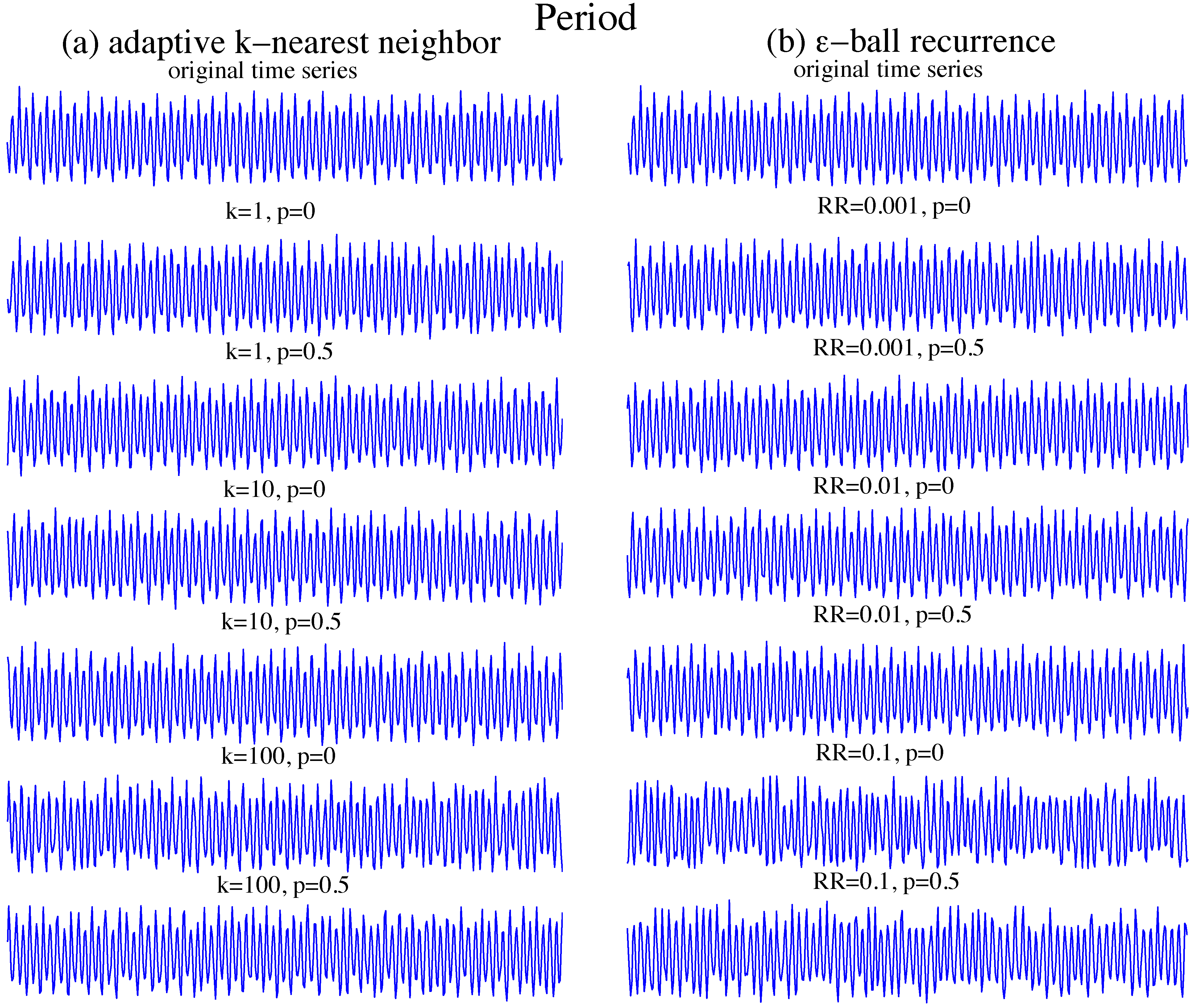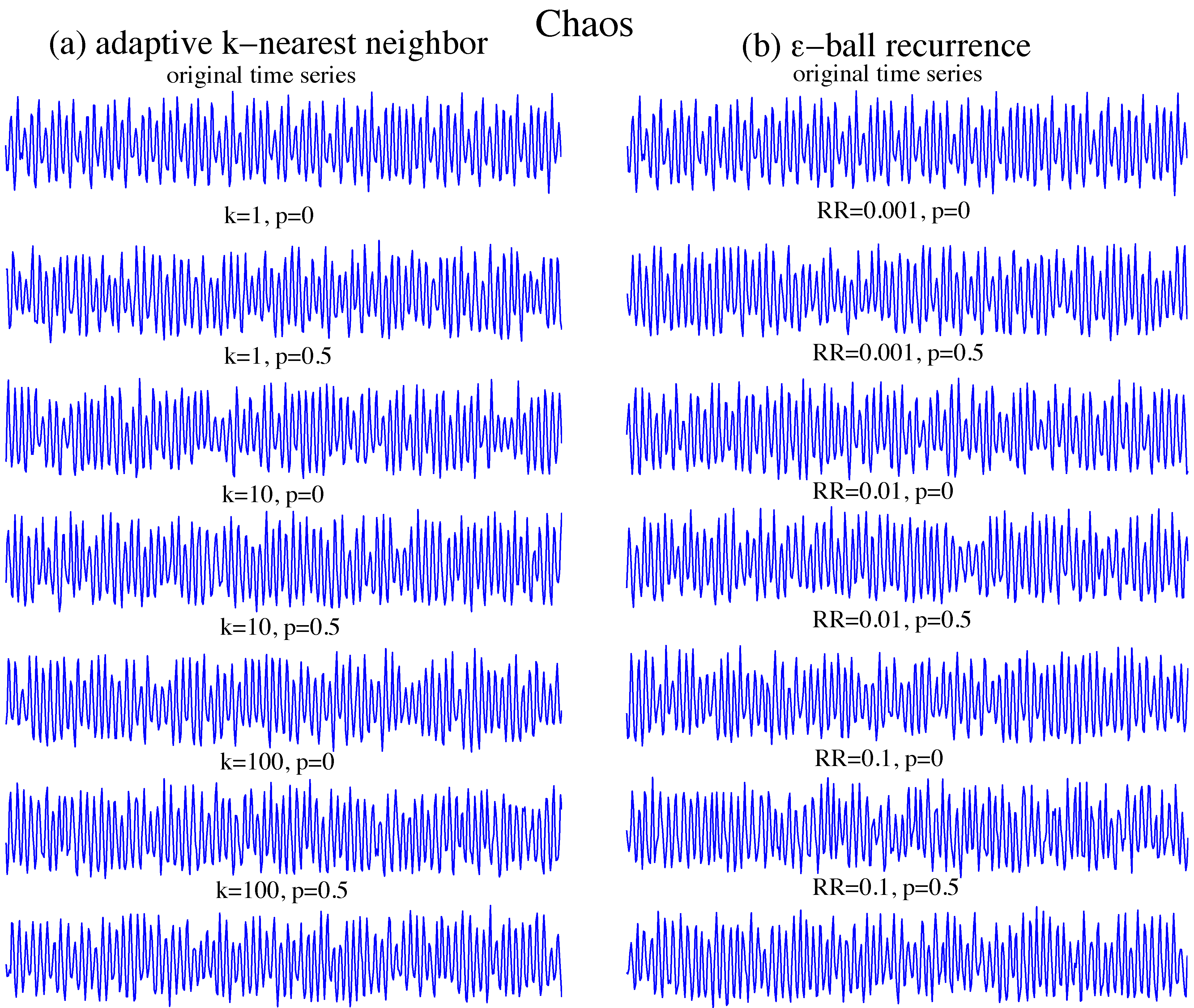The results are shown in Figure 1 for period-4dynamics and Figure 2 for chaos.

As shown in Figure 1 and Figure 2, the surrogates generated with $p=0.5$ are qualitatively closer to the original time series than with $p=0$. Moreover, the difference is most obvious when k or $RR$is large. This is because with $p=0.5$, it is easier to follow the original time series than when $p=0$. When k or $RR$ is small, for example $k=1$ or $RR=0.001$, the constructed networks are less highly connected. Therefore, the random walk algorithm could become trapped in one small connected part of the unconnected network when $p=0$, and then, the surrogates are no longer meaningful. In this case, there is no discernible difference as the local information in one small connected part is consistent with the globe information in the periodic time series.

Figure 1. Surrogates of the periodic time series of the Rössler system. (a) Surrogates from adaptive k-nearest neighbour networks; (b) surrogates from ϵ-ball recurrence networks. The original time series, top panels, is a noisy period-4 orbit. Going down the figure, we add increasing variability as recurrence rate ($RR$)(or k) increases, but also switch between unbiased neighbour selection ($p=0$) to bias towards selecting the node itself ($p=0.5$). With $p>0$, we see more reproducible short sections of trajectory between the data and surrogates. As k (or $RR$) increases, the simulations become more irregular. Beyond moderate values of randomisation (roughly $k=10$ or $RR=0.01$), the simulations generate behaviour qualitatively distinct from the original time series.

Figure 1. Surrogates of the periodic time series of the Rössler system. (a) Surrogates from adaptive k-nearest neighbour networks; (b) surrogates from ϵ-ball recurrence networks. The original time series, top panels, is a noisy period-4 orbit. Going down the figure, we add increasing variability as recurrence rate ($RR$)(or k) increases, but also switch between unbiased neighbour selection ($p=0$) to bias towards selecting the node itself ($p=0.5$). With $p>0$, we see more reproducible short sections of trajectory between the data and surrogates. As k (or $RR$) increases, the simulations become more irregular. Beyond moderate values of randomisation (roughly $k=10$ or $RR=0.01$), the simulations generate behaviour qualitatively distinct from the original time series.

Figure 2. Surrogates of the periodic time series of the Rössler system. (a) Surrogates from adaptive k-nearest neighbour networks; (b) surrogates from ϵ-ball recurrence networks. The original time series, top panels, is a noisy period-4 orbit. Going down the figure, we add increasing variability as $RR$ (or k) increases, but also switch between unbiased neighbour selection ($p=0$) to bias towards selecting the node itself ($p=0.5$). With $p>0$, we see more reproducible short sections of trajectory between the data and surrogates. As k (or $RR$) increases, the simulations becomes more irregular. For chaotic dynamics, the simulations appear more like the original time series for larger values of k and $RR$, particularly for the captive k-nearest neighbour method.

Figure 2. Surrogates of the periodic time series of the Rössler system. (a) Surrogates from adaptive k-nearest neighbour networks; (b) surrogates from ϵ-ball recurrence networks. The original time series, top panels, is a noisy period-4 orbit. Going down the figure, we add increasing variability as $RR$ (or k) increases, but also switch between unbiased neighbour selection ($p=0$) to bias towards selecting the node itself ($p=0.5$). With $p>0$, we see more reproducible short sections of trajectory between the data and surrogates. As k (or $RR$) increases, the simulations becomes more irregular. For chaotic dynamics, the simulations appear more like the original time series for larger values of k and $RR$, particularly for the captive k-nearest neighbour method.

From Figure 1 and Figure 2, we can see that the surrogates generated by adaptive k-nearest neighbour networks are more similar to the original time series than the ϵ-ball recurrence networks. Here, we focus on only one-connected networks, and we pay particular attention to surrogates generated by big k and $RR$. Taking the periodic surrogates with $RR=0.1$ for example, we can see that surrogates generated by ϵ-ball recurrence networks basically loose the underlying period. The fact that the surrogates generated by ϵ-ball recurrence networks with low $RR$ are better is somewhat surprising. For these surrogates, the corresponding networks have many nodes with no neighbours in the ϵ-ball recurrence networks, so the surrogates change to follow the original time series based on the supplementary rules of the random walk algorithm. In other words, it increases the probability p to follow the original time series. When $p=1$, we get exactly the original time series. Since the ϵ-ball recurrence method sets a fixed distance threshold, nodes in the denser part of the state space have more neighbours, and those in more sparsely populated areas, or on the boundary, have fewer neighbours (or even none). Therefore, we have to choose a bigger ϵ to ensure that the network is connected. However, such a large value of ϵ then gives some nodes too many neighbours, so that the next nodes of these nodes have too many possibilities. Therefore, the simulations will easily deviate from the original time series, which causes them to loose information, for example the periodic simulations with $RR=0.1$ in Figure 1.

3.2. Accurate Simulation and Good Models

By employing these networks to generate simulations of the original dynamical system, we are now treating the network as a model of the underlying system. The value of this model is in how well it is able to capture the salient features of the original system. To evaluate this, we can invoke the rationale of surrogate data analysis. The basic premise of surrogate data is to generate independent realisation of some dynamical system that are both qualitatively similar to the observed data (in particular ways, which we will come to in the next section) and also consistent with some particular model class. Here, the simulations are the realisation of the model class, and by treating them as surrogates, we can test how well that model is performing at capturing the important features of the underlying system.

Clearly, it is difficult to choose an appropriate ϵ to simultaneously meet both criteria. In contrast, the surrogates generated by the adaptive k-nearest neighbour networks seem both robust and stable. According to the method of adaptive k-nearest neighbour networks, we know that each node has at least k neighbours, which makes the networks more connected. As shown in Figure 1 and Figure 2, surrogates with $k=100$ and those with $k=10$ are very similar, so there are many appropriate k to choose. The fact that the k-neighbour approach applies an adaptive threshold to select nodes to be neighbours with an approximately constant rate is an advantage here, as it consequently ensures a flat invariant density. In the next section, we exploit this to generate a new form of surrogate time series.

4. Surrogates

In the field of nonlinear time series analysis, many different surrogate algorithms [31,32,33,34] have been proposed. Each of these algorithms is used to provide a robust statistical test of some specified null hypotheses. Theiler et al. [35] use the method of surrogate to identify nonlinearity in time series. The cycle shuffled surrogate approach [36] breaks the original time series into individual cycles and then shuffles these cycles; this tests for the presence of cyclic determinism. The null hypothesis is that the system is periodic, but otherwise, the dynamics are random. The alternative hypothesis is that there is inter-cycle deterministic dynamics evident in the data. Using continuous methods, Small et al. [37] proposed a simple pseudo-periodic surrogate method to test against the null hypothesis of a periodic orbit with uncorrelated noise; the method constructs (via an embedding process) the underlying dynamical system in phase space and then constructs a random walk according to the inferred dynamics.

In each case, the surrogate data algorithms proposed in the literature address a specific null hypothesis: they generate randomised data that are consistent with that hypothesis, but otherwise “like” the original data. In this case, the issue is a little more complicated. We can generate “surrogates” as realisations of random walks on the corresponding network. The null hypothesis is then that the network, and the inferred random dynamical system, is an adequate description of the underlying dynamics. Essentially, we are treating the network as a model of the dynamics and the surrogates as noisy simulations from that model. We are testing whether that model is a good model. There are two possible answers that we can arrive at: (1) the model simulations and the original data are indistinguishable, and therefore, the network is adequate for synthesising the dynamics of the underlying system; or (2) there are statistical discrepancies between model simulations and the original data. In the former case, we can employ the network (and simulations produced from this model) as adequate alternative samplings of the original dynamical system; this could be useful, for example, to provide parametric free estimates of the distribution of dynamical quantities, such as the correlation dimension or Lyapunov exponents. In the latter case, these discrepancies point to what is most interesting in the data and unable to be captured in the network.

Surrogate data must simultaneously appear qualitatively like the original data, while also conforming to the specific null hypothesis. Based on the comparison of the previous section, we select the method of adaptive k-nearest neighbours to construct the network and then execute the random walk algorithm on the constructed network to generate surrogates. Our comparison is based on one particular system, and we do not claim that this conclusion is universal. However, we have provided reasons why we expect this to be an appropriate conclusion in many situations.

The value of k (or, equivalently, $E_0$) is an important parameter, which needs to at least make the network connected. Although there is more freedom to choose a big k, we should avoid using too large values of k. The main reason is that too large k has more possibility to generate bad surrogates and to reduce the speed of computation of a feasible random walk. The other important parameter is the probability p in the random walk algorithm, which sensitively affects the deviation of surrogates from the original time series. The algorithm of surrogates is independent of the embedding parameter. We investigate some properties of surrogates as compared to the original time series.

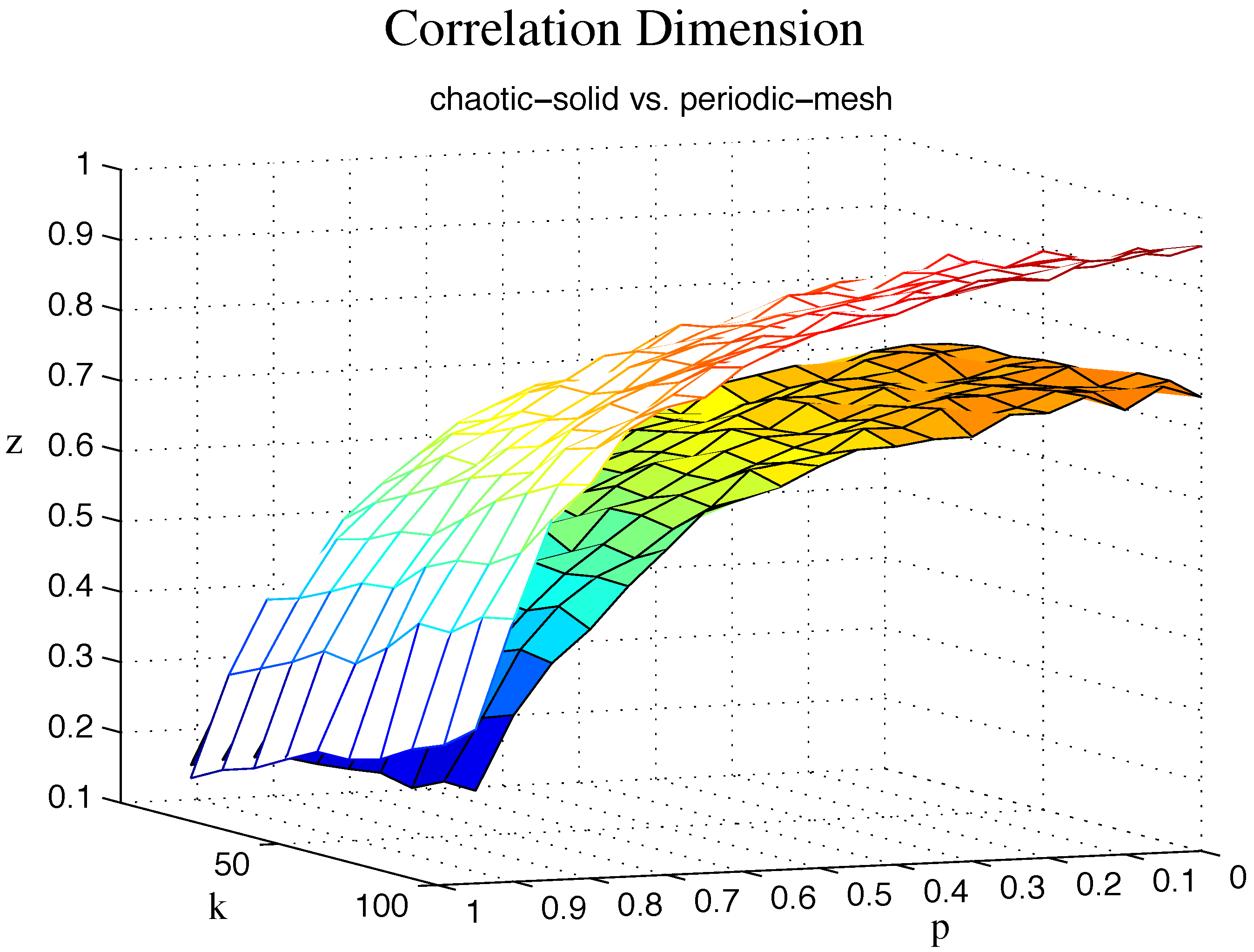
The correlation dimension was assessed using Grassberger and Procaccia’s [38,39] algorithm for the original time series and their surrogate time series. $D\left(r\right)$ is the number of pairs of points whose distance is less than a specified distance r. We use $max|D_s\left(r\right)-D_o\left(r\right)|$ to measure the discrimination between surrogate and original time series, where $D_o\left(r\right)$ is the number of original time series and $D_s\left(r\right)$ is that of the surrogate. As shown in Figure 3, the discrimination depends on the probability p, while the effect of neighbour parameter k is small. The discrimination of chaotic surrogates increases slowly as k becomes large. For the chaotic surrogates, the neighbour parameter k has no impact. Note, however, that upon computing the mean and standard deviation of the surrogate time series values for any particular values of k and p, we find that the true (original) system is within two standard deviations and, in most cases, within one standard deviation. That is, we cannot reject the null hypothesis, and these surrogate time series represent the output of a good model that is statistically indistinguishable from the data.

Figure 3. Comparison of the correlation dimension for surrogates. $z=log(max|D_s\left(r\right)-D_o\left(r\right)\left|\right)$ is used as the measure (the vertical axis). k is the parameter to construct an adaptive k-nearest neighbour network. p is the probability in the random walk algorithm. The chaotic and periodic surrogates are marked with solid and mesh, respectively.

Figure 3. Comparison of the correlation dimension for surrogates. $z=log(max|D_s\left(r\right)-D_o\left(r\right)\left|\right)$ is used as the measure (the vertical axis). k is the parameter to construct an adaptive k-nearest neighbour network. p is the probability in the random walk algorithm. The chaotic and periodic surrogates are marked with solid and mesh, respectively.

Figure 4. Comparison of the complexity for surrogates. $z=|C_s-C_o|$ is used as the measure (the vertical axis). k is the parameter to construct an adaptive k-nearest neighbour network. p is the probability in the random walk algorithm. The chaotic and periodic surrogates are marked with solid and mesh, respectively.

Figure 4. Comparison of the complexity for surrogates. $z=|C_s-C_o|$ is used as the measure (the vertical axis). k is the parameter to construct an adaptive k-nearest neighbour network. p is the probability in the random walk algorithm. The chaotic and periodic surrogates are marked with solid and mesh, respectively.

Lempel–Ziv complexity [40] has been widely used as a complexity measure for signal analysis; we introduce it here to compare complexity as a discriminating statistic for the surrogates and the original time series. $|C_s-C_o|$ is used to measure the complexity difference between surrogates and original time series, where $C_s$ represents the complexity of surrogates and $C_o$ is that of the original time series. It is obvious that the complexity difference between surrogates and original time series in chaotic systems is bigger than that in periodic systems; see Figure 4. Again, for both systems, complexity discrimination is dependent on the probability p. Additionally, the discrimination increases slowly as k becomes large, which is clearer when p is small. However, just as with the correlation dimension, the differences between data and surrogates are within two standard deviations of the mean.

In each case, results for the surrogates are within (usually, well within) two standard deviations of the mean for the data. While in the figures, we report absolute deviation, our calculations show that the deviation is not statistically significant. In each case, the surrogates produce realisations for which the algorithmic complexity or correlation dimension is statistically indistinguishable from the data.

5. Conclusions

In this paper, we discussed the existing approaches to construct complex networks from time series and a proposed random walk algorithm to invert the process and generate independent simulations from the same complex network model: nonlinear network-based surrogates. The methods of adaptive k-nearest neighbour and ϵ-ball recurrence are explained in detail and are compared to the random walk algorithm. We see that when employed to reconstruct the dynamics from the network, the adaptive k-nearest neighbour algorithm for generating networks out-performs methods based on ϵ-ball recurrence. This indicates that the adaptive k-nearest neighbour algorithm preserves dynamical properties of the original system more faithfully than ϵ-ball recurrence. The experiment results also show that the adaptive k-nearest neighbour network is better by comparing the surrogates. Using the adaptive k-nearest neighbour networks, we analyse the effects of the parameters on the surrogates and give some advice to choose the suitable parameters. In all cases, empirical choices, based in our previous experiences, were sufficient to obtain optimal parameter choices. We find that probability p needs to be moderate and neighbourhood size k only large enough to capture the dynamics.

Nonetheless, when we quantify the dynamical discrepancy between the original data and an ensemble of surrogates (using either algorithmic complexity or correlation dimension), we see very good agreement for all systems over a wide range of scales. Hence, the inversion process, from network back to time series, is generating time series that are a good representation of the underlying dynamics of the dynamical system. That is, these networks act as an accurate and sufficient model of the deterministic dynamics.