1. Introduction
Determining an entropy of random variable has been broadly studied since the nineteenth century. Originally, the entropy concept crystallized in thermodynamics and quantum mechanics [
1,
2]. In information theory, the entropy was introduced by Claude Shannon [
3] in 1948 for random variables with a discrete probability space. A natural extension of a discrete entropy is a differential entropy [
4] defined for a continuous random variable with probability density function (pdf)
by:
It is worth mentioning that both notions, although analogous, have different properties, e.g., differential entropy is not necessarily non-negative.
The notion of entropy has many applications in various research fields. As an example, we mention here the emerging field of systems biology. It combines knowledge from various disciplines, including molecular biology, engineering, mathematics and physics, to model and analyze cellular processes. One of the challenging tasks in systems biology is to study interactions of regulatory, signaling and metabolism processes by means of biochemical kinetic models [
5]. To check the robustness of such models, adequate sensitivity analysis procedures have to be applied.
Efficient entropy estimation is crucial for sensitivity analysis methods based on the mutual information of random variable measurements. An interesting approach for multi-variables system has been proposed recently by Lüdtke
et al. [
6]. However, it is based on a discrete entropy estimator and requires a computationally-inefficient variable discretization procedure. Having this concerns in mind, we propose here a more efficient
k-
nn differential entropy estimator, which can be used to calculate sensitivity indices in lieu of its discrete equivalent. Its application to sensitivity analysis for the model of the p53-Mdm2 feedback loop is presented in
Section 5. In our approach, there is no need for variable discretization, and more importantly, an improved entropy estimator can be successfully used for highly multidimensional variables.
The estimation of differential entropy from the sample is an important problem with many applications; consequently, many methods have been proposed. Furthermore, several estimators based on the
k-
nn approach were analyzed, and their mathematical properties were investigated; see the discussion in the next section. We would like to emphasize that our main motivation here was very practical. Therefore, we focused on efficient implementation and bias correction for the well-established
k-
nn estimator with already proven consistency. The theory justifying our bias correction algorithm is based on the consistency analysis by Kozachnko and Leonenko [
7]. Moreover, we performed extensive simulations for random samples from many multidimensional distributions recognized as most adequate in systems biology models.
Our improved
k-
nn entropy estimator explores the idea of correcting the density function evaluation near the boundary of random variable support. This smart idea has been proposed previously in [
8] for several distributions. However, the novelty and usefulness of our approach lies in efficient bias correction of the classical
k-
nn estimator, which is applicable for any data sample (
i.e., the
a priori knowledge of the underlying distribution is not required).
2. k-nn Estimators of Differential Entropy
There are several approaches to entropy estimation from data samples; some are based on random variable discretization by partitioning [
9], while others aim to estimate the probability mass according to the pdf [
8,
10]. The most efficient methods for probability mass estimation are based on k-th nearest neighbor (
k-
nn) estimation. The first
k-
nn approach to entropy estimation is dated to 1987 with the entropy estimator provided by Kozachenko and Leonenko [
7] together with the proof of convergence. In this section, we recall definition and main properties of the
k-
nn entropy estimator by Kozachenko and Leonenko and we compare it to other approaches proposed in the literature.
Denote by
for
i.i.d. samples of continuous random variable
. Let
be the
d-dimensional distance of point
to its nearest neighbor in the sample and
be the volume of a
d-dimensional unit ball. The estimator is defined for
d-dimensional distributions as follows [
7]:
white where
is the Euler–Mascheroni constant.
For completeness, we recall here the further study conducted by Kraskov
et al. [
11], who proposed a variant of the entropy estimator for the k-th nearest neighbor:
where
is the
d-dimensional distance of point
to its k-th nearest neighbor in the sample and
is the digamma function with
and
.
Notice that for , the Kraskov estimator given by Equation (2) performs almost equally to the Kozachenko–Leonenko estimator defined in Equation (1) with only a small unnoticeable difference stemming from:
According to analyses presented by Kozachenko
et al. (1987) and Kraskov
et al. (2004) in [
7,
11],
k-
nn estimators defined by Equations (1) and (2) converge in probability towards the real entropy value with increasing sample size:
Both estimators were shown to be consistent,
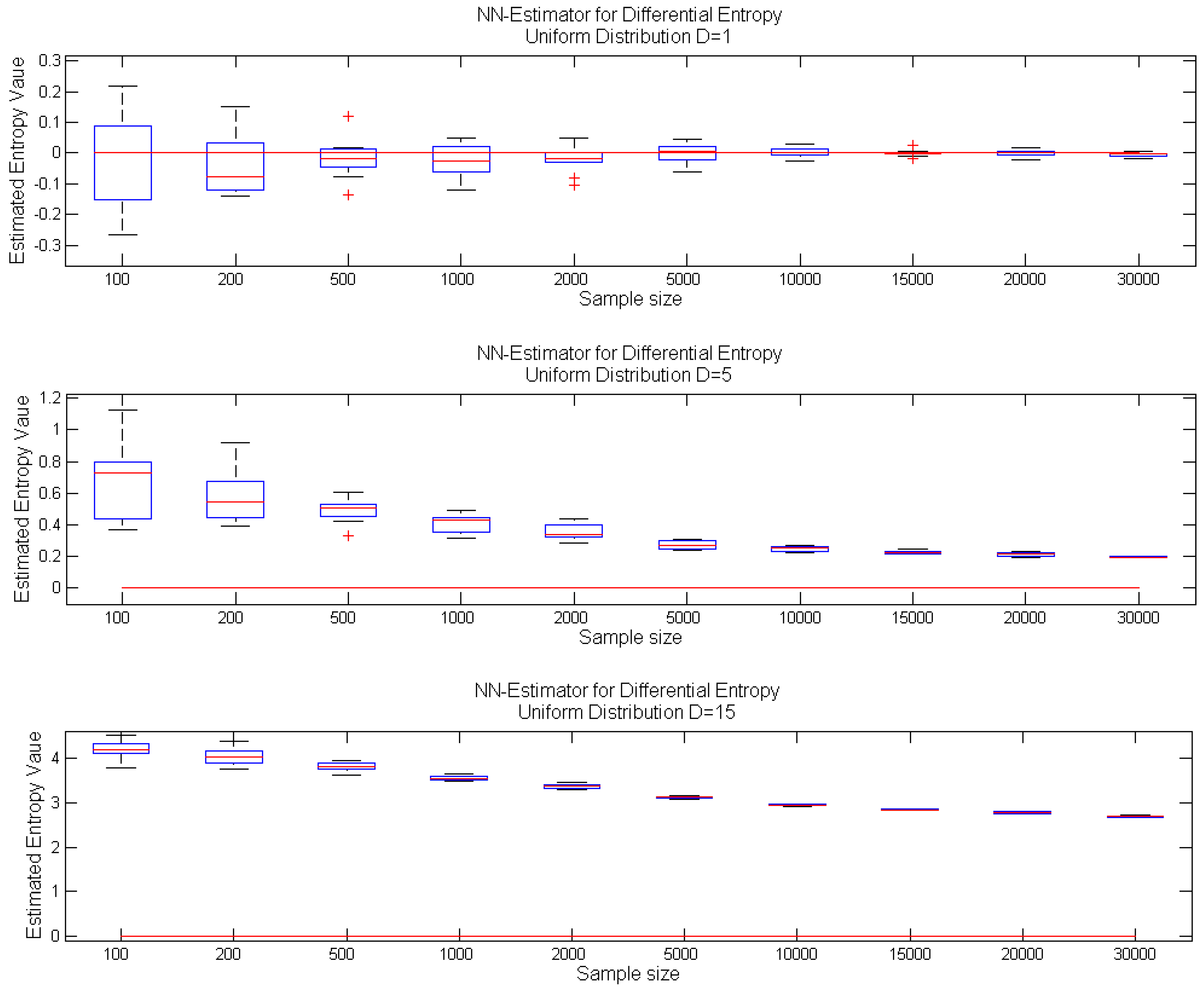
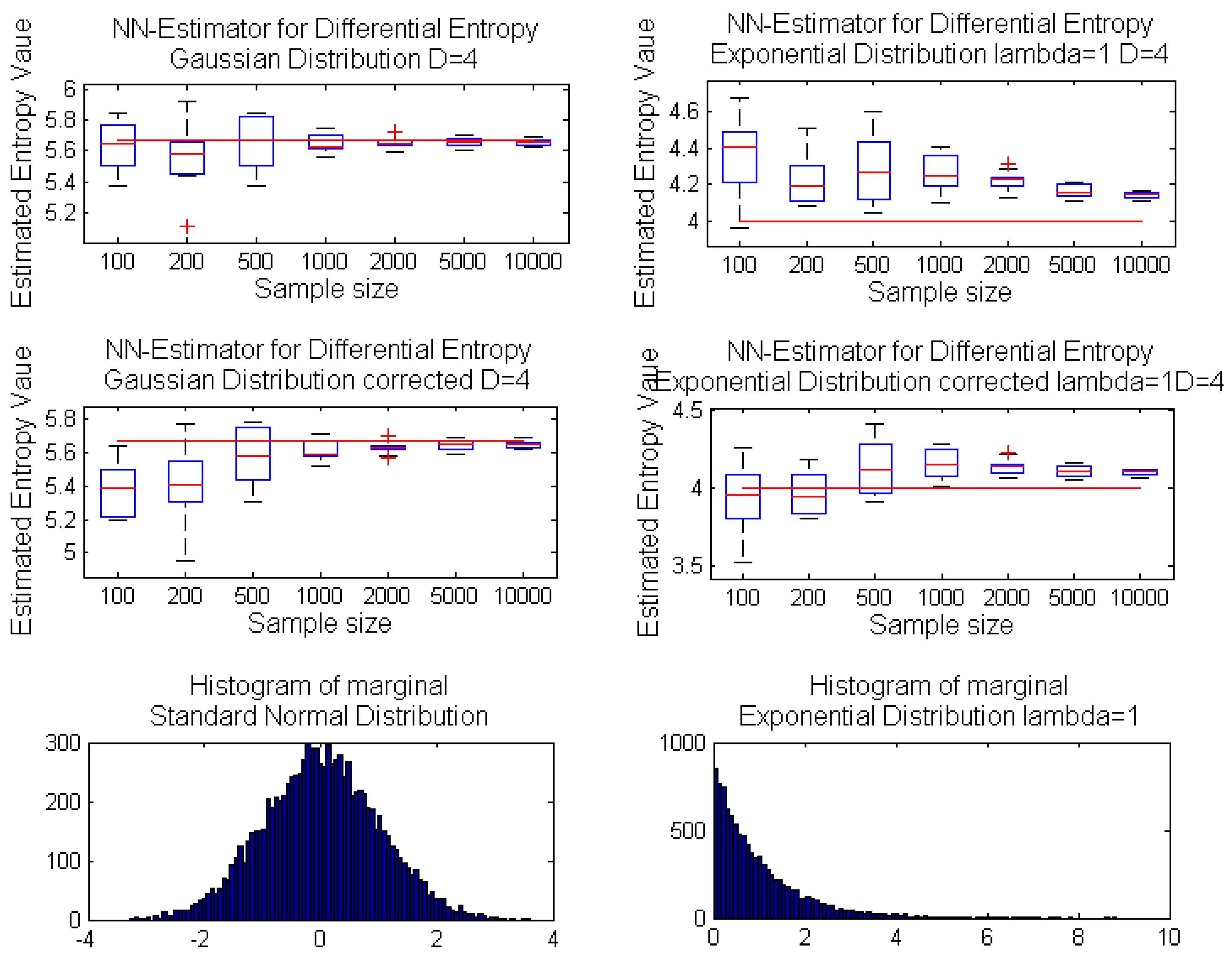
i.e., asymptotically unbiased with the variance vanishing as the sample size increases. Moreover, for one-dimensional random variables, the estimator can be considered unbiased, even for a relatively small sample size, whereas the increase of dimension results in significant estimator bias even for a moderate sample size; see the exemplary case in
Figure 1. The proof presented in [
7] of the Kozachenko–Leonenko estimator in Equation (1) requires the following condition on the pdf
for the asymptotic unbiasedness of the estimator:
and for the estimator consistency:
where
denote a metric in
and the expectations are over independent variables
x and
y.
Figure 1.
Performance of the k-nn estimator Equation (1) for increasing sample size: box-plots of estimated entropy values for samples from a uniform distribution: on interval [0,1] (top); on hypercube (center); on hypercube (bottom); with real entropy value denoted by the red line.
Figure 1.
Performance of the k-nn estimator Equation (1) for increasing sample size: box-plots of estimated entropy values for samples from a uniform distribution: on interval [0,1] (top); on hypercube (center); on hypercube (bottom); with real entropy value denoted by the red line.
Pérez-Cruz (2008) in [
12] requires a somehow weaker assumption that the pdf must exist,
i.e., the probability measure must be absolutely continuous. Consequently, the almost sure convergence of the entropy estimator
is stated by the author.
The
k-
nn estimator for the related notion of Shannon entropy was proposed by Leonenko
et al. (2008) in [
13]. It can be shown that it is equivalent to those defined by Equation (2) with component
replaced by
. Similarly, the Shannon entropy estimator presented by Penrose
et al. (2013) in [
14] can be expressed by Equation (1) with the component
replaced by
. Both estimators were proven to be convergent to the real entropy value in
with some restrictions for density
. Namely, in [
13], the pdf must be bounded, and
for some
. The boundness condition has been relaxed in [
15] to an unbounded pdf with additional constraint
; white while in [
14], the pdf must be bounded or the pdf must be defined on
with
It is worth mentioning that also, estimators for the Kullback–Leibler divergence were proposed and analyzed by Pérez-Cruz and Wang in [
12,
16]. Nevertheless, these estimators were based on the same idea of probability mass estimation by the distance to the
k-
nn in a sample; consequently, when used for estimating mutual information (
cf. Definition 2), they suffer from the same problems as the above-mentioned entropy estimators.
A slightly different concept based on order statistics generalized to Voronoi regions in multiple dimensions was explored by Miller [
17] to estimate the differential entropy and applied in [
18] for independent component analysis. Unfortunately, the complexity of calculating the volume of Voronoi regions appears to be exponential in the dimension, and therefore, the method does not seem to be promising for our applications.
3. Bias Correction of the k-nn Entropy Estimator
In higher dimensions,
k-
nn estimators for many important distributions converge slowly and with noticeable bias;
cf. Figure 1. Moreover, the entropy value is often overestimated; see
Figure 1 for a
d-dimensional uniform distribution and
Appendix Figure A1 for a
d-dimensional distribution with independent marginals sampled from an exponential distribution. On the other hand, for some distributions, like multivariate Gaussian ones, the estimator performs well, even in higher dimensions;
cf. Appendix Figure A1 (top panel). As argued in [
8], the overestimation problem affects random variables with bounded support. Before giving the description of our bias correction procedure, we briefly present the density mass estimation problem.
Recall that the k-nn estimation for continuous random variables requires probability mass estimation in small neighborhoods of sampled points. Consequently, when the sample points are located densely near the boundary of a given distribution, the calculations might be overestimated, as the samples’ neighborhoods might exceed the boundary of random variable support.
Therefore, the entropy estimator bias stems from overestimation of the pdf that occurs when the sample point is located near the boundaries of a random variable support. The curse of dimensionality implies that the boundary area increases with the variable dimension. Thus, in higher dimensions, neighborhoods of sampled points more frequently exceed the boundaries of a variable support.
Here, we focus on correcting the bias of the
k-
nn estimator. We restrict our further analysis to the Kozachenko and Leonenko estimator in Equation (1), but our procedure may be easily adapted to reduce the bias of the estimator defined by Equation (2) and other estimators discussed in the previous section. The precise reason for the biased performance of the
k-
nn entropy estimator may be exposed by analyzing the proof of its convergence [
7].
Let
be a set of independent random samples of a variable
with probability density function
. Let
be a metric in
with a neighborhood of radius
r centered at point
x defined by:
Then, the volume of the neighborhood is equal to
, where
is the unit ball volume according to the metric
ρ.
For differential entropy estimation, the probability mass of a random variable X in a point is estimated using the following Lebesgue theorem with a small volume neighborhoods centered at sampled points .
Theorem 1 (Lebesgue)
. Let ; then, for almost all and open balls with radius : By analyzing the proof of convergence of the
k-
nn estimator (see the
Appendix), we noticed that the application of Lebesgue’s theorem for distributions with support
can introduce a systematic error to the estimated value. The formal analysis reduces to a quotation of the main steps of the proof of convergence. The key point of the proof in which the systematic error is to be noticed is presented in Equation (B1) in the
Appendix. The bias stems from the relatively slow convergence with the sample size to the exponent of the averaged pdf within neighborhoods of vanishing volumes that can exceed variable support.
To illustrate this issue, let us consider the exemplary case of the uniform distribution
X on
d-dimensional unit cube
. Every point in a cube is equally probable and the pdf
for points
and
for points
outside the the cube. Lebesgue’s theorem applied for
X states:
and it introduces the following estimation error for points
x near the boundaries,
i.e., with neighborhood
partially outside the cube
:
where
. Our correction to the entropy estimator is based on the logarithm of the proportions of neighborhood volumes
inside the support of
X to the volume of the whole neighborhood
:
Finally, for
defined by Equation (1), the corrected entropy estimator is defined as follows:
To ensure the efficient implementation of our approach, we use the maximum metric in
:
for points
and
. In this metric, the neighborhoods are
d-dimensional hypercubes, and the unit ball volume equals
.
The support boundaries are estimated based on the sample and are determined simply as the leftmost and the rightmost values for each dimension. Determined boundary values (in an amount of at most ) are removed from the sample in the preprocessing phase, before entropy estimation.
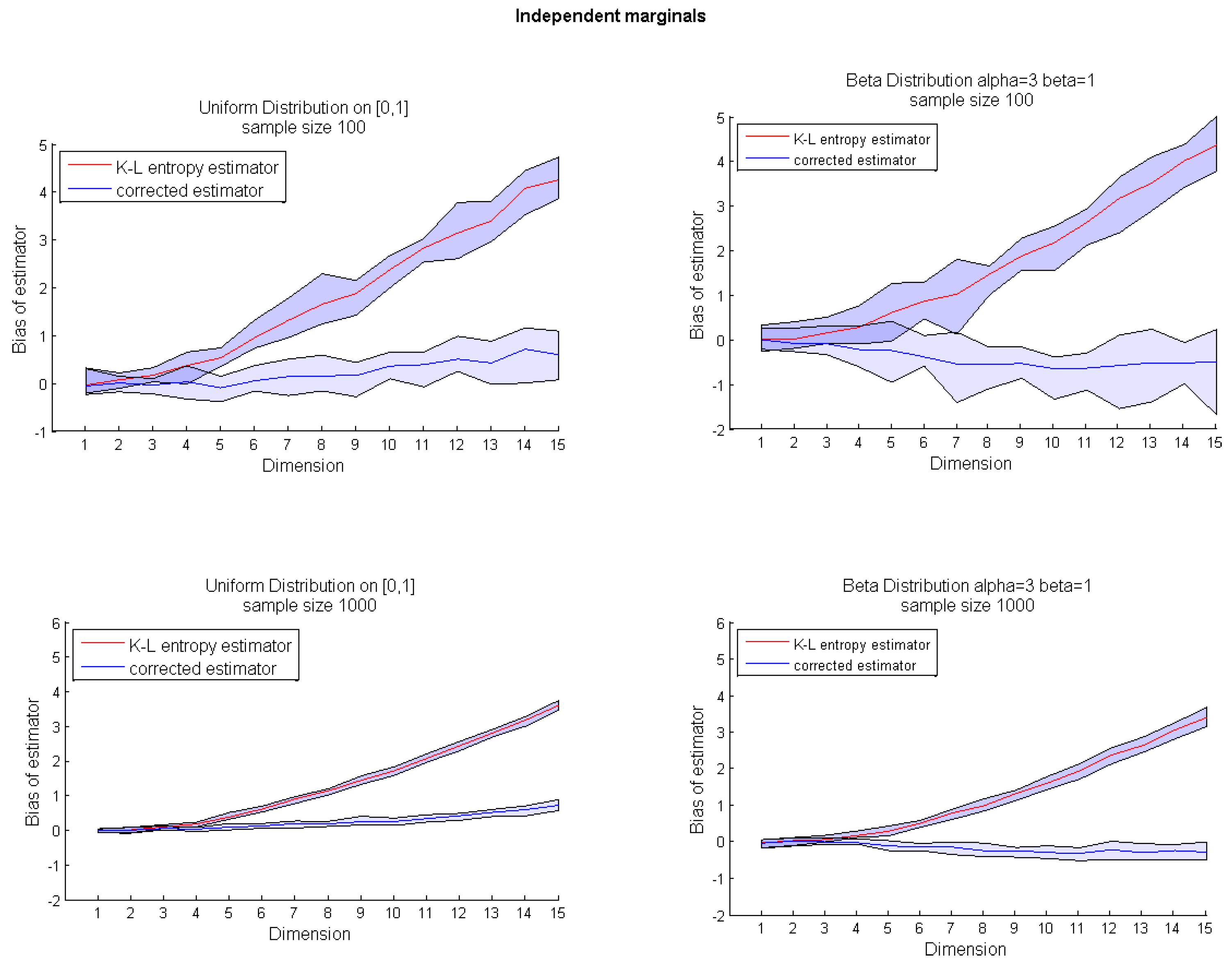
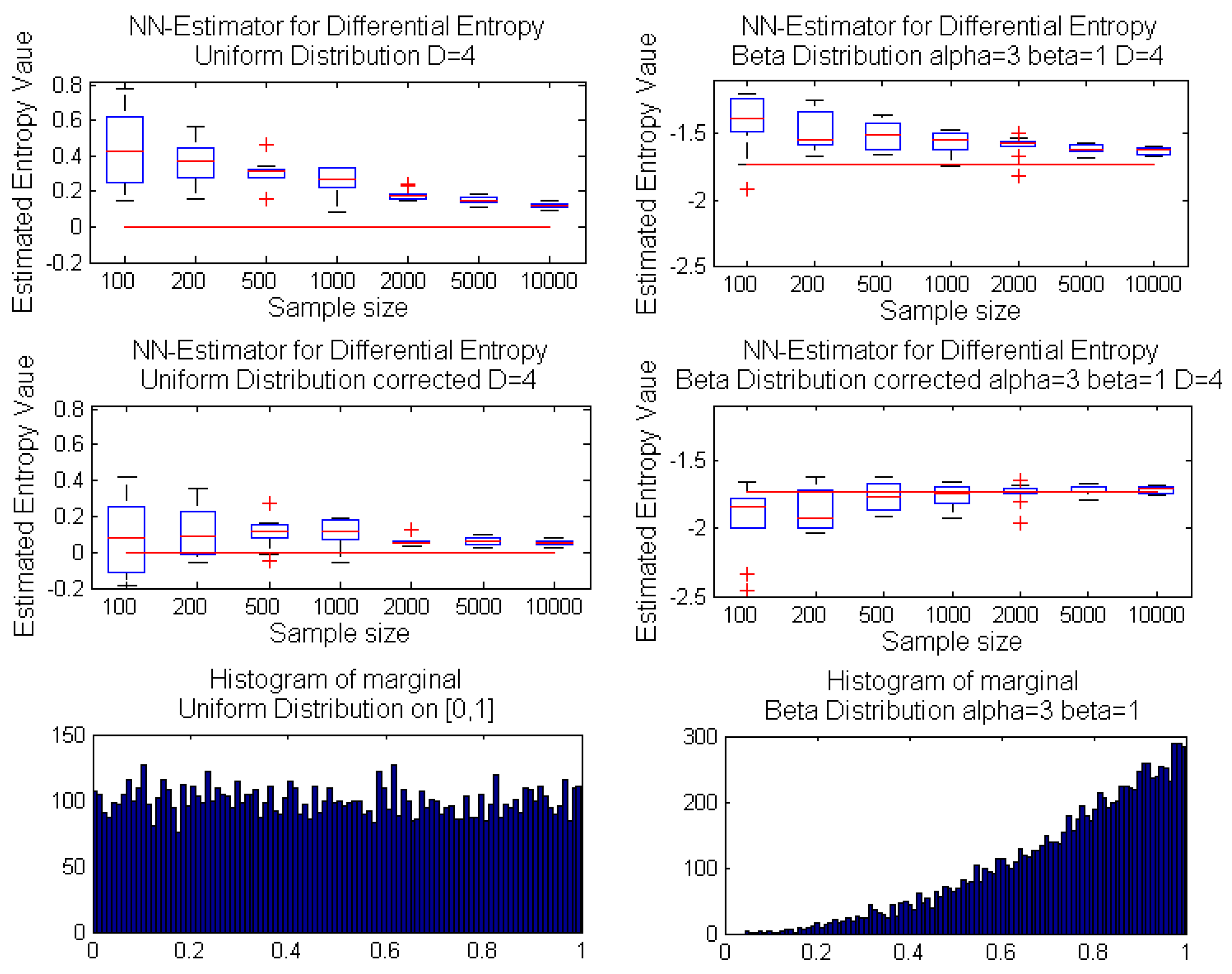
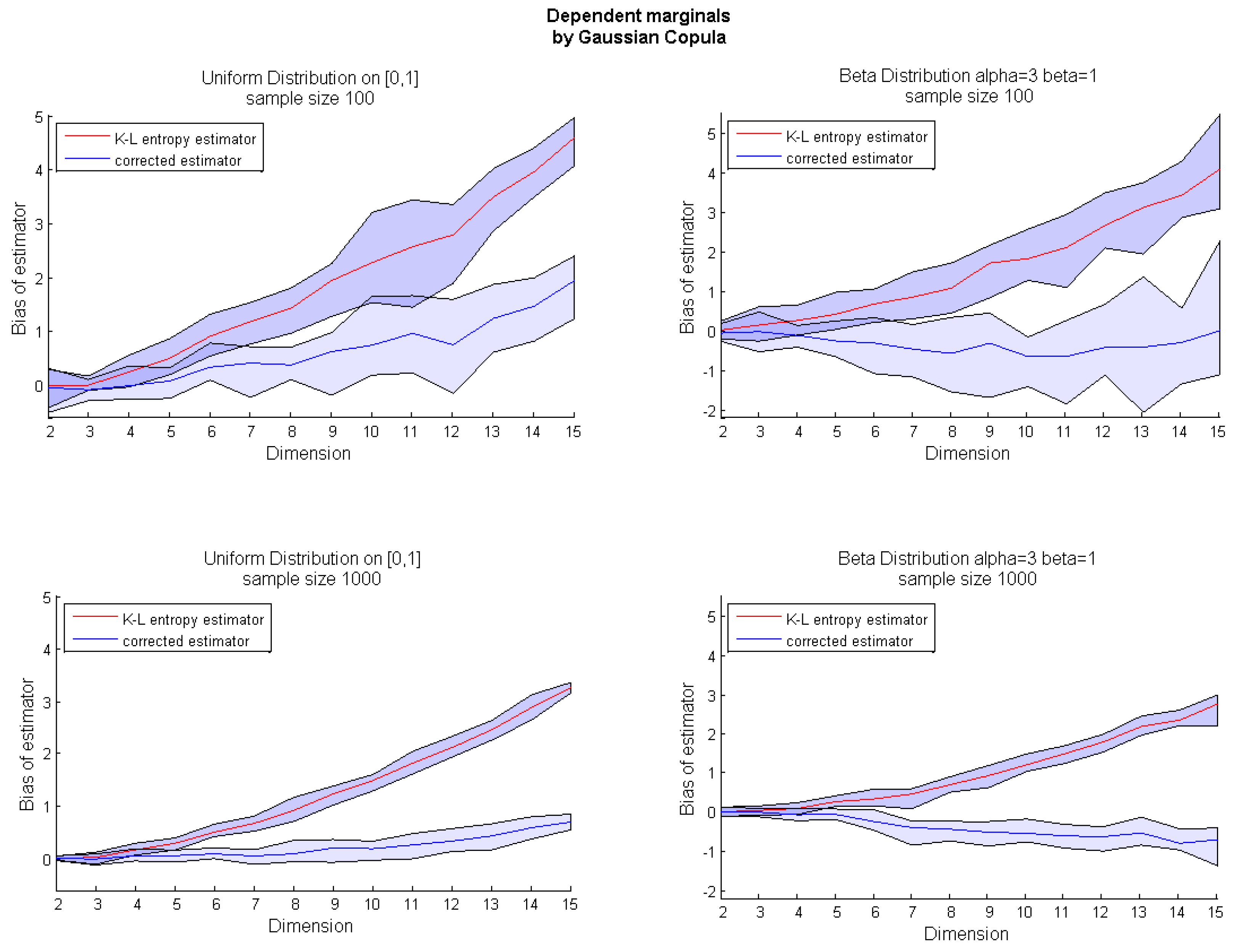
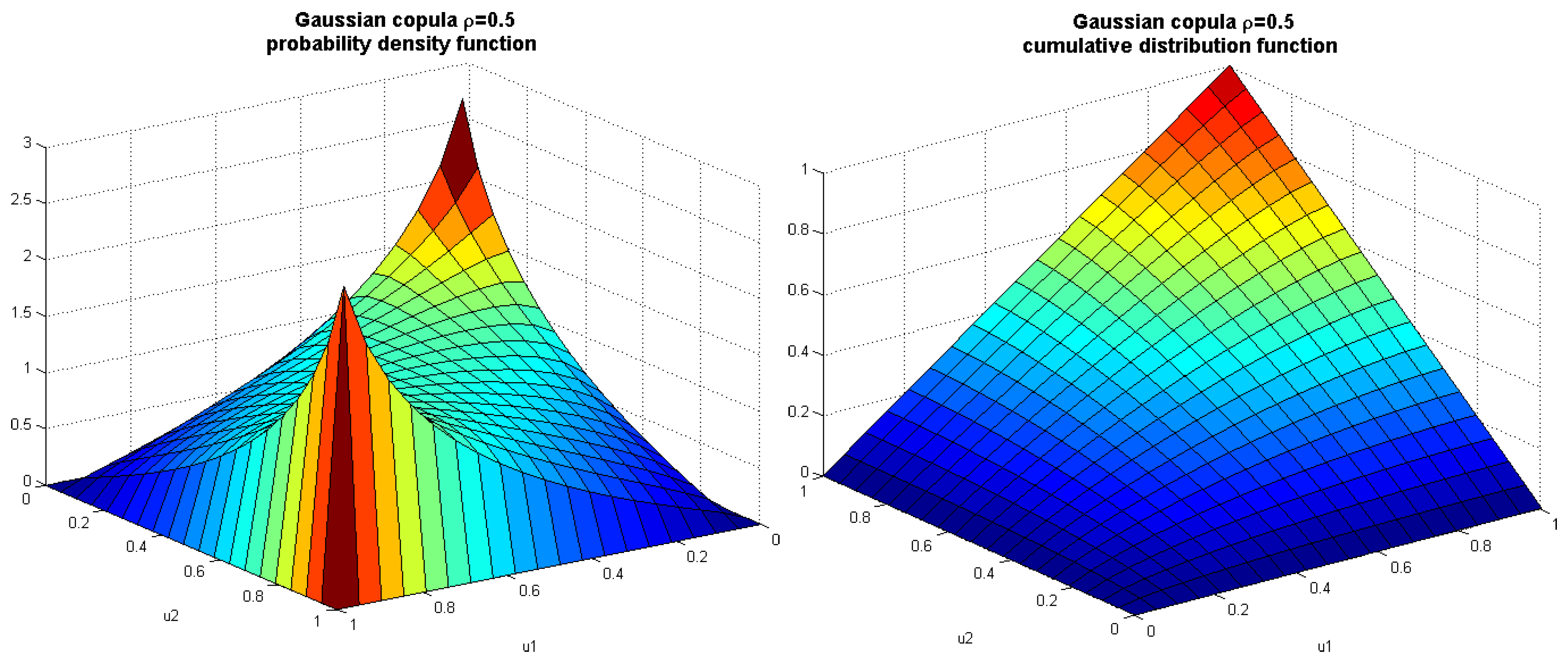
Algorithm 1 presents the pseudocode of the corrected k-nn entropy estimator. The bias correction presented on the uniform example can be applied for any multivariate distribution. However, due to the source of bias, our correction is much more efficient for random variables with bounded support. Therefore, in the next section, we focus on the usefulness of Algorithm 1 for multidimensional uniform and beta distributions with both independent and dependent marginals. The exemplary dependency structure is modeled by a Gaussian copula.
The issue of estimator convergence for a one-dimensional variable has been analyzed by van der Meulen and Tsybakov [
19], and the bias was proven to be of order
, where
n is the sample size.
Furthermore, the bounded support of a random variable as a source of
k-
nn estimator bias was already identified in papers by Sricharan
et al. [
8,
20]. The authors estimated the bias using Taylor expansion of pdf
, as:
where
, under the assumption that
p is two-times continuously differentiable and is bounded away from zero. Compare also further work by Sricharan
et al. [
21,
22].
It should be emphasized that the usefulness of analytical bias estimations is limited to variables with known pdf
. In contrast to previous approaches, we did not aim at proving asymptotic bounds for differential entropy estimator bias. Instead, we propose the efficient heuristic procedure for bias correction. Moreover, in the applications, e.g., in systems biology, we have no
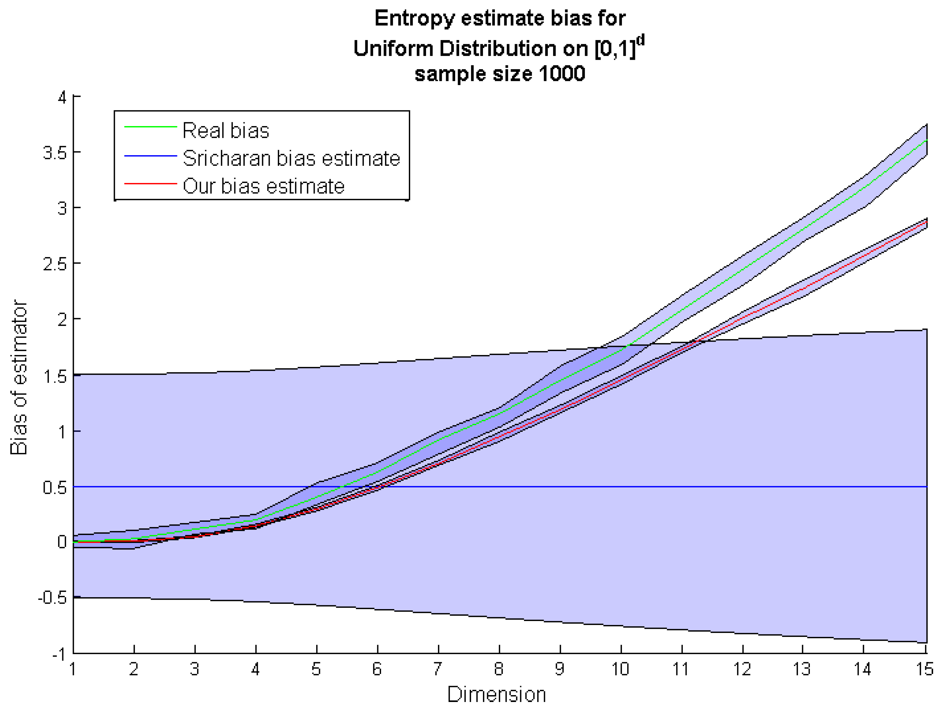
a priori knowledge about the probability distributions of a random sample. The analytical bounds as in Equation (7) is of limited value without knowledge of pdf. To compare our bias correction procedure (Algorithm 1) to the estimation given by Equation (7), we calculated both corrections for a d-dimensional uniform distribution (see
Figure 2). It occurred that compared to our method , the Equation (7) significantly underestimates the bias for higher dimensions.
Figure 2.
Comparison of the
k-
nn entropy bias estimate by Sricharan
et al. [
8] (blue line) with the real bias based on the
k-
nn entropy estimation from sampled points (green line) and the
k-
nn entropy bias estimate obtained by our method (red line).
Figure 2.
Comparison of the
k-
nn entropy bias estimate by Sricharan
et al. [
8] (blue line) with the real bias based on the
k-
nn entropy estimation from sampled points (green line) and the
k-
nn entropy bias estimate obtained by our method (red line).
5. Sensitivity Indices Based on the k-nn Entropy Estimator
Efficient entropy estimation is crucial in many applications, especially in sensitivity analysis based on mutual information [
6]. Particularly, in systems biology, aiming to formally describe complex natural phenomena, an in-depth sensitivity analysis is required to better understand the modeled system behavior. Although, the method proposed by Lüdtke
et al. [
6] provides an approach to sensitivity analysis for multi-variables system, it is based on entropy estimation requiring variable discretization and, consequently is computationally inefficient. Moreover, it may provide biased or inadequate results for continuous random variables.
Therefore, here, we propose to modify the approach from [
6] by applying our corrected
k-
nn differential entropy estimation with no need for variable discretization. The main concept in sensitivity analysis, taken from information theory, is mutual information (MI) between random variables. Mutual information indicates the amount of shared information between two random variables,
i.e., input variable (parameter or explanatory variable) and output variable (explained variable). When used for samples of parameters and samples of corresponding model response, estimated MI can indicate the sensitivity of a model to the parameters.
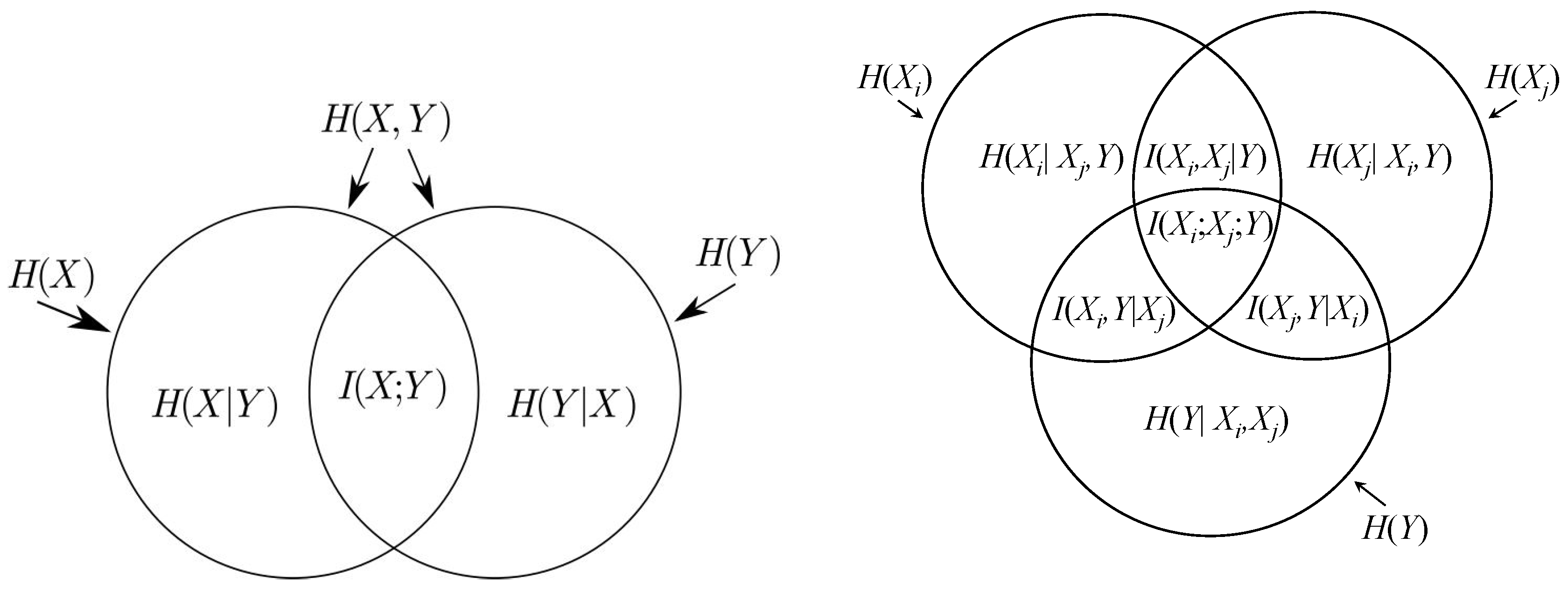
Definition 2. The mutual information between continuous random variables and is defined by:where is the joint distribution of X and Y and , and are probability density functions. Definition 3. The conditional entropy of a random variable given random variable is defined as:where and are respectively the joint and the conditional probabilities densities functions of variables X and Y. There exist the following analogies between the information theoretic measures and set theory operations (see
Figure B1 in the
Appendix):
| information theory | set theory |
| |
| |
| |
Inspired by [
6], we redefine sensitivity indices for parameters (considered as continuous random variables) using the notion of differential entropy:
Definition 4. white Assume that are the parameters of the model and Y is the model output, then single sensitivity indices are defined as: white Analogously, group sensitivity indices for pairs of parameters are defined as:
Clearly, Definition 4 can be extended for any subset of parameters.
The sensitivity indices reflect the impact of parameters on the model output. It may happen that the group sensitivity index for a pair of parameters had a high value, indicating the significant influence of these parameters, while two single sensitivity indices for these two parameters had a low value. We interpret such a case as the opposite (negative) interaction between this pair of parameters. To quantify such interactions, we use the following notion:
Definition 5. If are parameters of the model and Y is model output, then interactions indices within a pair of parameters are defined by: An analogous definition of interactions was introduced by McGill in [
24] for discrete random variables. The following corollary expresses the interaction indices by the group sensitivity indices; see also the Venn diagrams depicted in
Figure B1 in the
Appendix.
Corollary 6. Interaction index within the pair of parameters and can be expressed as the sum of single sensitivity indices of parameter and parameter to the output variable Y minus the group sensitivity index for a pair of parameters: 5.1. Case Study: Model of the p53-Mdm2 Feedback Loop
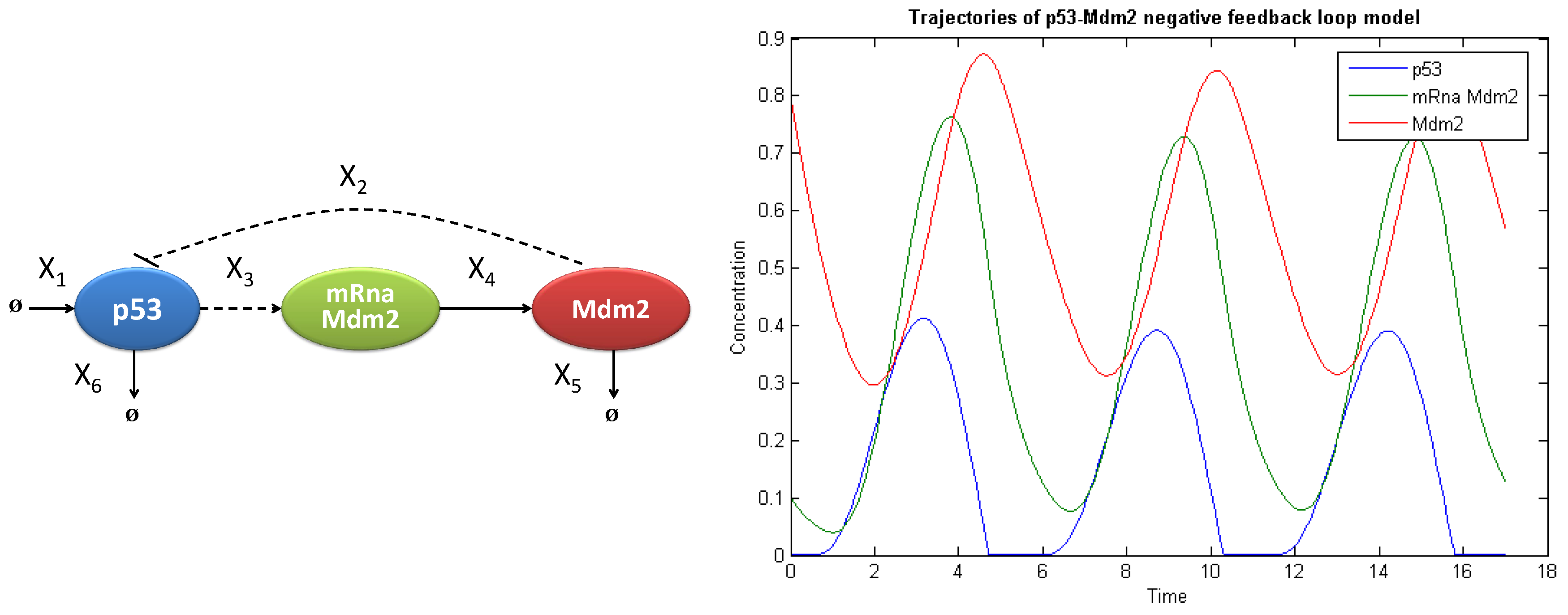
To validate the new approach to the global sensitivity analysis based on the entropy measure, we tested the method on a well-known and widely-studied example of the negative feedback loop of the p53 protein and Mdm2 ligase.
Tumor suppressor p53 protein, also known as TP53 transcription protein 53, is a transcription factor determining the fate of a cell in the case of DNA damage; p53 indirectly, via activation of the transcription of the encoding p21 gene, can block the cell cycle to repair DNA or activate a process of programmed cell death, called apoptosis. The main regulator of the concentration of p53 protein is ligase Mdm2/Hdm2 (double minute 2 mouse/human double minute 2), which, through ubiquitination, leads to degradation of p53 in the proteasome. In more than half of the cases of human cancers, p53 is inactivated or absent, which allows the mutated tumor cells to replicate and determines their immortality. Consequently, this protein is under investigation due to its property of leading to self-destruction of cancer cells, which could be successfully used as therapy in many types of cancer [
25]. The modelled system (
Figure 7 left panel) can be formally described with the use of ordinary differential equations (ODE) as follows:
where the variables of the modeled system
correspond to the concentration of species p53, mRna Mdm2 and Mdm2, respectively. The initial values of the variables are given by species concentrations at starting time point
:
| p53 protein; |
| Mdm2 ligase; |
| mRna Mdm2 precursor of Mdm2 ligase. |
The parameters of the model denoted by
correspond to reaction rates with the following base values
and their biological interpretations:
| p53 production; | | Mdm2 transcription; |
| Mdm2-dependent p53 degradation; | | Mdm2 degradation; |
| p53-dependent Mdm2 production; | | independent p53 degradation; |
| p53 threshold for degradation by Mdm2. | | |
To investigate the sensitivity of the model to the parameter changes, the parameters (
) were perturbed around the base value
according to Gamma distributions:
with shape parameters
and
and mean values equal to parameter base values
. The negative regulation of p53 protein by Mdm2 ligase results in an oscillatory behavior in time (see
Figure 7 right panel). A parameter responsible for negative regulation is Mdm2-dependent p53 degradation rate denoted by
.
Figure 7.
Graphical scheme of the modelled system (left); and the oscillatory behavior for the considered parameters values (right).
Figure 7.
Graphical scheme of the modelled system (left); and the oscillatory behavior for the considered parameters values (right).
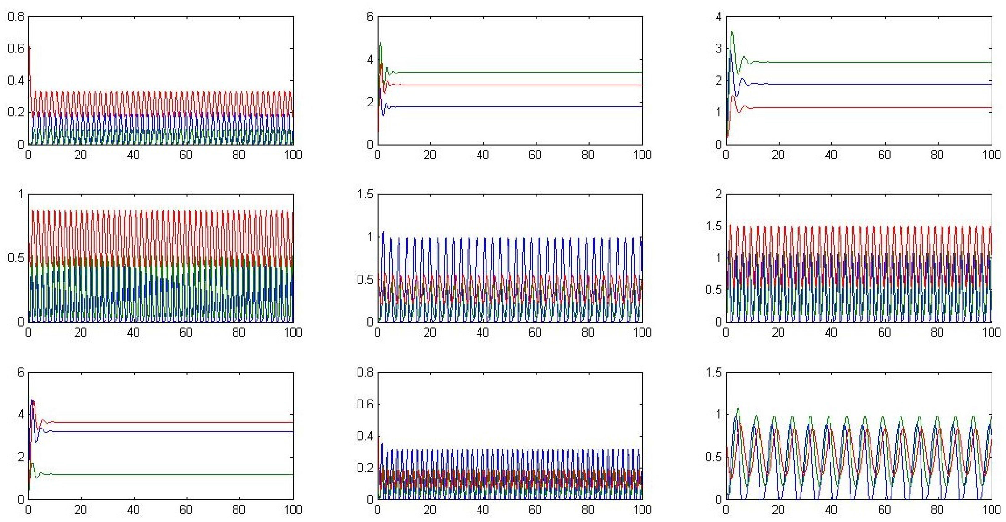
Different possible system trajectories resulting from the perturbation of parameters are depicted in
Figure B2 in the
Appendix. It is worth noting that oscillatory behavior is sensitive to specific parameter values.
The output of the model
Y is a three-dimensional variable with components denoting the species concentration that are averaged with respect to time:
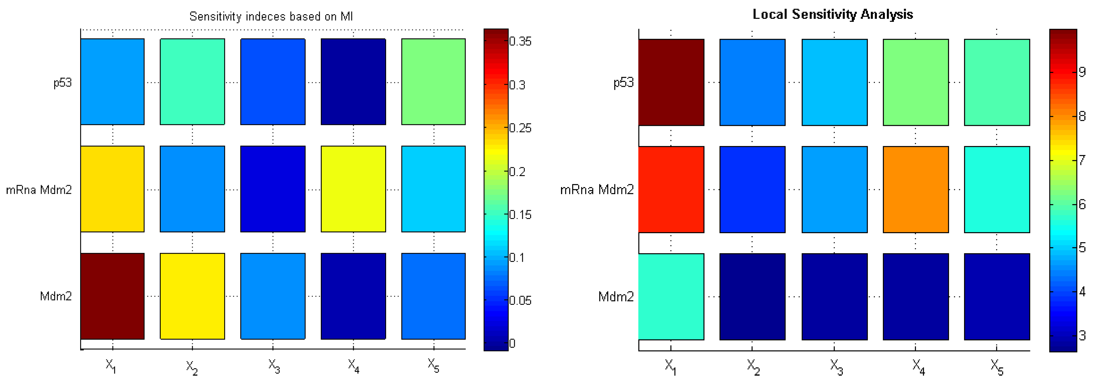
To interpret novel sensitivity indices based on differential entropy, we compared them to standard local sensitivity indices, which are partial derivatives of model output w.r.t. the parameters of interest. As illustrated by the heat maps in
Figure 8, both methods indicated the model inflow and outflow parameters (
and
, respectively) as crucial for the systems’ behavior. Interestingly, the standard method (LSA) did not capture the parameter responsible for the negative feedback loop, whereas the method based on mutual information showed high sensitivity to the parameter
crucial for the oscillatory behavior of the model.
Figure 8.
Sensitivity indices based on mutual information (MI) (left); local sensitivity analysis based on derivatives of variables w.r.t. parameters averaged in time (right).
Figure 8.
Sensitivity indices based on mutual information (MI) (left); local sensitivity analysis based on derivatives of variables w.r.t. parameters averaged in time (right).
The global sensitivity analysis aims at identifying the influence of some group of parameters on the system behavior. There exist several well-established approaches to this task, like the Sobol method or multi-parameter sensitivity analysis; see, e.g., [
26]. However, determining the nature of mutual interactions as compatible or opposite seems a novelty, which was made possible thanks to defining the interaction indices.
In our case study, we determined the pair of parameters
(model inflow) and
(negative feedback) to have the highest sensitivity index among all pairs of parameters. Moreover, these parameters play the opposite roles in the model, which was illustrated as a negative interaction index for this pair of parameters. Analogously, parameters
and
responsible for Mdm2 transcription and degradation have a negative interaction and high common impact on the model behavior; see
Figure 9.
Figure 9.
Sensitivity indices for pairs of parameters (left); interactions within pairs of parameters, respectively, for the model output (right).
Figure 9.
Sensitivity indices for pairs of parameters (left); interactions within pairs of parameters, respectively, for the model output (right).
6. Conclusions
In this work, we study the issue of efficient estimation of the differential entropy. By analyzing the proof of convergence of the estimator proposed in [
7], we designed the efficient bias correction procedure that can by applied to any data sample (no
a priori knowledge of the probability density function is required).
The source of systematic bias that impairs all existing sample based
k-
nn estimators has been identified previously in [
8]. The problem affects all distributions defined on a finite support, and due to the curse of dimensionality, the bias increases for multivariate distributions.
We have compared the bias correction proposed by Sricharan
et al. [
8] to our procedure, which has been exhaustively tested for many families of distributions. It turned out that the correction spectacularly proposed in this paper improves the accuracy of the estimator in tested multivariate distributions (we illustrated the accuracy gain for multivariate uniform and beta distributions with both independent and dependent marginals). It is worth mentioning that, in the case of the distribution with support bounded at one side (e.g., exponential), the proposed amendment is relatively small. The correction does not introduce improvement for a multivariate Gaussian distribution with unbounded support. However, for the latter family of distributions, the original estimator bias is not observed.
Summarizing, our results can be successfully used in many applications, the most prominent for us being the sensitivity analysis for kinetic biochemical models, where one often assumes parameters (e.g., reaction rates or initial conditions) originate from distributions with bounded support. The applicability of an efficient entropy estimator for sensitivity analysis has been presented on the model of the p53-Mdm2 feedback loop.


