Thermal Characteristics of a Primary Surface Heat Exchanger with Corrugated Channels

Abstract

This paper presents the heat transfer and pressure drop characteristics of a primary surface heat exchanger (PSHE) with corrugated surfaces. The PSHE was experimentally investigated for a Reynolds number range of 156–921 under various flow conditions on the hot and cold sides. The inlet temperature of the hot side was maintained at 40 °C, while that of the cold side was maintained at 20 °C. A counterflow was used as it has a higher temperature proximity in comparison with a parallel flow. The heat transfer rate and pressure drop were measured for various Reynolds numbers on both the hot and cold sides of the PSHE, with the heat transfer coefficients for both sides computed using a modified Wilson plot method. Based on the results of the experiment, both Nusselt number and friction factor correlations were suggested for a PSHE with corrugated surfaces.

1. Introduction

A primary surface heat exchanger (PSHE) was manufactured through compression processing of a thin metal surface, resulting in the formation of a heat transfer plate with a corrugated surface. Two such heat transfer plates were then stacked and their edges connected by laser welding. This process produced a single cell and was then repeated in order to manufacture several cells, the exact number of which is determined by the amount of heat transfer area required, which were then stacked. The structural strength of this stack was ensured through the connection of end plates. Finally, a header was connected to facilitate the flow of the system’s working fluid. The completed PSHE is shown in Figure 1. This PSHE production method significantly reduces the weight and size of the heat exchanger, ensuring greater economic efficiency than most other production methods. Moreover, the manufacturing process has a high degree of reliability because of lower thermal resistance for the PSHE and because the location of the welding joints, which join the two heat transfer plates that create a cell, do not block channel flow. In addition, as this PSHE structure facilitates both heat exchange across channels, resulting in an increased approach temperature, as well as direct heat exchange, because the thickness of the heat transfer plates is very small at only 0.1 mm, an excellent heat transfer structure can be achieved. Figure 2 shows the structure and fluid form of the heat transfer plates of the PSHE. Because of these advantages, such a PSHE has applications in various fields, such as fuel cell systems, in heating, ventilation and air conditioning (HVAC) systems and in micro gas turbines.

Figure 1. A primary surface heat exchanger (PSHE) manufactured through laser welding. (A) Vertical flow configuration, with inlet and outlet ports perpendicular to the flow direction; (B) Parallel flow configuration with inlet and outlet ports parallel to the flow direction.

Figure 1. A primary surface heat exchanger (PSHE) manufactured through laser welding. (A) Vertical flow configuration, with inlet and outlet ports perpendicular to the flow direction; (B) Parallel flow configuration with inlet and outlet ports parallel to the flow direction.

Figure 2. PSHE thermal plate flow pattern.

Figure 2. PSHE thermal plate flow pattern.

Among the previous studies on PSHEs, Kim et al. [1] performed a three-dimensional numerical method on a recuperator for a gas turbine engine. In this study, a crossflow was adopted, and suggestions were provided for distributing the temperature equally and decreasing the weight structurally to increase the cooling effects. In addition, the heat transfer rate and pressure drop characteristics of the hydraulic diameter, aspect ratios and channel gap variables were compared by transforming them into dimensionless parameters. Ma et al. [2] numerically analyzed both offset bubble and offset-strip fin configurations. A crossflow pattern was employed for the offset bubble, while the offset-strip fin distributed flow in the direction of the working fluid. The numerical method, which focused on a region of repeated small channels, using symmetric and periodic boundary conditions, employed a governing equation and assumed an incompressible fluid. The results for both configurations were analyzed and compared using the Nusselt number and friction factor. Ma et al. [3] performed a numerical analysis on the local heat flow of a cross-wavy PSHE. Given that previous studies mainly examined the effects of heat exchanger types on convective heat transfer, they emphasized that the effects of longitudinal heat conduction in a small-scale channel, which was ignored earlier, should be considered. The results of an isotropic heat transfer model and those of an anisotropic transfer model were also compared in order to evaluate the analytic results, comparing conditions, such as the effects of varying inlet temperatures and the temperature difference between the hot side and cold side. Doo et al. [4] studied an engine intercooler by calculating the analytic area where the channel-fin pitch was adjusted using the Navier–Stokes equation. Results were obtained using the dimensionless Nusselt number, the Stanton number and the entropy generation rate.

Fsadni et al. [5] conducted a heat transfer experiment using helical coils in the nucleate boiling region and examined the results. They estimated the bubble growth during nucleate boiling by increasing heat flux, and a correlation was proposed based on the experimental results. Jeong et al. [6] modeled the performance of fin-type and Louver-fin heat exchangers and proposed a heat exchanger with an enhanced plate fin. In particular, friction factor and convergence grid tests were performed to verify the grid reliability. Colburn j-factor and Fanning friction factor (f-factor), which are dimensionless numbers, were used to determine the effective area factor, and the performance of the proposed enhanced fin configuration was compared to existing fin configurations. Tang et al. [7] performed experimental and numerical analyses on fin-type and tube-type heat exchangers, the tube-type having a hydraulic diameter of 18 mm, with the performances of the vortex generators for the two types of exchangers compared in terms of both heat transfer and pressure drop. The results showed that the tube-type vortex generator had better heat performance than the slit fin-type vortex generator when the flow length was extended and as the height decreased in the high flux region.

Pirompugd et al. [8] examined the heat and mass transfer performances of wavy fin-type and tube-type heat exchangers. By analyzing the circular fin under three different conditions—high humidity, average humidity and dry—it was found that the degree of inlet humidity had little effect on the heat and mass transfer characteristics. A correlation was proposed by applying the dimensionless Colburn j-factor and comparing the results for the three humidity conditions. Zhenyu et al. [9] conducted a study on the design of primary surface recuperators for microturbines of varying fin width and height. A correlation for the heat transfer and pressure drop characteristics to estimate heat performance was proposed. Although these previous studies on PSHEs involved many numerical analyses on micro gas turbines, recuperators and the efficiency of various configurations, the number of experimental studies that can be practically applied to heat exchangers is insufficient. Moreover, because only a few firms manufacture these special heat exchangers globally and because these are not well-known firms, it is difficult to obtain the data of such studies. Unlike common commercial heat exchangers, a PSHE consists of very thin heat transfer plates. Thus, studies on PSHE manufacturing methods, as well as numerical analyses of relevant heat transfer characteristics, are being performed to enhance welding methods, as well as to increase structural strength and heat performance.

In this study, a PSHE was manufactured and an experiment performed that investigated the effects of Reynolds number on heat performance, by examining the heat transfer and pressure drop characteristics. As this study offers a rare experimental analysis of a manufactured PSHE, the data from this study are expected to be used as basic design and comparison data for researchers performing similar studies on, or numerical analyses of, PSHEs. In this paper, the scope of all experimental results is described in detail and a heat-transfer coefficient and a friction-factor correlation are proposed.

2. Experimental Setup and Data

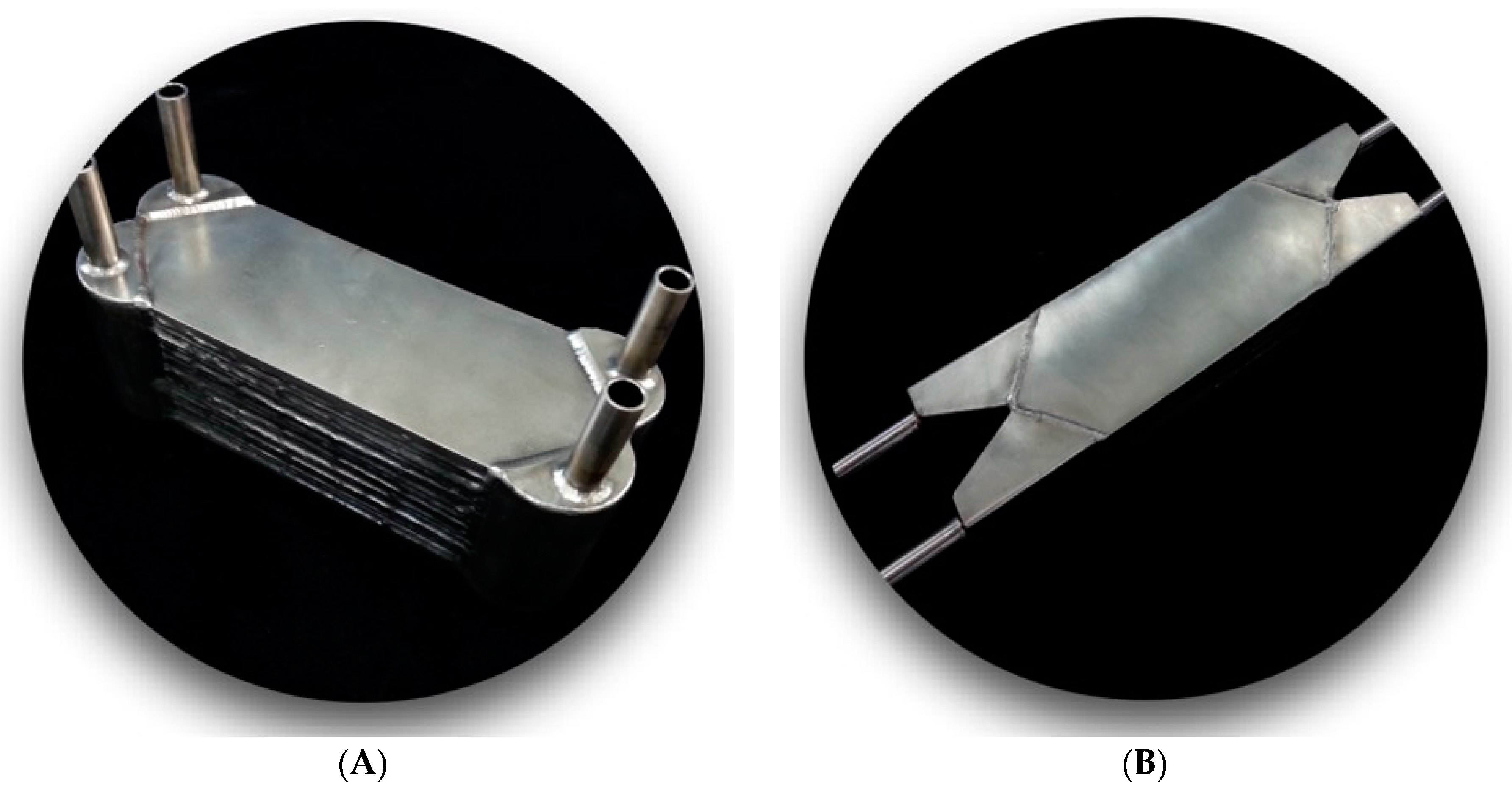
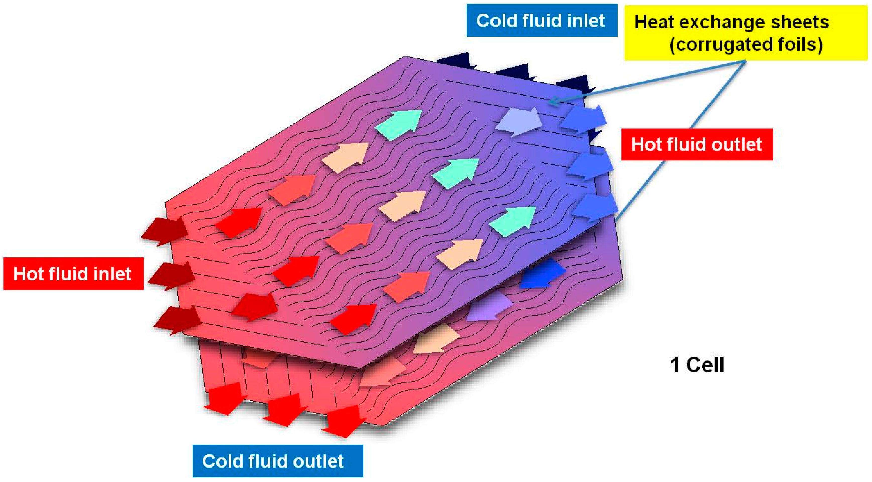
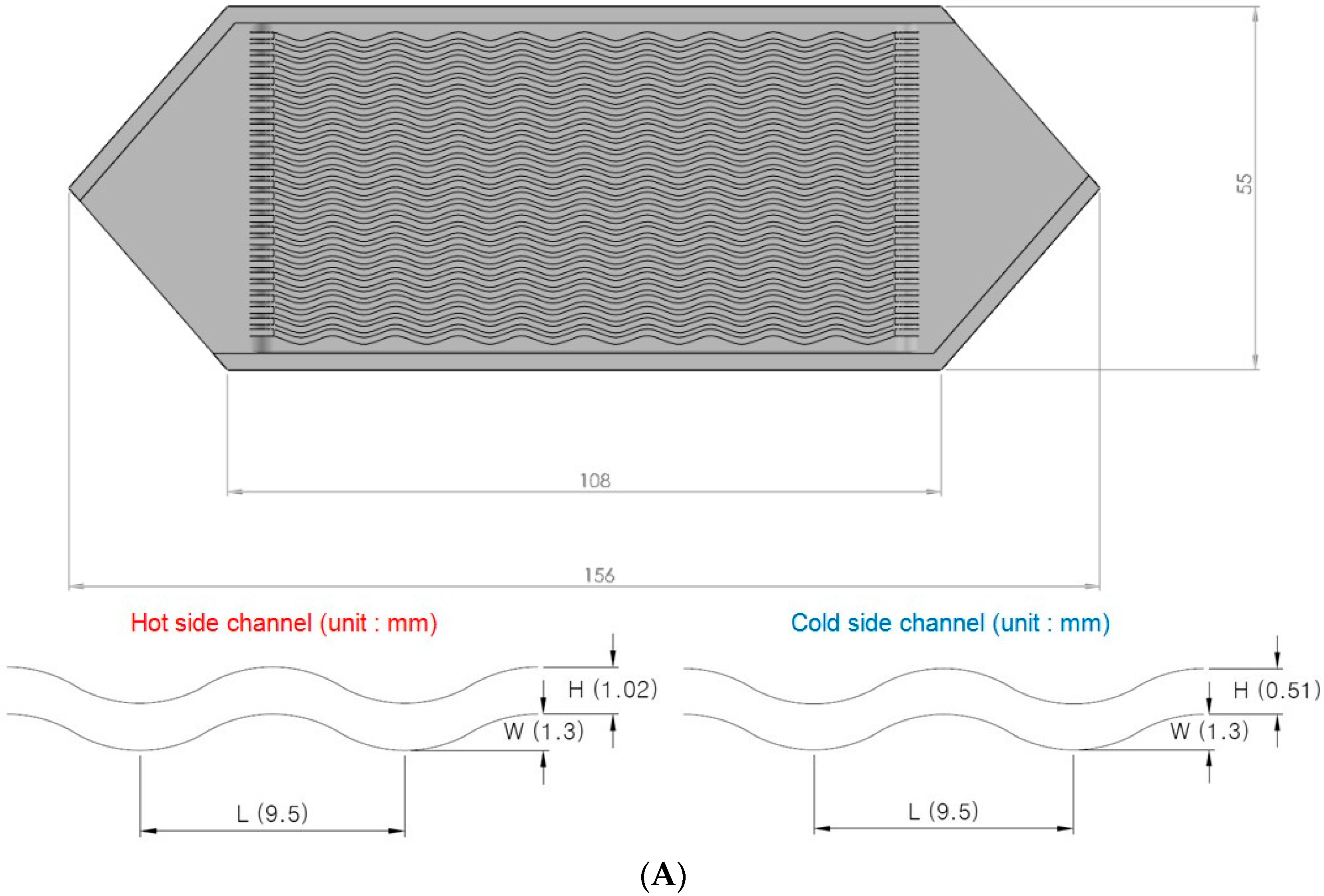
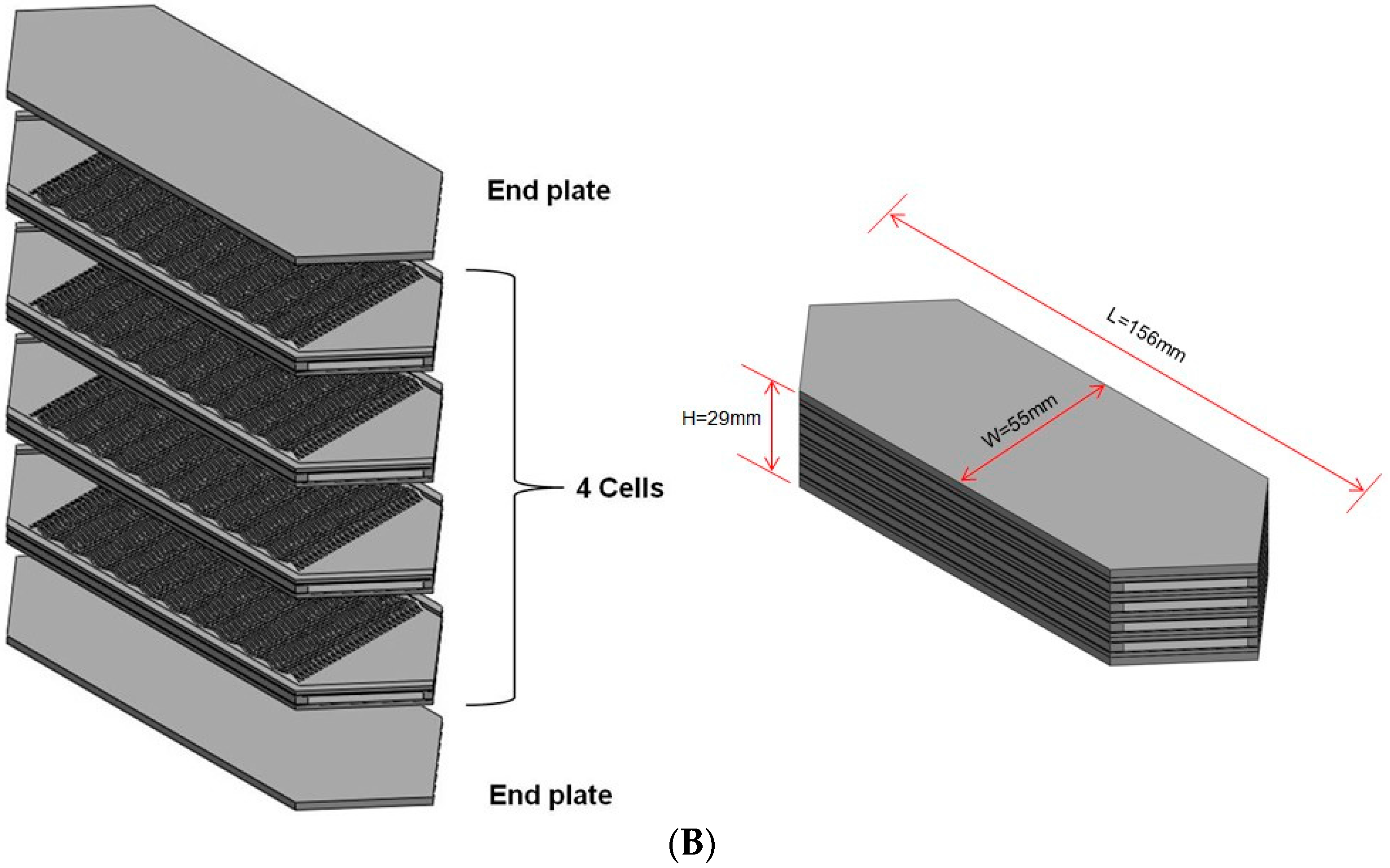
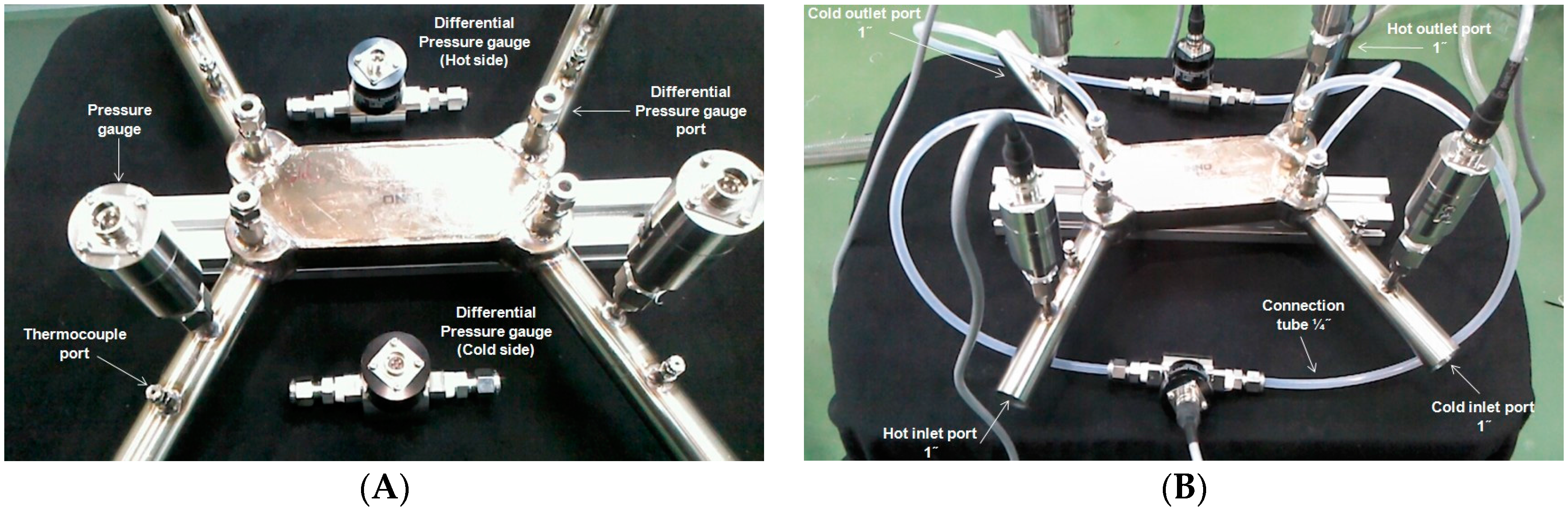
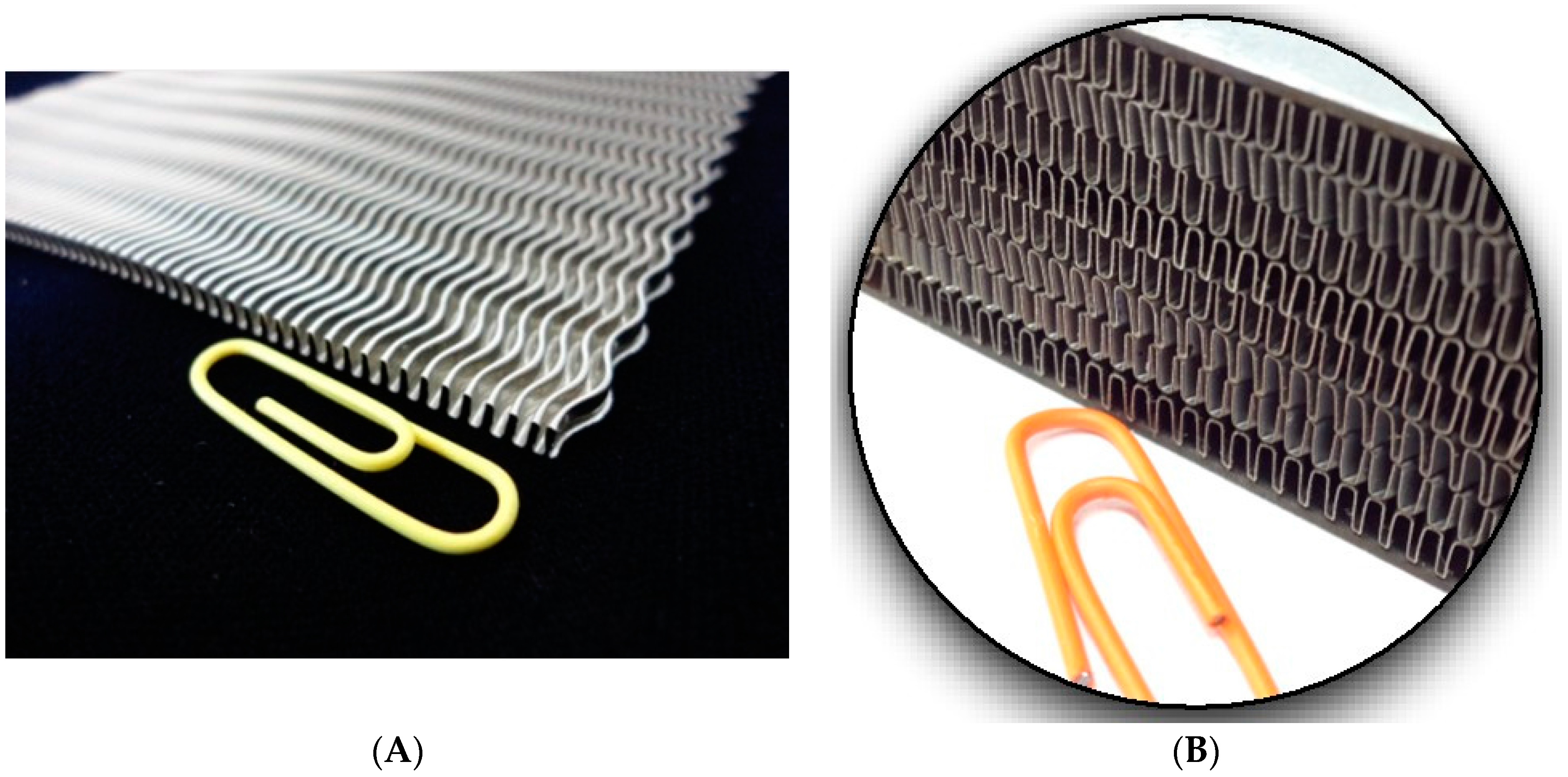
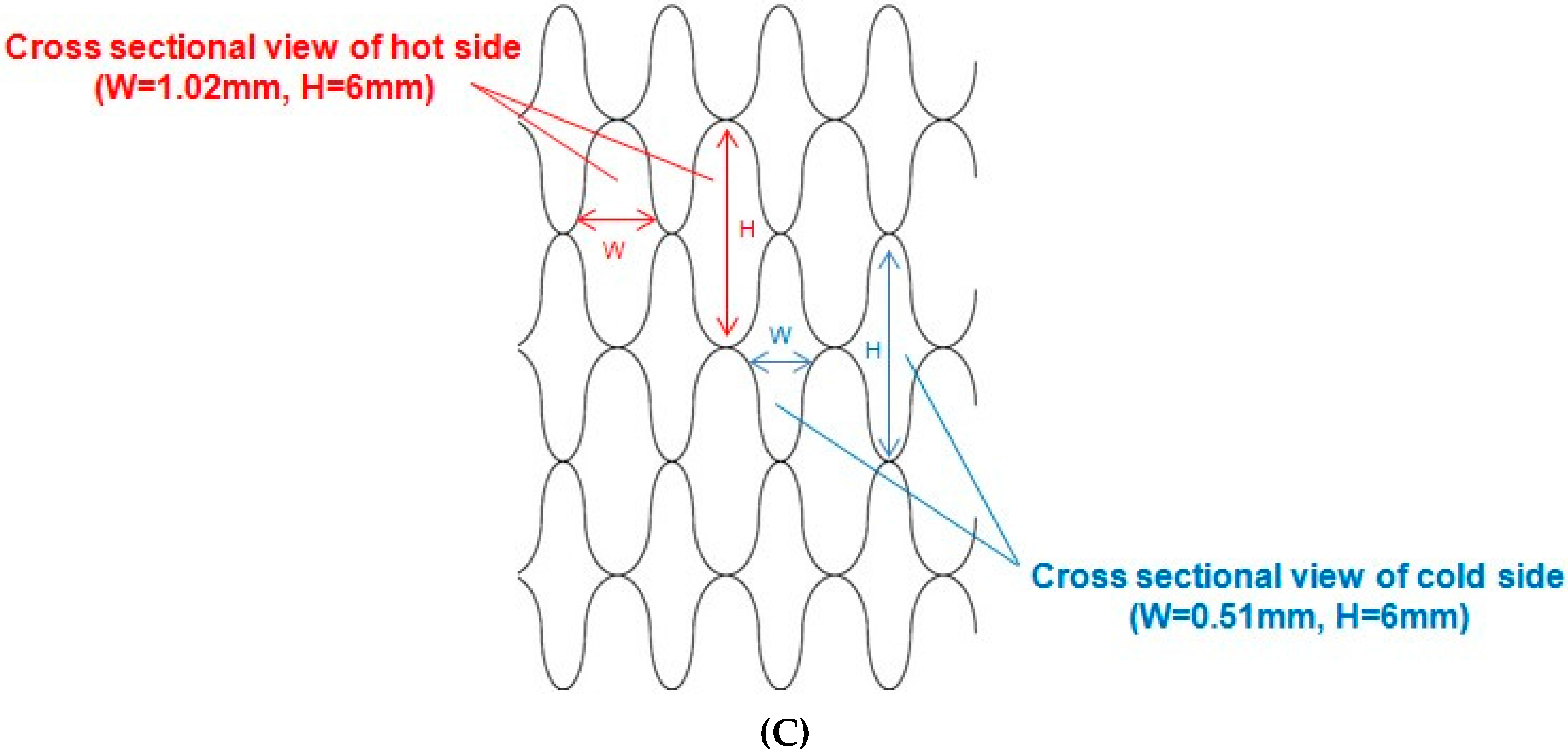
2.1. PSHE

Stainless Steel (STS) 316L was used as the material for the heat transfer plate with a total of eight heat transfer plates manufactured through compression processing. Two plates were joined to form a cell with a total of four cells created that were then stacked upon each other. To increase the internal pressure and structural strength, end plates were connected at both ends of the stacked heat transfer plates. After stacking the heat transfer plates, a bond was created through laser welding of the outer edge using a thin sheet of the same material. This resulted in a PSHE with 18 channels, four cells and eight plates, with this structure allowing for the necessary steady-state and constant inlet temperature condition required by this study. Two such PSHEs were manufactured—one to confirm manufacturing conditions and one for experimental use—with the detailed specification of these PSHEs presented in Figure 3A and Table 1. The manner of stacking the cells is shown in Figure 3B, and the PSHE used in the experiment is shown in Figure 4A; the PSHE before and after the installation of a pressure gauge and differential pressure gauge is shown in Figure 4A,B, respectively. To confirm the shape of the internal channels and the bonding condition of the heat transfer plates, one of the manufactured PSHEs was cut in half. The cross-section of one half of the cut PSHE and a photograph of the heat transfer plate are shown in Figure 5A,B. Figure 5B indicates that the bonding condition of the heat transfer plates was excellent. From this cut PSHE, the inlet area (A_c) and the effective heat transfer area (A_s) of the rounded channels were calculated. With regard to the fluid flow, a counterflow, which facilitates a high-temperature approach, was applied in this experiment, with the corrugated channels mixing the fluid flow from side to side in the direction of the working fluid’s movement.

Figure 3. Schematic geometry of corrugated surfaces (A); and stacked layers (B).

Figure 3. Schematic geometry of corrugated surfaces (A); and stacked layers (B).

Figure 4. The PSHE used in the experiment (A); and installed sensors (B).

Figure 4. The PSHE used in the experiment (A); and installed sensors (B).

Figure 5. The metal heat transfer plate (A); and cross-sectional view of the PSHE (B,C).

Figure 5. The metal heat transfer plate (A); and cross-sectional view of the PSHE (B,C).

Table 1. Specifications of the primary surface heat exchanger (PSHE).

Metal Plate Material	STS 316L
Dimensions of PSHE (W × L × H), mm	55 × 156 × 29
Dimensions of hot channel (W × L × H), mm	1.3 × 9.53 × 1.02
Dimensions of cold channel (W × L × H), mm	1.3 × 9.53 × 0.51
Channel height, mm	6
Number of plates	8
Number of cells	4
Number of channels	18
End plate thickness, mm	2.5

Table 1. Specifications of the primary surface heat exchanger (PSHE).

Metal Plate Material	STS 316L
Dimensions of PSHE (W × L × H), mm	55 × 156 × 29
Dimensions of hot channel (W × L × H), mm	1.3 × 9.53 × 1.02
Dimensions of cold channel (W × L × H), mm	1.3 × 9.53 × 0.51
Channel height, mm	6
Number of plates	8
Number of cells	4
Number of channels	18
End plate thickness, mm	2.5

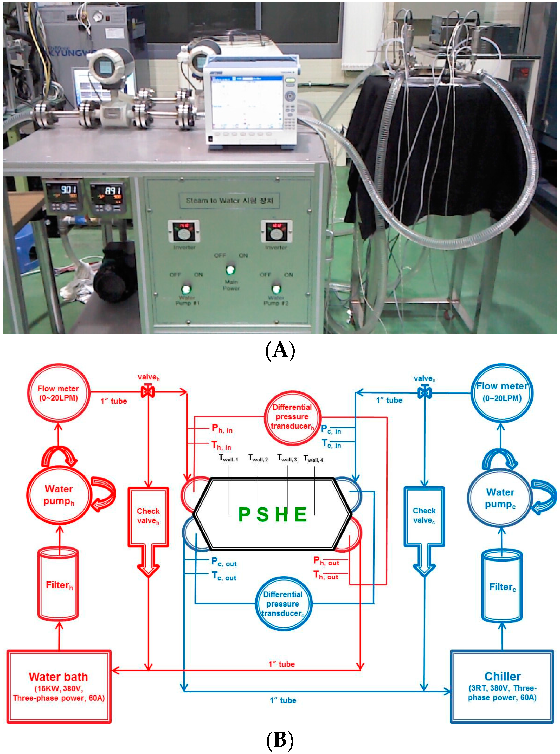
2.2. Experimental Equipment

The complete experimental setup is shown in Figure 6A. Figure 6B shows a schematic of the experimental system and the location of each measurement sensor. The experimental equipment consists of two sections—one circulating the hot fluid and the other circulating the cold fluid—and the PSHE, which exchanges heat between the hot and cold fluids. Thermostatic baths and water pumps were installed in each section in order to maintain a constant inlet temperature and flow rate for both the hot and cold fluids. To remove any foreign matter in the fluid, a filter was installed at the inlets of each water pump. A thermocouple, pressure gauge, differential pressure gauge and volumetric flow meter were also installed to measure the temperature, pressure and flow rate of the working fluid for the experiment. Before performing the experiment, the experiment system was operated for a minimum of 30 min to ensure that the appropriate inlet temperatures—40 °C for the hot side and 20 °C for the cold side—were reached. During this time, any bubbles generated from the flow of the working fluid were removed. When the measured inlet and outlet temperatures of the PSHE were different by no more than 0.5 °C, when the flow rates of the hot and cold sides were different by no more than 5%, when the heat balance, calculated based on the inlet and outlet temperatures of the hot and cold sides, of the hot and cold sides differed by less than 10% and after confirming the absence of leaks, a steady-state was considered to have been attained. When this steady-state condition was reached, data were collected at five-second intervals for 5 min. The following data were obtained: inlet and outlet temperatures at the hot and cold sides, pressure, differential pressure and end plate temperatures of the PSHE.

Figure 6. PSHE experimental apparatus. (A) Photograph of experimental apparatus; (B) schematic diagram of the experimental apparatus.

Figure 6. PSHE experimental apparatus. (A) Photograph of experimental apparatus; (B) schematic diagram of the experimental apparatus.

2.3. Experimental Conditions and Results Analysis

Water was used as the hot and cold fluid in this experiment, with the inlet temperature kept at 40 °C for the hot-side fluid and 20 °C for the cold-side fluid. The inflow rate was measured by increasing the hot-side flow rate while maintaining the same volumetric flow conditions and the cold-side flow rate. Based on the measured results, the volumetric flow rate ranged between 3 and 17 L/min, and the Reynolds number ranged between 156 and 921. The hydraulic diameter was calculated using a method proposed by Cowell [10], and the Reynolds number was calculated using Equations (1) and (2).

$$D_h=\frac{4A_c}{P}=\frac{4A_c{L}_f}{A_s}$$

(1)

$${\text{Re}}_h=\frac{G{D}_h}{\mu }=\frac{\dot{m}}{\mu }\frac{D_h}{A_c}$$

(2)

A_c is the free flow area; A_s is the total heat transfer area; and L_f is the length of a channel in the flow direction. At both ends, the total free flow area was 696 mm²; the total heat transfer area was 187,060 mm²; and L_f was 104.8 mm.

The heat transfer rates for the hot and cold sides were derived using Equations (3) and (4).

$$Q_h={\dot{m}}_h{C}_{p,h}\left(T_{h,i}-T_{h,o}\right)$$

(3)

$$Q_c={\dot{m}}_c{C}_{p,c}\left(T_{c,o}-T_{c,i}\right)$$

(4)

The overall heat transfer coefficient and heat transfer performance were obtained using Equations (7) and (8), and the log mean temperature difference (LMTD) was determined by Equation (5).

$$∆T_{LMTD}=\frac{\left(∆T_1-∆T_2\right)}{\text{ln}\left(∆T_1/∆T_2\right)}\{\begin{array}{c}∆T_1=T_{h,i}-T_{c,o}\\ ∆T_2=T_{h,o}-T_{c,i}\end{array}$$

(5)

$$Q_m=\frac{Q_h+Q_c}{2}$$

(6)

$$U=\frac{Q_m}{A_s∆T_{LMTD}}$$

(7)

$$UA=\frac{Q_m}{∆T_{LMTD}}$$

(8)

Generally, the overall heat transfer coefficient is represented by the sum of heat resistance, as shown in Equation (9).

$$\frac{1}{UA}=\frac{1}{{\left(hA\right)}_h}+\frac{t}{k{A}_m}+\frac{1}{{\left(hA\right)}_c}$$

(9)

Here, t, k and A_m denote the distance between the channels of the hot and cold sides, the heat conductivity of the heat transfer plate and the mean heat transfer area of hot and cold sides, respectively. The hot and cold side heat balance of the PSHE was calculated using Equation (10), and only the results that were within the 5% error range of heat quantity in the entire experiment were used.

$$Q_{loss}\left(\text{\%}\right)=\frac{\left|Q_h-Q_c\right|}{Q_h}$$

(10)

To evaluate the characteristics of the pressure drop of the PSHE, the f-factor was derived as shown in Equation (11).

$$f=\frac{A_c{\rho }_m}{A_s{\rho }_i}\left|\begin{array}{c}\frac{2{\rho }_i∆\text{P}}{{\left(\dot{m}/A_c\right)}^2}-\left(K_c+1-{\sigma }^2\right)\\ -2\left(\frac{{\rho }_i}{{\rho }_o}-1\right)+\left(1-{\sigma }^2-K_e\right)\frac{{\rho }_i}{{\rho }_o}\end{array}\right|$$

(11)

In Equation (11), σ is the contraction coefficient; the ratio of minimum free-flow area to the inlet and outlet port area. K_c and K_e are the contraction-loss coefficient and expansion-loss coefficient, respectively, and are calculated using a graph proposed by Kays and London [11] and Shen at al. [12]. The effects of gravity, generated by the difference in the amount of pressure drop and height owing to the fluid density at the inlet and outlet, were ignored.

2.4. Uncertainty

The experimental uncertainty of the PSHE was evaluated using ASME PTC 19.1 [13] and NIST Technical Note 1297 [14]. The uncertainty consists of the bias error and precision error, as shown in Equation (12). The uncertainty of a computational variable generated by error propagation was evaluated by Equation (13).

$$\text{Π}=2\sqrt{{\left(\frac{B}{2}\right)}^2+{\left(\frac{S}{\sqrt{N}}\right)}^2}$$

(12)

$${\text{Π}}_p=\sqrt{{\displaystyle \sum }_{i=1}^n{\left(\frac{\partial p}{\partial S_i}{u}_{si}\right)}^2}$$

(13)

Π is the total uncertainty; B is the bias error; S is the standard deviation; N is the number of measurements; and p is the computational variable. The details of the results of uncertainty analysis for this experiment are presented in Table 2.

Table 2. Parameters and estimated uncertainty.

Parameters	Uncertainty (%)
Temperature, T	0.31
Pressure drop, ΔP	0.94
Flow rate of hot side, ${\dot{m}}_h$	0.64
Flow rate of cold side, ${\dot{m}}_c$	0.78
Averaged heat transfer rate, Qm	1.19
Reynolds number of hot side	3.13
Reynolds number of cold side	3.29
Heat transfer coefficient of hot side	7.36
Heat transfer coefficient of cold side	7.31
Friction factor, f	5.2

Table 2. Parameters and estimated uncertainty.

Parameters	Uncertainty (%)
Temperature, T	0.31
Pressure drop, ΔP	0.94
Flow rate of hot side, ${\dot{m}}_h$	0.64
Flow rate of cold side, ${\dot{m}}_c$	0.78
Averaged heat transfer rate, Qm	1.19
Reynolds number of hot side	3.13
Reynolds number of cold side	3.29
Heat transfer coefficient of hot side	7.36
Heat transfer coefficient of cold side	7.31
Friction factor, f	5.2

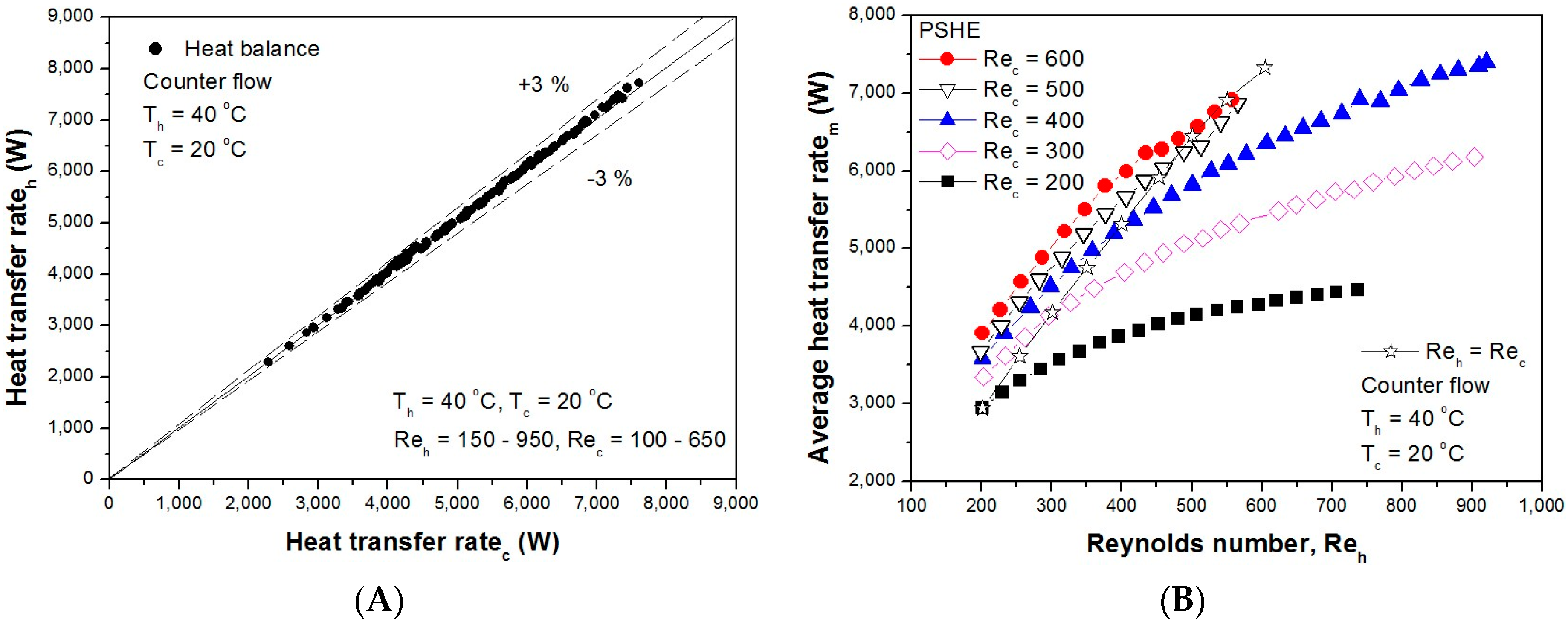
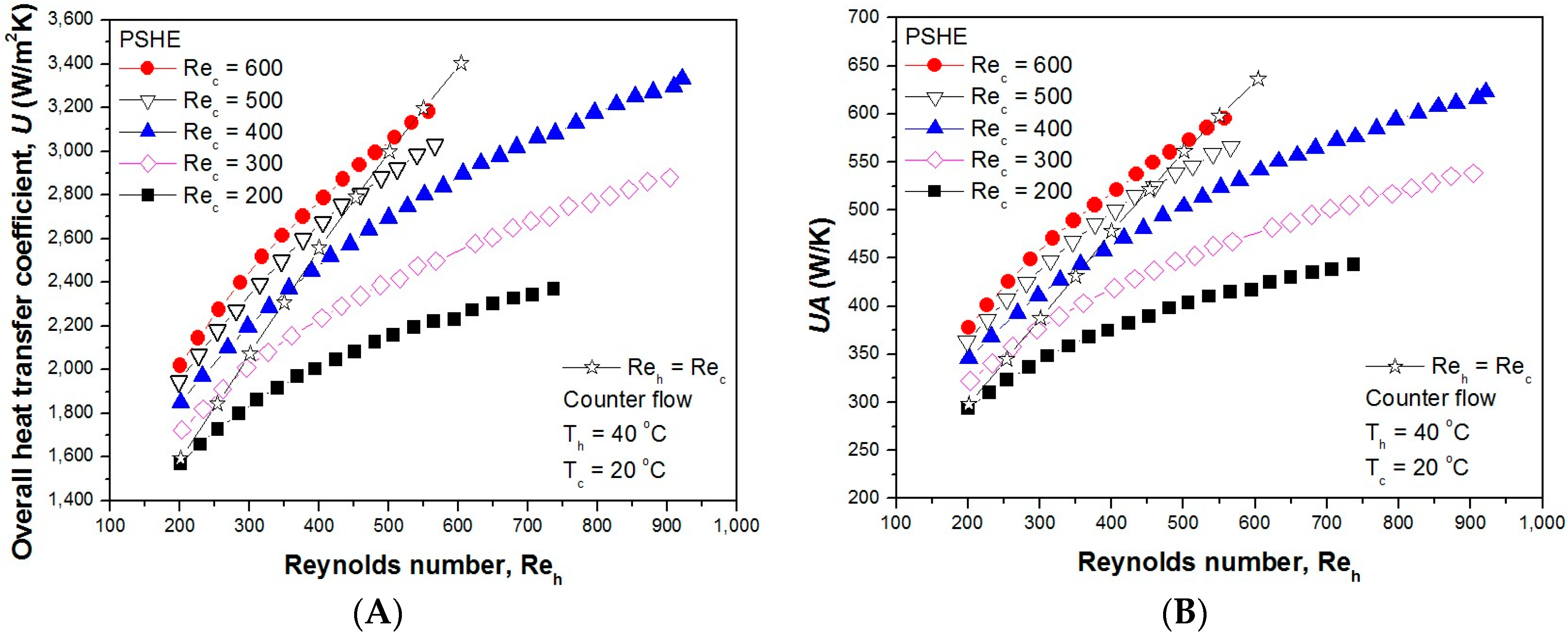
3. Experimental Results and Discussion

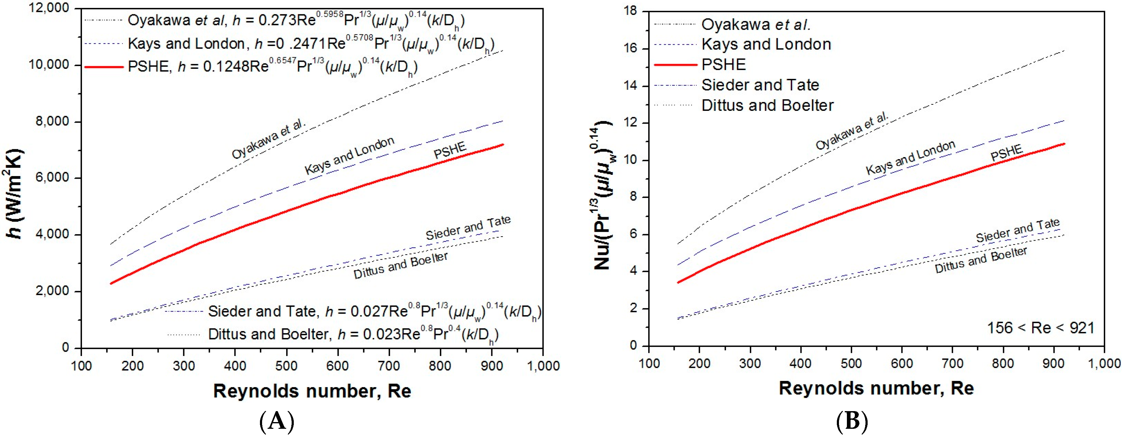
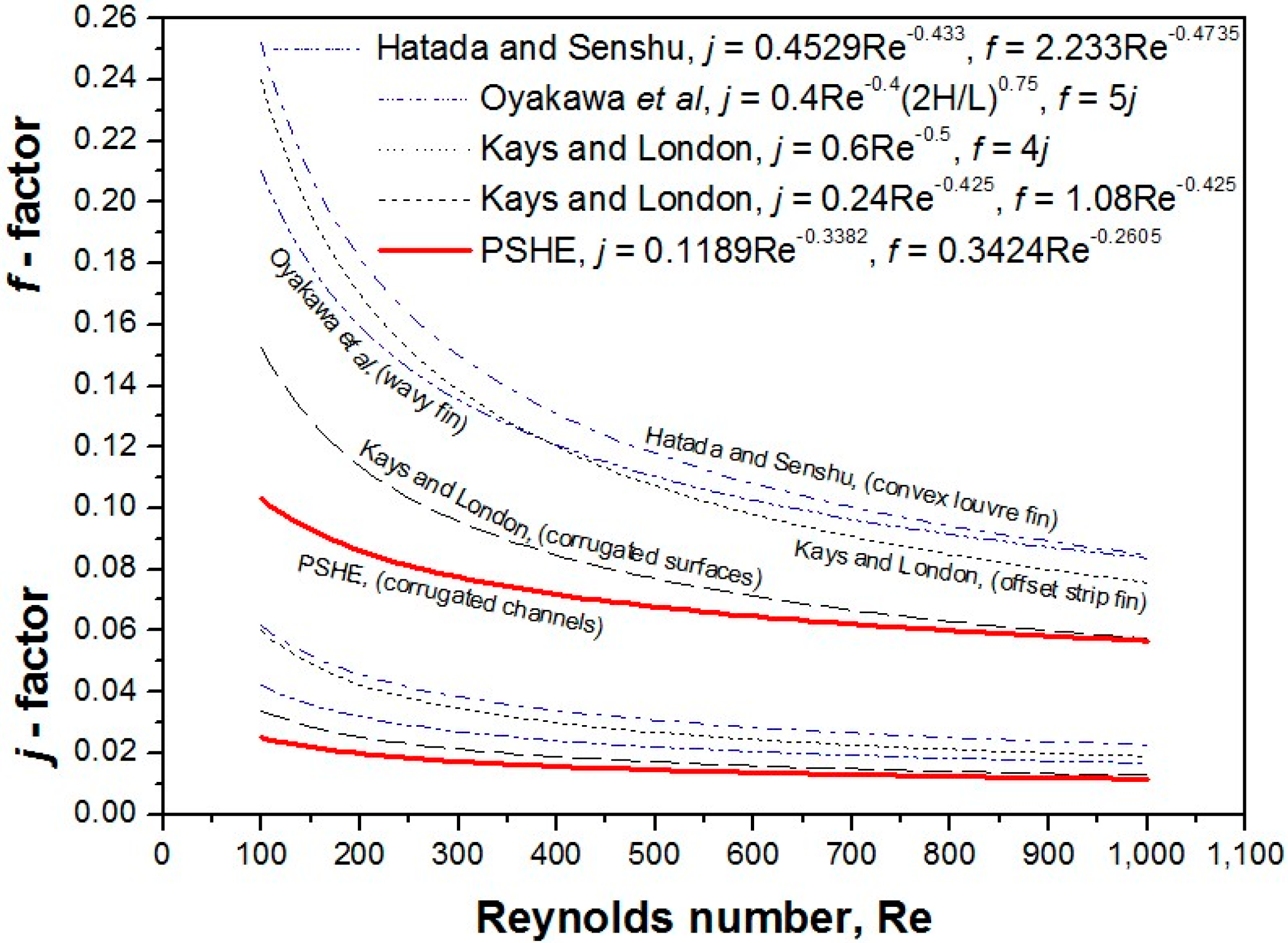
3.1. Heat Transfer Characteristics

The characteristics of heat transfer according to an increase in the Reynolds number were examined by fixing the inlet temperature of the hot side at 40 °C and the cold side at 20 °C. Figure 7A shows the thermal equilibrium of the hot and cold sections. The error of thermal equilibrium was within ±3%, and the reliability of the experimental apparatus and measurement equipment was determined to be excellent. Figure 7B shows a comparison of the mean heat transfer between two cases: one in which the Reynolds number at both sides increased constantly and one in which the Reynolds number of the hot side increased while the cold side had a fixed Reynolds number. This figure also shows that heat transfer increases as the Reynolds number of the fixed cold section increases or as the Reynolds number of both sides increases. This increase is due to the typical characteristics of thermal performance where the heat transfer rate increases as the flow rate increases. As the Reynolds number of the cold side increased by 100, the heat transfer rate increased by approximately 8% on average.

Figure 7. Heat balance and average heat transfer rate: (A) heat balance between hot and cold sides; (B) and cold side fixed Re conditions for the hot side increases.

Figure 7. Heat balance and average heat transfer rate: (A) heat balance between hot and cold sides; (B) and cold side fixed Re conditions for the hot side increases.

In Figure 8A, the overall heat transfer coefficient U is shown, and in Figure 8B, the heat transfer performance UA is shown. These figures show the results of the case when the Reynolds numbers of the hot and cold sections are the same and the case when the Reynolds number of the hot side increased while that of the cold side was fixed between 200 and 600. It was found that as the Reynolds numbers of the hot and cold sides increased, the overall heat transfer coefficient and heat transfer performance tended to increase. This is a result of the heat transfer rate increasing as the temperature difference between the inlet and outlet decreased. The overall heat transfer coefficient and heat transfer performance are represented as the ratio of the average heat transfer rate and log mean temperature difference, calculated from the difference between the inlet and outlet temperatures, in regard to an increasing Reynolds number. Namely, the log mean temperature difference has significant effects on the results. Moreover, it was found that the heat transfer performance was more rapid when the Reynolds numbers of both sides increased equally than when the Reynolds number of the cold side was fixed. This faster increase is because the flow rates of the hot and cold sides increased at the same time. Thus, this result indicates that an increase in the flow rates of both sides leads to high heat transfer performance.

Figure 8. Influence of Reynolds number. (A) Overall heat transfer coefficient (U) vs. Reynolds number; (B) heat transfer performance (UA) vs. Reynolds number.

Figure 8. Influence of Reynolds number. (A) Overall heat transfer coefficient (U) vs. Reynolds number; (B) heat transfer performance (UA) vs. Reynolds number.

In general, the heat transfer coefficient correlation in a single phase is commonly known to have the form of the Sieder–Tate Equation (14).

$$Nu=\left(\frac{h{D}_h}{k}\right)=C·{\text{Re}}^n·{\text{Pr}}^{1/3}{\left(\frac{\mu }{{\mu }_w}\right)}^{0.14}$$

(14)

where C is a constant; n is the Reynolds exponent; and µ_w is the average wall temperature of the end plates. To obtain the heat transfer coefficient of the hot and cold sides, a modified Wilson plot method [15,16,17] was used. The balance between the heat resistance and heat transfer coefficient of the hot and cold sections is shown in Equation (15) and is represented using the Reynolds number and Prandtl number with the power-law form.

$$\begin{array}{l}Y=\left[\frac{1}{UA}-\left(\frac{1}{k{A}_m}\right)\right]{\left[\frac{k}{D_h}{\text{Re}}^n{\text{Pr}}^{1/3}{\left(\frac{\mu }{{\mu }_w}\right)}^{0.14}A\right]}_h\hfill \\ X={\left[\frac{k}{D_h}{\text{Re}}^n{\text{Pr}}^{1/3}{\left(\frac{\mu }{{\mu }_w}\right)}^{0.14}A\right]}_h{\left[\frac{k}{D_h}{\text{Re}}^n{\text{Pr}}^{1/3}{\left(\frac{\mu }{{\mu }_w}\right)}^{0.14}A\right]}_c^{-1}\hfill \end{array}$$

(15)

where ${C^{\prime }}_{h^{\prime }}$, ${C^{\prime }}_{c^{\prime }}$ and Re were calculated by iterative multiple linear-regression analysis [18].

The result of the cold-side heat transfer experiment is shown in the modified Wilson plot in Figure 9. A correlation of the cold-side convective heat transfer coefficient within the Reynolds number range used is as shown in Equation (16).

$$\begin{array}{c}{h}_c=0.0848{\text{Re}}_c^{0.6547}{\text{Pr}}^{1/3}{\left(\mu /{\mu }_w\right)}_c^{0.14}{\left(k/D_h\right)}_c\\ 128<{\text{Re}}_c<622\end{array}$$

(16)

By using the proposed correlation of the cold-side heat transfer coefficient, the hot-side heat transfer coefficient could be obtained. The correlation of the hot-side convective heat transfer coefficient is shown in Equation (17).

$$\begin{array}{c}{h}_h=0.1248{\text{Re}}_h^{0.6547}{\text{Pr}}^{1/3}{\left(\mu /{\mu }_w\right)}_h^{0.14}{\left(k/D_h\right)}_h\\ 156<{\text{Re}}_h<921\end{array}$$

(17)

Figure 9. Typical modified Wilson plot results for the calibration of the cold-side heat transfer coefficient.

Figure 9. Typical modified Wilson plot results for the calibration of the cold-side heat transfer coefficient.

Figure 10A shows that the error range is within 10% when the hot-side convective heat transfer coefficient obtained through the experiment is compared to the value obtained using Equation (17).

Figure 10. Comparisons between suggested correlations and experimental data for hot-side heat transfer coefficients. (A) Heat transfer coefficient; (B) Nusselt number.

Figure 10. Comparisons between suggested correlations and experimental data for hot-side heat transfer coefficients. (A) Heat transfer coefficient; (B) Nusselt number.

Figure 10B shows the results of comparing the difference between the proposed correlation and the Nusselt number, a non-dimensional form, by using the calculated convective heat transfer coefficient. When these results are represented as a new correlation, it can be expressed as Equation (18).

$$Nu=0.1248{\text{Re}}^{0.6547}{\text{Pr}}^{1/3}{\left(\mu /{\mu }_w\right)}^{0.14}$$

(18)

The error range of the correlation of the heat transfer coefficient in this experiment is within ±10%, and the range of the Reynolds number is between 156 and 921.

Figure 11A,B shows the result of comparing the experimental results with the correlations of Oyakawa, Shinzato and Mabuchi and Kays and London [19], which, in terms of Reynolds number ranges and channel shape, are the most similar to the correlation proposed in this study. The Kays and London correlation shows a difference of 14.7% on average, and that of Oyakawa et al. shows a difference of 33% from the present results for the PSHE used in this study. The Sieder and Tate [20] correlation, which is well acknowledged as a fully-developed turbulent correlation, and the Dittus and Boelter [21] correlation had a difference of 46% on average in the smooth duct condition. This phenomenon is often observed in laminar flow, showing that the changes in the channel of the main flow and tube have a great effect on the convective heat transfer coefficient.

Figure 11. Comparison between suggested correlation and previous correlations. (A) Heat transfer coefficient; (B) Nusselt number.

Figure 11. Comparison between suggested correlation and previous correlations. (A) Heat transfer coefficient; (B) Nusselt number.

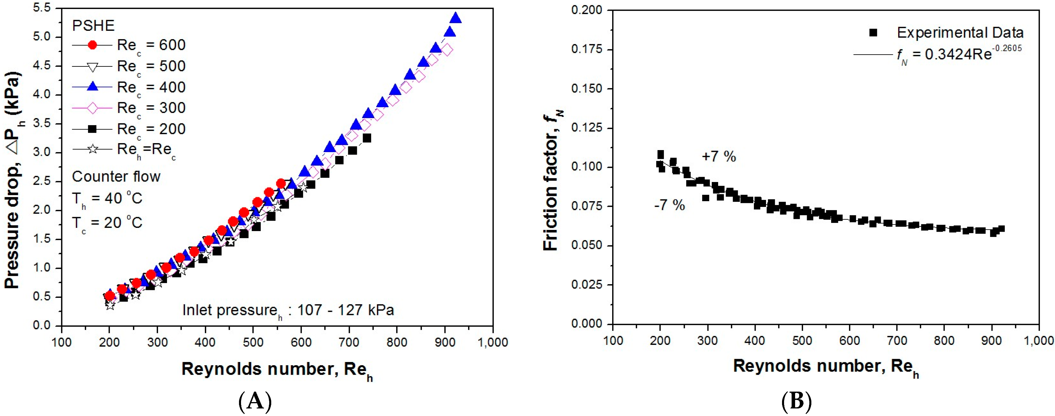
3.2. Pressure Drop Characteristics

Figure 12A shows the pressure drop results for the case in which the Reynolds numbers of both sides increased identically and for the case in which the hot-side flowrate was increased after fixing the cold-side Reynolds number between 200 and 600. In this figure, the pressure drop increased exponentially with an increasing Reynolds number. The Reynolds number was evaluated by the effects of viscosity according to the mass flow of the working fluid of varying temperatures. When the inlet temperature is low, the resistance of the working fluid increases in the channel, and as the Reynolds number increases, the pressure drop increases significantly. As the cold-side Reynolds number increased by 100, the hot-side pressure drop tended to increase by 1.2%–2.5%. This increase is because the hot-side working fluid’s viscosity increases in accordance with an increase in the Reynolds number of the cold-side.

Figure 12. Pressure drop and friction factor: (A) pressure drop vs. Reynolds number in all of the experiments; (B) friction factor vs. Reynolds number.

Figure 12. Pressure drop and friction factor: (A) pressure drop vs. Reynolds number in all of the experiments; (B) friction factor vs. Reynolds number.

Figure 12B shows a dimensionless friction factor according to the Reynolds number using Equation (11). In this figure, the subscript N refers to the number of stacked cells, and the correlation of the friction factor is represented as a function of the Reynolds number, as shown in Equation (19).

$$f_N=0.3424{\text{Re}}^{-0.2605},156<Re<921$$

(19)

The Reynolds number exponent was obtained using the least squares method. The correlation and experimental result show an error of ±7%, and the application range of Reynolds numbers is 156–921.

Figure 13 compares the friction factor previously proposed and the Colburn j-factor. The Colburn j-factor of the PSHE is expressed as shown in Equation (20).

$$j=0.1189{\text{Re}}^{-0.3382},156<Re<921$$

(20)

Figure 13. Comparison of friction factor (f-factor) and Colburn j-factor correlations vs. Reynolds number experimental data for the PSHE.

Figure 13. Comparison of friction factor (f-factor) and Colburn j-factor correlations vs. Reynolds number experimental data for the PSHE.

The proposed correlation was compared to the hydraulic diameter, the Reynolds number range and the existing correlations suggested for similar types of channels. When the proposed correlation was compared to the Kays and London corrugated surfaces correlation, which considered a Reynolds number range of 400–3000, there was a difference of approximately 12.3% from the f-factor and 15.3% from the j-factor on average. Oyakawa et al. utilized a Reynolds number range between 600 and 3000, with the proposed wavy fin-type correlation differing from theirs in terms of the f-factor and j-factor by approximately 38.8% and 34.3%, respectively. The results were similar to those from the offset strip fin-type correlation by Kays and London. The various studies by Hatada and Senshu for different angles of the convex Louvre fin gave higher results than those for the other fin types. Compared to the results of the correlations resulting from our experiment, the f-factor showed a difference of 43%, and the j-factor showed a difference of 53%.

Table 3 lists the dimensionless parameters and experimental data obtained for the hot side when the Reynolds numbers of both sides were identical.

Table 3. PSHE Experimental data values.

Parameters	Value
Mass flow rate, ${\dot{m}}_h$ (g/min)	3871	4884	5762	6693	7623	8608	9516	10,408	11,375
Mass flux, G (kg/m2∙s)	93	117	138	160	183	206	228	249	272
LMTD, (K)	9.9	10.5	10.8	11.0	11.1	11.3	11.5	11.6	11.5
Pressure drop, ΔP (kPa)	0.36	0.54	0.76	0.97	1.24	1.46	1.84	2.07	2.40
Heat transfer rate, Q (W)	2953	3631	4182	4763	5349	5956	6498	6994	7409
OHTC, U (W/m2∙K)	1595	1845	2073	2308	2557	2790	2998	3196	3404
UA (W/K)	298	345	388	432	478	522	561	598	637
Reynolds number, Reh = Rec	201	254	301	350	400	453	501	550	604
Prandtl number	4.86	4.83	4.82	4.81	4.80	4.78	4.77	4.76	4.73
HTC, h (W/m2∙K)	2692	3141	3503	3865	4212	4562	4871	5170	5488
Nusselt number	6.78	7.91	8.81	9.72	10.59	11.47	12.24	12.99	13.78
Friction factor, f	0.0861	0.0809	0.0774	0.0744	0.0719	0.0696	0.0678	0.0662	0.0646
Colburn j-factor, j	0.0198	0.0183	0.0173	0.0164	0.0157	0.0150	0.0145	0.0141	0.0136

Table 3. PSHE Experimental data values.

Parameters	Value
Mass flow rate, ${\dot{m}}_h$ (g/min)	3871	4884	5762	6693	7623	8608	9516	10,408	11,375
Mass flux, G (kg/m2∙s)	93	117	138	160	183	206	228	249	272
LMTD, (K)	9.9	10.5	10.8	11.0	11.1	11.3	11.5	11.6	11.5
Pressure drop, ΔP (kPa)	0.36	0.54	0.76	0.97	1.24	1.46	1.84	2.07	2.40
Heat transfer rate, Q (W)	2953	3631	4182	4763	5349	5956	6498	6994	7409
OHTC, U (W/m2∙K)	1595	1845	2073	2308	2557	2790	2998	3196	3404
UA (W/K)	298	345	388	432	478	522	561	598	637
Reynolds number, Reh = Rec	201	254	301	350	400	453	501	550	604
Prandtl number	4.86	4.83	4.82	4.81	4.80	4.78	4.77	4.76	4.73
HTC, h (W/m2∙K)	2692	3141	3503	3865	4212	4562	4871	5170	5488
Nusselt number	6.78	7.91	8.81	9.72	10.59	11.47	12.24	12.99	13.78
Friction factor, f	0.0861	0.0809	0.0774	0.0744	0.0719	0.0696	0.0678	0.0662	0.0646
Colburn j-factor, j	0.0198	0.0183	0.0173	0.0164	0.0157	0.0150	0.0145	0.0141	0.0136

4. Conclusions

In this study, an experiment was performed on the characteristics of heat transfer and pressure drop with changes in the Reynolds numbers of the hot and cold sides of a PSHE. The study proposes a heat transfer coefficient and dimensionless correlation based on the experiment results. It also compares the proposed correlation with existing correlations that are the most similar to the correlation of this study in terms of Reynolds number range and channel shape.

(1)

The average heat transfer rate increased as the flowrate increased because of an increase in the Reynolds number of the hot and cold sides.

(2)

Although the drop in pressure on the hot side increased with the cold-side Reynolds number, the amount of increase was insignificant. In addition, as the Reynolds numbers of the hot and cold sides increased simultaneously, the pressure drop increased.

(3)

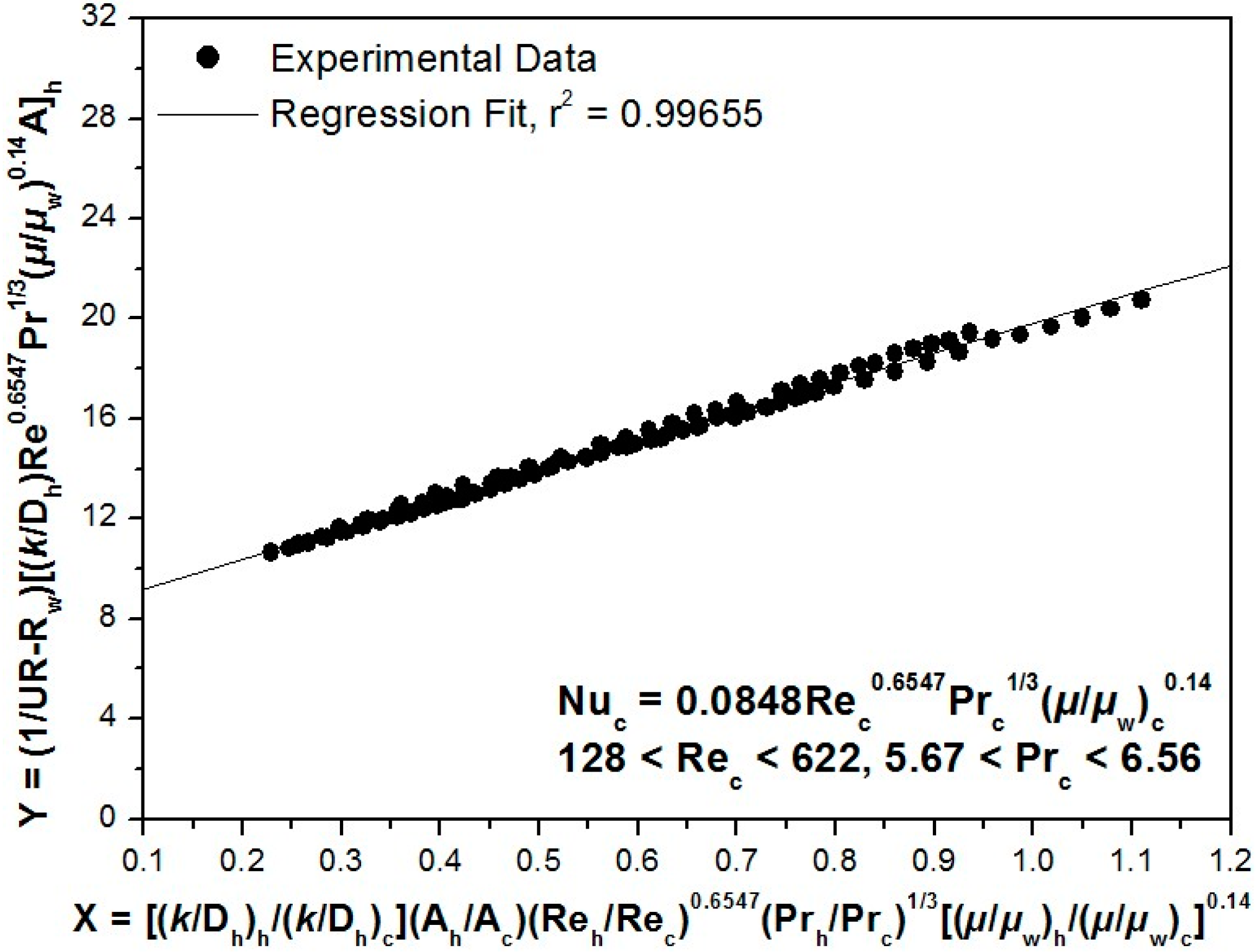
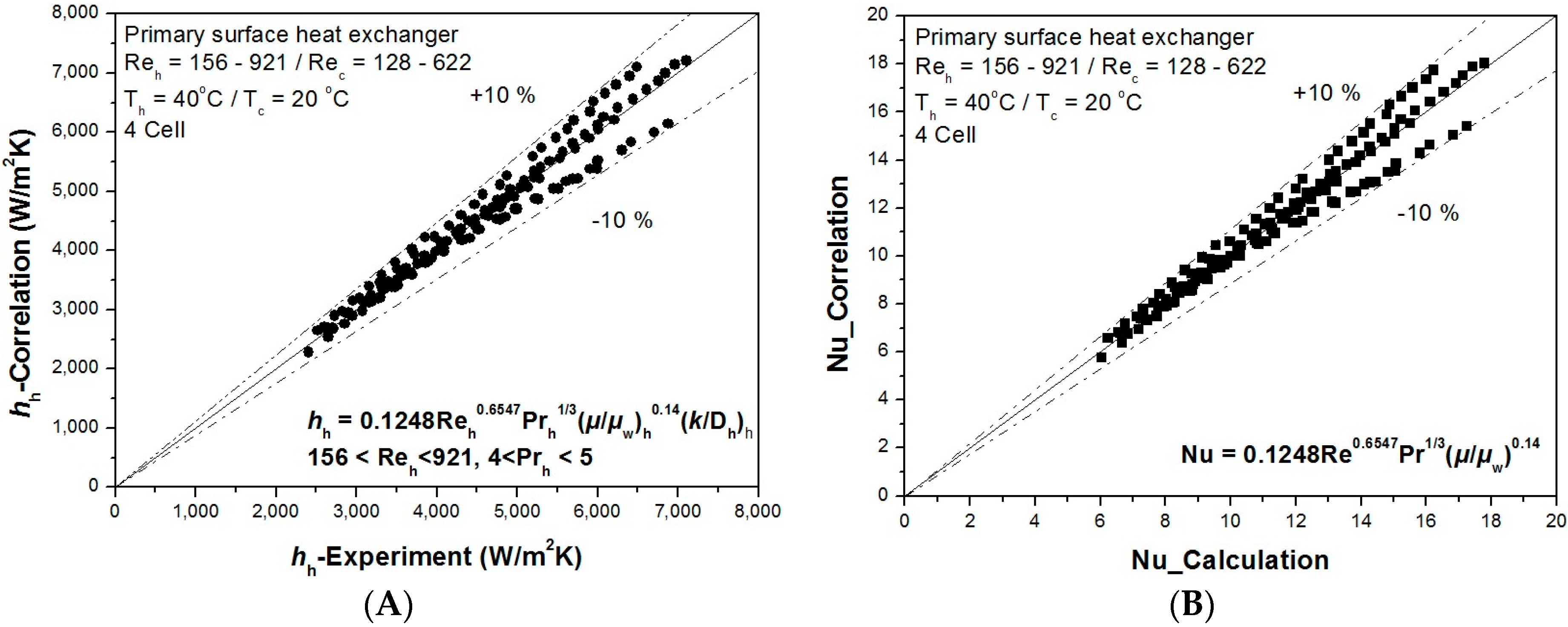
The correlation of the heat transfer coefficients of the hot and cold sides was proposed by applying the modified Wilson plot method to the heat transfer coefficient. For this correlation, the range of the Reynolds number was between 156 and 921.

(4)

The friction factor f was calculated by using the pressure drop results, and the appropriate friction factor correlation, for the PSHE examined in this study, was proposed.

References

1. Kim, M.S.; Ha, M.Y.; Min, J.K. Numerical study on the cross-corrugate primary surface heat exchanger having asymmetric cross-sectional profiles for advanced intercooled-cycle aero engines. Int. J. Heat Mass Trans. 2013, 66, 139–153. [Google Scholar] [CrossRef]
2. Ma, T.; Zeng, M.; Luo, T. Numerical study on thermo-hydraulic performance of an offset-bubble primary surface channels. Appl. Therm. Eng. 2013, 61, 44–52. [Google Scholar] [CrossRef]
3. Ma, T.; Zhang, J.; Borjigin, S. Numerical study on thermo small-scale longitudinal heat conduction in cross-wavy primary surface heat exchanger. Appl. Therm. Eng. 2015, 76, 272–282. [Google Scholar] [CrossRef]
4. Doo, J.H.; Ha, M.Y.; Min, J.K. An investigation of cross-corrugated heat exchanger primary surface for advanced intercooled-cycle aero engines. Int. J. Heat Mass Trans. 2012, 55, 5256–5267. [Google Scholar] [CrossRef]
5. Fsadni, A.M.; Ge, Y.T.; Lamers, A.G. Bubble nucleation on the surface of the primary heat exchanger in a domestic central heating system. Appl. Therm. Eng. 2012, 45–46, 24–32. [Google Scholar] [CrossRef]
6. Jeong, C.H.; Kim, H.R.; Ha, M.Y. Numerical investigation of thermal enhancement of plate fin type heat exchanger with creases and holes in construction machinery. Appl. Therm. Eng. 2014, 62, 529–544. [Google Scholar] [CrossRef]
7. Tang, L.H.; Zeng, M.; Wang, Q.W. Experimental and numerical investigation on air-side performance of fin-and-tube heat exchangers with various fin patterns. Exp. Therm. Fluid Sci. 2009, 33, 818–827. [Google Scholar] [CrossRef]
8. Pirompugd, W.; Wang, C.C.; Wongwises, S. Finite circular fin method for wavy fin-and-tube heat exchangers under fully and partially wet surface conditions. Int. J. Heat Mass Trans. 2008, 51, 4002–4017. [Google Scholar] [CrossRef]
9. Liu, Z.; Cheng, H. Multi-objective optimization design analysis of primary surface recuperator for microturbines. Appl. Therm. Eng. 2008, 28, 601–610. [Google Scholar]
10. Cowell, T.A. A general method for the comparison compact heat transfer surfaces. J. Heat Transf. 1990, 112, 288–294. [Google Scholar] [CrossRef]
11. Kays, W.M.; London, A.L. Compact Heat Exchangers, 2nd ed.; McGraw-Hill: New York, NY, USA, 1964. [Google Scholar]
12. Shen, S.; Xu, J.L.; Zhou, J.J.; Chen, Y. Flow and heat transfer in microchannels with rough wall surface. Energy Convers. Manag. 2006, 47, 1311–1325. [Google Scholar] [CrossRef]
13. ANSI/ASME PTC 19.1. In Measuring Uncertainty; The American Society of Mechanical Engineers: New York, NY, USA, 1998.
14. Taylor, B.N.; Kuyatt, C.E. Guidelines for Evaluating and Expressing the Uncertainty of NIST Measurement Results; NIST Technical Note 1297; U.S. Government Printing Office: Washington (DC), USA, 1994.
15. Shah, R.K. Assessment of modified Wilson plot techniques for obtaining heat exchanger design data. Heat Trans. 1990, 5, 51–56. [Google Scholar]
16. Wilson, E.E. A basis for rational design of heat transfer apparatus. Trans. ASME J. Heat Trans. 1915, 37, 47–82. [Google Scholar]
17. Hashmi, A.; Tahir, F. Empirical Nusselt number correlation for single phase flow through a plate heat exchanger. In Proceedings of the 9th WSEAS International Conference on Heat and Mass Transfer (HMT ’12), Cambridge, MA, USA, 25–27 January 2012; pp. 41–46.
18. Manglik, R.M.; Bergles, A.E. Heat Transfer Enhancement of Intube Flows in Process Heat Exchangers by Means of Twisted-Tape Inserts; Report No. HTL-18; Heat Transfer Laboratory, Rensselaer Polytechnic Institute: Troy, NY, USA, 1991. [Google Scholar]
19. Hesselgreaves, J.E. Compact Heat Exchangers; Pergamon: Edinburgh, UK, 2001. [Google Scholar]
20. Sieder, E.N.; Tate, G.E. Heat transfer and pressure drop of liquid in tubes. Ind. Eng. Chem. 1936, 28, 1429–1435. [Google Scholar] [CrossRef]
21. Dittus, F.W.; Boelter, L.M.K. Heat transfer in automobile radiators of the tubular type. Int. Commun. Heat Mass Transf. 1985, 12, 3–22. [Google Scholar] [CrossRef]