Measure of Uncertainty in Process Models Using Stochastic Petri Nets and Shannon Entropy

Abstract

When modelling and analysing business processes, the main emphasis is usually put on model validity and accuracy, i.e., the model meets the formal specification and also models the relevant system. In recent years, a series of metrics has begun to develop, which allows the quantification of the specific properties of process models. These characteristics are, for instance, complexity, comprehensibility, cohesion, and uncertainty. This work is focused on defining a method that allows us to measure the uncertainty of a process model, which was modelled by using stochastic Petri nets (SPN). The principle of this method consists of mapping of all reachable marking of SPN into the continuous-time Markov chain and then calculating its stationary probabilities. The uncertainty is then measured as the entropy of the Markov chain (it is possible to calculate the uncertainty of the specific subset of places as well as of whole net). Alternatively, the uncertainty index is quantified as a percentage of the calculated entropy against maximum entropy (the resulting value is normalized to the interval <0,1>). The calculated entropy can also be used as a measure of the model complexity.

1. Introduction

In recent years, a research area that focuses on the analysis of process models began to develop and since then a number of various specific metrics has been defined that allow the quantification of different characteristics of process models. These characteristics include, for instance, complexity [1,2], uncertainty [3], cohesion [4] or fairness [5]. These metrics are then used to analyse user-friendliness, usability, comprehensibility, predictability and other indicators [6]. In the following, a procedure (process) is designed for the analysis and evaluation of uncertainty of any process model represented using stochastic Petri nets (SPN). The use of stochastic Petri nets carries the advantage of options to define the probability of each branch by default (e.g., XOR) in the form of firing-rates of the individual transitions. By considering the probability of branching, it is possible to quantify the dynamic uncertainty, which takes into account both the model structure and the branching probabilities. Likewise, it is possible to quantify only the static uncertainty, which does not specify the probability of branching (all paths have the same probability) [7]. Quantification of uncertainty of process models represents the expected behaviour of the modelled process, i.e., its degree of predictability. Reducing uncertainty in the process model (e.g., by adjustment of structure or branching probabilities) can lead to better predictability of the real state of the modelled process and better managerial effectiveness associated with its management.

Stochastic Petri nets are an appropriate tool for modelling a series of problems, characterized by concurrency, asynchronous processing and non-determinism. One of the areas where it is possible to take advantage of Petri nets (mainly because of an exact mathematical foundation) is the process modelling. In this article, therefore, the issue of uncertainty in stochastic Petri nets will be presented on process models. However, conclusions and the method itself are universal and can be applied and interpreted on any issue that can be modelled with stochastic Petri nets.

The aim of this work is to define a method that allows us to quantify the uncertainty of any process model represented with stochastic Petri nets. The method quantifies the uncertainty using the concept of stochastic processes (continuous-time Markov chains) and information theory (Shannon's entropy [8]).

2. Petri Nets

Petri nets have been defined in 1962 by Carl Adam Petri [9] and since then, their development has begun to take different directions (mainly two directions). The first direction leads to new model features that extend the verification capabilities of Petri nets. These features are primarily behavioural properties of Petri net such as boundedness, liveness, reachability, fairness and many more. Almost all of these behavioural properties require specific assumptions that restrict the definition of Petri net, e.g., for verification of most of these properties it is required the assumption of pure net (network without self-cycles) or some algorithms will work only with ordinary nets (multiplicity of all arcs is equal one). The second direction leads to expansion of the Petri net definition by adding new additions that simplify and refine modelling (sometimes leads to a lower degree of formality). The most common examples of this second direction are stochastic and timed Petri nets that allow refining of the individual state changes by taking into account the time consumption (stochastically or deterministically). Different example are coloured Petri nets (CPN), which expands the basic Petri net with additional modelling language, thus expanding (partly simplifying) the modelling capabilities of Petri nets. The biggest drawback of most Petri net extensions in this direction is limited analytical options, i.e., most of the assumptions need to be verified by using the simulation.

The following is the definition of stochastic Petri net [10,11]. Solid introduction to issue of stochastic Petri nets can be found in [12].

Definition 1: Stochastic Petri net is a 5-tuple, $SPN = \left(P, T, F, \mathsf{\Lambda }, M_0\right)$ where:

• $P = \left\{ p_1,p_2,\dots , p_m\right\}$ – a finite set of places,
• $T = \left\{t_1,t_2,\dots , t_n\right\}$– a finite set of transitions,
• $P {{\displaystyle \cap }}^{\text{}} T = \varnothing$ – places and transitions are mutually disjoint sets,
• $F \subseteq \left(P \times T\right) {{\displaystyle \cup }}^{\text{}} \left(T \times P\right)$ – a set of edges, defined as a subset of the set of all possible connections,
• $\mathsf{\Lambda }:T \to R^{+}$ – firing rates of exponentially distributed timed transitions,
• $M_0:P \to N_0$ – an initial marking.

Definition 2: Marking of stochastic Petri net

Let $SPN = \left(P, T, F, \mathsf{\Lambda }, M_0\right)$be a stochastic Petri net. $M:P \to N_0$, is called marking of $SPN$.

Marking of Petri net represents the network state after execution of a specific number of steps, i.e., after firing of a specific number of enabled transitions.

Definition 3: Pre-set, Post-set

Let $SPN = \left(P, T, F, \mathsf{\Lambda }, M_0\right)$be a stochastic Petri net. Pre-sets and post-sets are defined as:

• ${}^{•}p=\left\{t\right|\left(t,p\right)\in F\}$ – the pre-set of $p$,
• ${}^{•}t=\left\{p\right|\left(p,t\right)\in F\}$ – the pre-set of $t$,
• $p^{•}=\left\{t\right|\left(p,t\right)\in F\}$ – the post-set of $p$,
• $t^{•}=\left\{p\right|\left(t,p\right)\in F\}$ – the post-set of $t$.

Definition 4: Enabled transition

Let $SPN = \left(P, T, F, \mathsf{\Lambda }, M_0\right)$be a stochastic Petri net. A transition $t \in T$ is enabled within marking $M$, if:

$$\forall p\in {}^{•}t:M\left(p\right)\ge 1$$

Definition 5: Next marking

Let $SPN = \left(P, T, F, \mathsf{\Lambda }, M_0\right)$be a stochastic Petri net and $M$ is its marking. If a transition $t\in T$ is enabled at marking $M$, then by its execution is obtained next marking $M´$, which is defined as follows:

$$\forall p\in P:M´\left(p\right)=\{\begin{array}{ll}M\left(p\right)-1,\hfill & if p\in {}^{•}t\backslash t^{•}\hfill \\ M\left(p\right)+1,\hfill & if p\in t^{•}\backslash {}^{•}t\hfill \\ M\left(p\right)\hfill & otherwise\hfill \end{array}$$

The situation that the transition $t$ changes the marking $M$ to $M´$ is usually expressed as $M[t\rangle M´.$

Definition 6: Reachability, sequence of transitions

Let $SPN = \left(P, T, F, \mathsf{\Lambda }, M_0\right)$be a stochastic Petri net. A sequence of transitions $\sigma$ is the succession of enabled transitions that goes from marking $M$ to different marking $M´$. The situation is referred to as $M[\sigma \rangle M´$. A marking is called reachable if there is a sequence of transitions to it from the initial marking.

Definition 7: The set of all reachable marking

Let $SPN = \left(P, T, F, \mathsf{\Lambda }, M_0\right)$be a stochastic Petri net. The set of all reachable markings from initial marking M₀ in $SPN$ is denoted by $R\left(M_0\right)$

$$R\left(M_0\right)=\left[\begin{array}{cccc}{M}_0\left(p_1\right)& M_1\left(p_1\right)& \cdots & M_{\left|R\left(M_0\right)\right|}\left(p_1\right)\\ M_0\left(p_2\right)& M_1\left(p_2\right)& \cdots & M_{\left|R\left(M_0\right)\right|}\left(p_2\right)\\ ⋮& ⋮& \ddots & ⋮\\ M_0\left(p_m\right)& M_1\left(p_m\right)& \cdots & M_{\left|R\left(M_0\right)\right|}\left(p_m\right)\end{array}\right].$$

Definition 8: Boundedness

Let $SPN=\left(P,T,F,\text{Λ},M_0\right)$ be a stochastic Petri net. Place $p\in P$ is called $k-bounded$ if:

$$\exists k\in N_1:\forall M\in R\left(M_0\right):M\left(p\right)\le k$$

Place $p\in P$ is called bounded, if it is $k-bounded$ for some $k\in N_1$. If every place in $SPN$ is bounded, then this net is called bounded Petri net.

Definition 9: Live marking, live net

Let $SPN = \left(P, T, F, \mathsf{\Lambda }, M_0\right)$be a stochastic Petri net. Marking $M\in R\left(M_0\right)$ is live, if $\forall t\in T$ there exist some marking $M_1\in R\left(M\right)$ such that transition $t$ is $M_1$-enabled. An SPN is live iff all reachable markings are live.

3. Steady-State Probability of Markings and Markov Chains

According to [10] it is possible to represent the set of all reachable markings in terms of Markov chains. Firstly, for the need of defining the stationary probabilities of all marking it is necessary to define the transition rate matrix.

Definition 10: Transition rate matrix

Let $SPN = \left(P, T, F, \mathsf{\Lambda }, M_0\right)$be a stochastic Petri net and $R\left(M_0\right)$ its reachability set. Transition rate matrix $\mathit{Q}$ of $SPN$ is defined as:

$$Q:\left(R\left(M_0\right)\times R\left(M_0\right)\right)\to R$$

The values are made according to the following rule:

$$Q_{i,j}=\{\begin{array}{cc}{\displaystyle \sum }_{t_k\in \left\{h:h\in T\wedge M_i\ge 1\wedge M_i[h{M}_j\right\}}{\lambda }_k,& if i\ne j\\ -{\displaystyle \sum }_{M_k\in \left\{h:h\in R\left(M_0\right)\wedge i\ne k\right\}}{Q}_{i,k},& if i=j\end{array}$$

Definition 11: Steady-State probability

Let $SPN = \left(P, T, F, \mathsf{\Lambda }, M_0\right)$be a stochastic Petri net and $\mathit{Q}$ its transition rate matrix. Steady-State distribution vector $\mathit{\eta }$ is defined as normalized left null space of transition matrix$\mathit{Q}$:

$$\mathit{\eta }Q=0$$

$$\eta 1^T=1$$

Vector $\mathit{\eta }$ represents the steady-state probability of each $SPN$ marking:

$$\eta =\left[\begin{array}{c}Pr\left(M_0\right)\\ Pr\left(M_1\right)\\ ⋮\\ Pr\left(M_{\left|R\left(M_0\right)\right|}\right)\end{array}\right]$$

Long term probability of marking $M\in R\left(M_0\right)$ is defined as a corresponding element of vector $\mathit{\eta }:$

$${\eta }_i=Pr\left(M_i\right)$$

The probability of marking can be viewed as a joined probability of individual places in a specific marking.

$$Pr\left(M\right)=Pr\left(M\left(p_1\right)=x_1,M\left(p_2\right)=x_2,\dots ,M\left(p_m\right)=x_m\right)$$

In the calculation of steady-state probabilities it is appropriate to ensure the liveness of Petri net model, since each dead marking corresponds to an absorbing state in the Markov chain. Every absorbing state can always occur, i.e., its stationary probability is equal to 1 and thus all live markings have stationary probabilities equal to 0. This would lead to a fully deterministic model without any uncertainty. It is also necessary to ensure the boundedness of the Petri net in order to ensure that the set of reachable markings is finite (unbounded Petri net = infinite number of all reachable markings).

4. Entropy

Entropy can measure the amount of disorder (uncertainty) that is associated with a random variable.

Definition 12: The entropy of the random variable X is defined (with the assumption $0·{\log }_2\left(0\right)\equiv 0$) as:

$$H\left(X\right)=-{\displaystyle \sum }_{x}Pr\left(X=x\right){\log }_{2}Pr\left(X=x\right)$$

Definition 13: Entropy of stochastic Petri net

Let $SPN = \left(P, T, F, \mathsf{\Lambda }, M_0\right)$be a stochastic Petri net and $\mathit{\eta }$is the vector of its stationary probabilities ${\eta }_i=\mathrm{Pr}\left(M_i\right), M_i\in R\left(M_0\right)$. The entropy of the $SPN$ is defined as:

$$H\left(SPN\right)=-{\displaystyle \sum }_{i=1}^{\left|R\left(M_0\right)\right|}{\eta }_i{\log }_2{\eta }_i$$

Definition 14: Uncertainty Index of stochastic Petri net

Let $SPN = \left(P, T, F, \mathsf{\Lambda }, M_0\right)$ be a stochastic Petri net and $H\left(SPN\right)$ its entropy. Uncertainty index of $SPN$ is defined as:

$$Uncertainty Index\left(SPN\right)=\frac{H\left(SPN\right)}{{\log }_2\left|R\left(M_0\right)\right|}$$

The normalization with maximum entropy makes the uncertainty index a dimensionless quantity which is suitable for the comparison of models with a different number of reachable markings. The uncertainty index value is from the interval <0,1>, where 0 interprets the fully deterministic model and 1 the absolute chaotic model. When the value of uncertainty index is closer to 1, the less is predictable the behaviour of the model. Furthermore, it is possible to use entropy as a measure of complexity, which reflects the size of the model (the number of reachable markings).

5. Example

In this work, we chose to present the measure of uncertainty through a simple example, mainly because of the applicability of this method in the broad area of subjects that use Petri nets as a tool for modelling and verification. The use of a more complex example would be beyond the scope of the article and moreover, the essence of the method would be hidden by the complexity of the example.

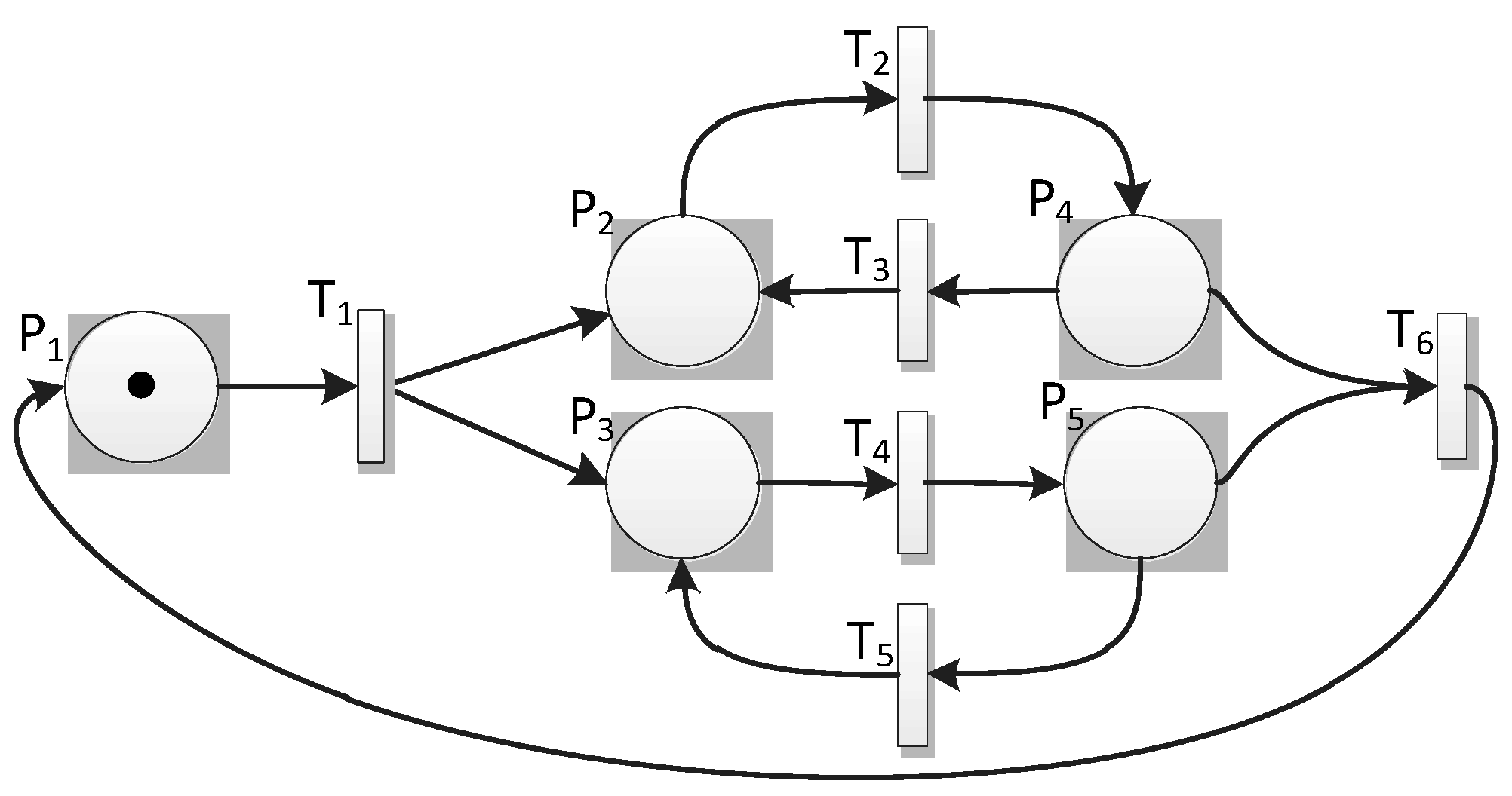
In the following is presented an example of stochastic Petri net which consists of 6 transitions and 5 places, see Figure 1. The example contains the essential characteristic features that are included in the process model. These elements are, for instance, the sequence (e.g., transition T₄), AND-split (transition T1), AND-join (transition T₆), XOR (transitions T₆ and T₅ or T₆ and T₃) and cycle (transition T₆ to place P₁). More information about the mapping of these and other elements into Petri nets can be found in [3].

Figure 1. Example of a stochastic Petri net (SPN).

Figure 1. Example of a stochastic Petri net (SPN).

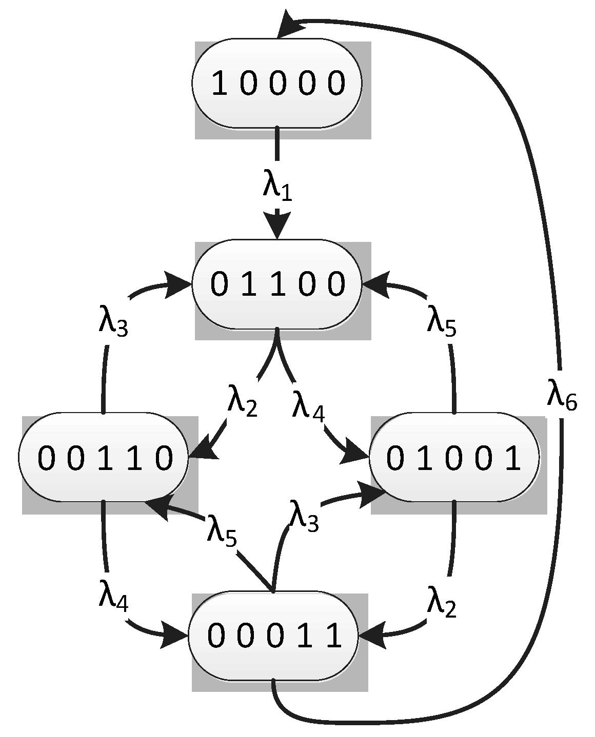
All reachable markings $R\left(M_0\right)$ of this example Petri net are as follows:

$$\begin{array}{cccccc}& M_0& M_1& M_2& M_3& M_4\\ p_1& 1& 0& 0& 0& 0\\ p_2& 0& 1& 0& 1& 0\\ p_3& 0& 1& 1& 0& 0\\ p_4& 0& 0& 1& 0& 1\\ p_5& 0& 0& 0& 1& 1\end{array}$$

Taking into account the specific values of transition firing rates, for instance, $\mathsf{\Lambda }=\left({\lambda }_1,{\lambda }_2,{\lambda }_3,{\lambda }_4,{\lambda }_5,{\lambda }_6\right)$, the given net is shown in Figure 2 as a Markov chain.

Figure 2. Corresponding Markov chain.

Figure 2. Corresponding Markov chain.

It is then possible to calculate the steady-state probability vector. The solution of this chain, for $\mathsf{\Lambda }=\left(5,2,3,3,2,1\right)$ is the steady-state probability vector:

$$\mathit{\eta }=\left[\begin{array}{c}0.0385\\ 0.2692\\ 0.1538\\ 0.3462\\ 0.1923\end{array}\right]$$

The entropy of the example network can then be expressed by:

$$H\left(SPN\right)=-(0.0385{\log }_{2}0.0385+0.2692{\log }_{2}0.2692+0.1538{\log }_{2}0.1538+0.3462{\log }_{2}0.3462+0.1923{\log }_{2}0.1923)=2.093$$

Reference limit (maximum entropy) is in this case${\log }_{2}5=2.3219$. The value of entropy itself can be useful when comparing the complexity of the model when changing its structure, i.e., as an alternative to the known measures of complexity (e.g., [3] or [13]). However, if we want to express the position of the complexity to the maximum complexity, which the model can have with the given structure, the initial marking and the exponential distribution, it is possible to use the uncertainty index.

The uncertainty index for this particular case is determined by the relation$H\left(SPN\right)/{\log }_2\left|R\left(M_0\right)\right|$, i.e., $2.093/2.3219=0.9015$. The result can be roughly interpreted as the situation that the uncertainty of the example stochastic Petri net (SPN) reaches $90.15\%$ of the maximum.

It is possible to analyse the uncertainty as a response to changes in a parameter of SPN, for instance, the number of tokens in the initial marking or an adjustment of a specific parameter$\lambda \in \mathsf{\Lambda }$. In the following, an example is presented that shows the development of the uncertainty both with respect to a different initial marking and to different values of the parameter$\lambda \in \mathsf{\Lambda }$. 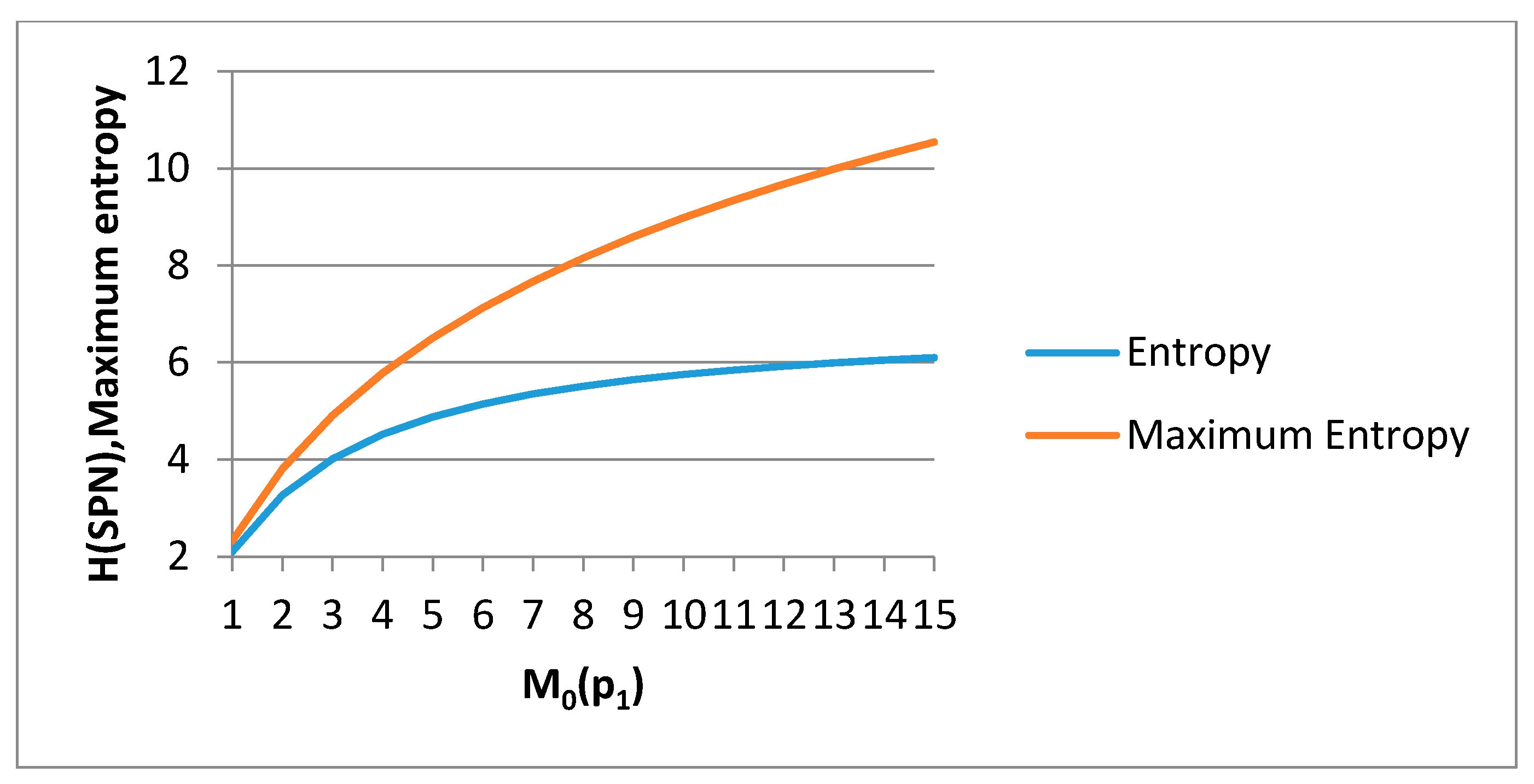Figure 3 shows the evolution of entropy and maximum entropy, depending on the number of tokens in the place p₁. Figure 4 expresses the ratio of the entropy and the maximum entropy from Figure 3, i.e., the uncertainty index, and indicates that the increasing number of tokens in the initial marking (in the place p₁) decreases the uncertainty index of the SPN.

Figure 3. Entropy and maximum entropy vs. number of tokens.

Figure 3. Entropy and maximum entropy vs. number of tokens.

Figure 4. Uncertainty index vs. number of tokens.

Figure 4. Uncertainty index vs. number of tokens.

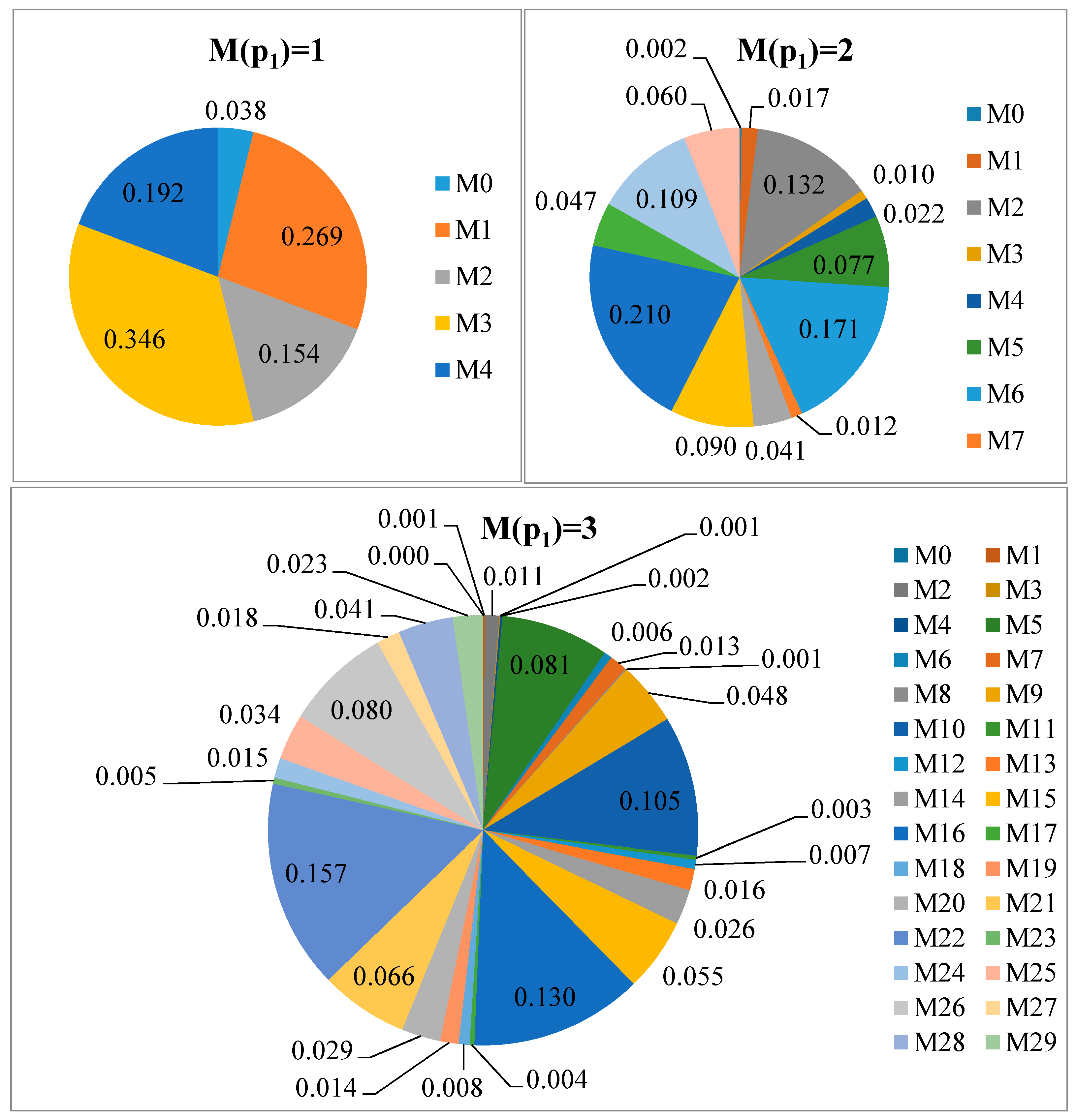
Uncertainty is declining, since for this particular example decreases the uniformity of the stationary probability distribution between markings. This can be verified in the deeper analysis of the distribution of the individual sets of all reachable markings. The stationary probability distribution for various initial marking in the place p₁ is shown in the Figure 5. Increasing the number of tokens in place of p₁, grows the number of reachable markings and also their distribution becomes less uniform, i.e., the overall uncertainty index decreases. Figure 3 and Figure 4 show that the complexity (entropy) is growing, but the uncertainty index decreases.

Figure 5. The stationary probability distribution for various initial marking in the place p₁.

Figure 5. The stationary probability distribution for various initial marking in the place p₁.

If we consider that the example network represents, for instance, the process model for the processing of purchase orders and the number of tokens in place p₁ represents the amount of received purchase orders (in given time), it is possible, based on the values of the uncertainty index, to assess the behaviour of the system, for example, its saturation or robustness. With the increasing number of purchase orders (tokens) the uncertainty index decreases (see Figure 4), i.e., the degree of certainty, that some order is in a particular state grows. This can cause the growth of the average length of the life cycle of the purchase order (e.g., the unprocessed orders can pile up in specific places). In general, different situations may arise, for instance, the average time for the processing of purchase orders may be constant, rise or fall (in different speeds). The manager may consider if the system behaviour conforms (e.g., if it is sufficiently robust to sudden change in the number of purchase orders processed in the same quality). While the behaviour of the system can be influenced by changing the model structure or by modifying its parameters $\mathsf{\Lambda }$. 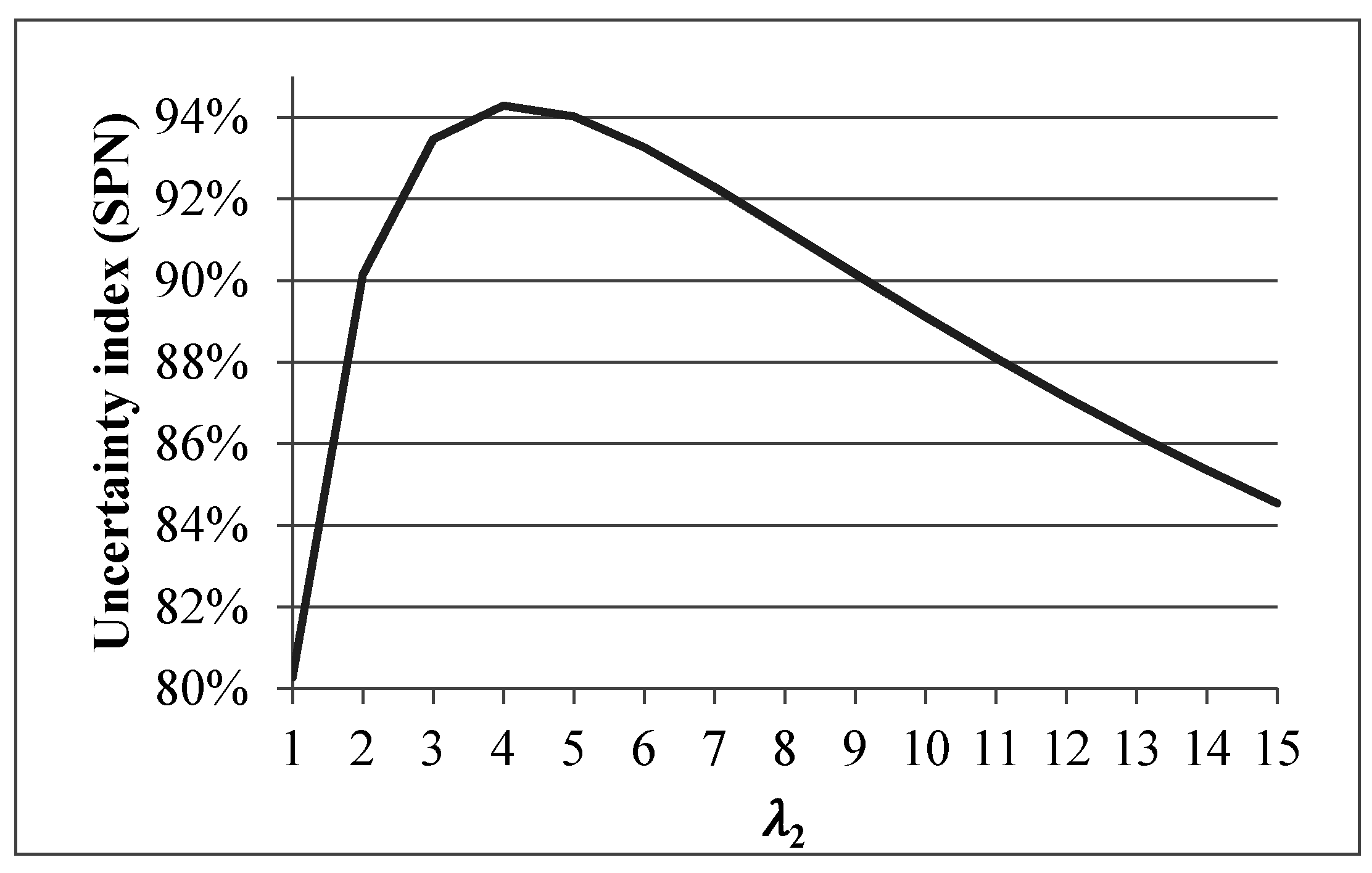Figure 6 shows the evolution of SPN uncertainty index in relation to the changing value of the parameter ${\lambda }_2$. The parameter was selected randomly for the sole purpose of presenting visual analysis capabilities. When considering a fixed number of purchase orders the Figure 6 shows the behaviour of the system when changing the parameter ${\lambda }_2$ (i.e., the time to complete the partial operation with a purchase order; this time can be changed, for instance, by changing the number of workers, better technical equipment of a better organisation of work) and with the conservation of the other parameters values. When the value of ${\lambda }_2$. is equal to 4 the uncertainty index is highest, i.e., the distribution of states (markings) is locally the most uniform (which could be interpreted as a situation that the purchase orders are accumulating in certain places least).

Figure 6. Uncertainty index vs. exponential rate λ₂

Figure 6. Uncertainty index vs. exponential rate λ₂

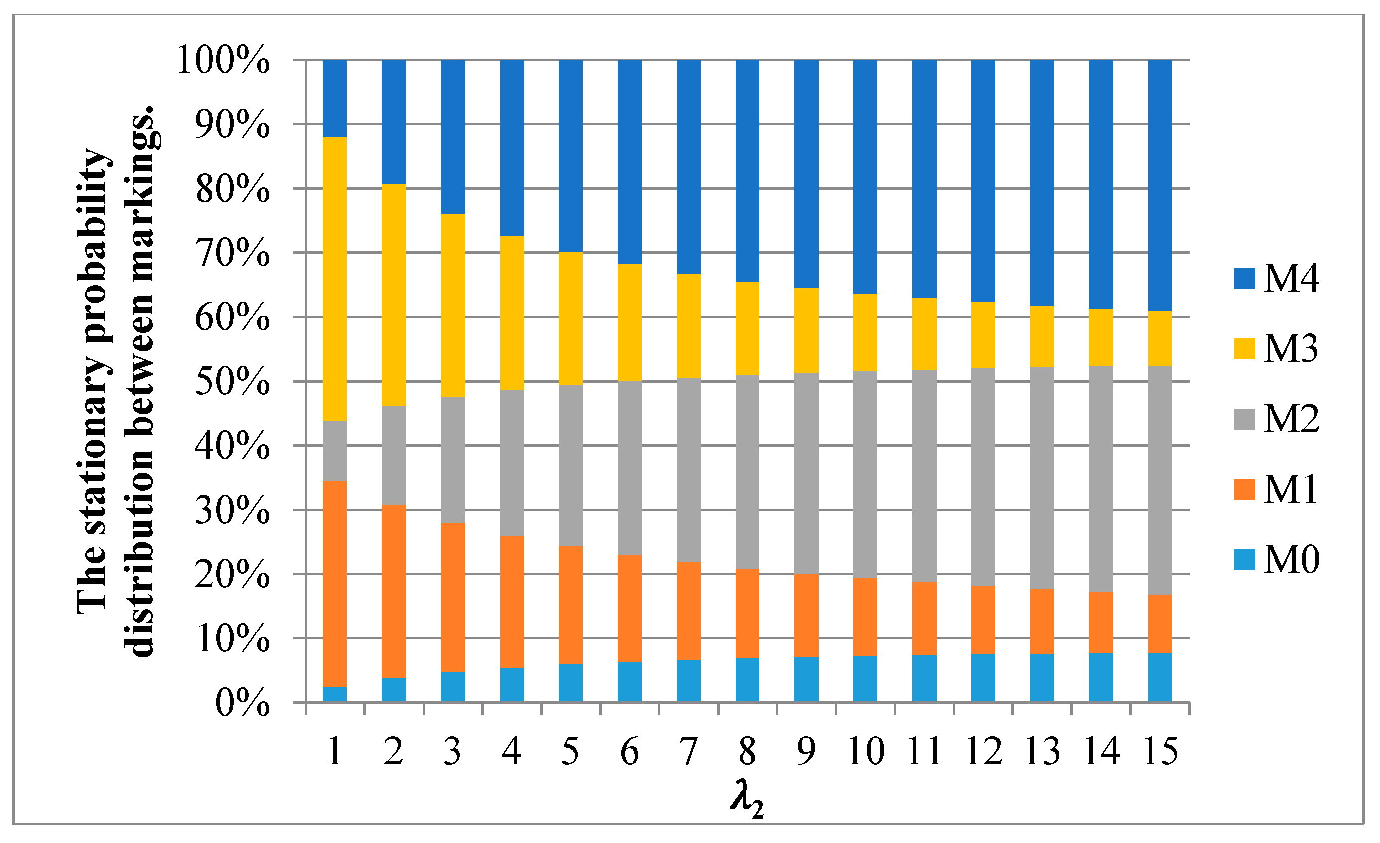
For a better understanding, the relationship between the uncertainty index and changing the exponential parameter ${\lambda }_2$ in the case of $M_0=\left(1,0,0,0,0\right)$ is presented in Figure 7. From the picture, it appears that the increasing value of the parameter ${\lambda }_2$ reduce the dominance of the markings M1 and M3, and enhance the dominance of the markings M2 and M4. When the value of the parameter ${\lambda }_2$is equal to 4, the stationary probability distribution is the most uniform, i.e., the uncertainty index is greatest. In a real application, the change of the parameter $\lambda$ corresponds, for instance, to a variation of the time required for the processing of certain activities (e.g., processing of purchase orders in the example above).

Figure 7. The stationary probability distribution between markings vs. exponential rate 𝜆₂.

Figure 7. The stationary probability distribution between markings vs. exponential rate 𝜆₂.

With this type of analysis is then possible to set different assumptions on the modelled system and assess the behaviour of the system when adjusting various parameters of the model. Interpretability of results is directly linked to the specific problem (specific system that is modelled and analysed). The aim of this article is to present a new approach for the calculation of the uncertainty in stochastic Petri nets, without specific industry applications. This ensures more effective applicability to a broad range of disciplines (logistics, computer network, etc.), without further specialization.

6. Validation

The uncertainty (entropy) can be seen as the complexity of the model, since it reflects properties as the difficulty to understand or maintain the process. According to [14] there are a number of metrics that have been developed over the last few decades, mainly to measure the complexity of software. Most of these metrics can be also used on the issue of business processes. When defining a new metric it is suitable to perform its validation. Validation can be of two types, i.e., the theoretical and empirical validation. One of the most widely used theoretical validation measures is Weyuker’s properties [15]. The Table 1 summarizes the fulfilment or non-fulfilment of each Weyuker’s properties.

Table 1. Fulfilment of Weyuker’s properties for our approach.

	Description	Fulfilment
Property 1	Two different processes should not return the same measurement results	Yes
Property 2	The change in a process should cause a change of its complexity	No
Property 3	It is possible that two distinct processes have the same complexity.	Yes
Property 4	Good metric should discriminate different processes (with the same functionality) based on their internal structure (design)	Yes
Property 5	Complexity of the subprocess should be smaller than or equal to the complexity of the original process.	No
Property 6	It is possible to have two different processes with the same complexity, but if concatenated to a third process, their resulting complexities are not equal.	Yes
Property 7	Complexity should depend on the order of the statements	Yes
Property 8	Renaming of the process or its components does not change its complexity	Yes
Property 9	It is possible that complexity of two interacting processes is bigger than sum of their individual complexities	Yes

Table 1. Fulfilment of Weyuker’s properties for our approach.

	Description	Fulfilment
Property 1	Two different processes should not return the same measurement results	Yes
Property 2	The change in a process should cause a change of its complexity	No
Property 3	It is possible that two distinct processes have the same complexity.	Yes
Property 4	Good metric should discriminate different processes (with the same functionality) based on their internal structure (design)	Yes
Property 5	Complexity of the subprocess should be smaller than or equal to the complexity of the original process.	No
Property 6	It is possible to have two different processes with the same complexity, but if concatenated to a third process, their resulting complexities are not equal.	Yes
Property 7	Complexity should depend on the order of the statements	Yes
Property 8	Renaming of the process or its components does not change its complexity	Yes
Property 9	It is possible that complexity of two interacting processes is bigger than sum of their individual complexities	Yes

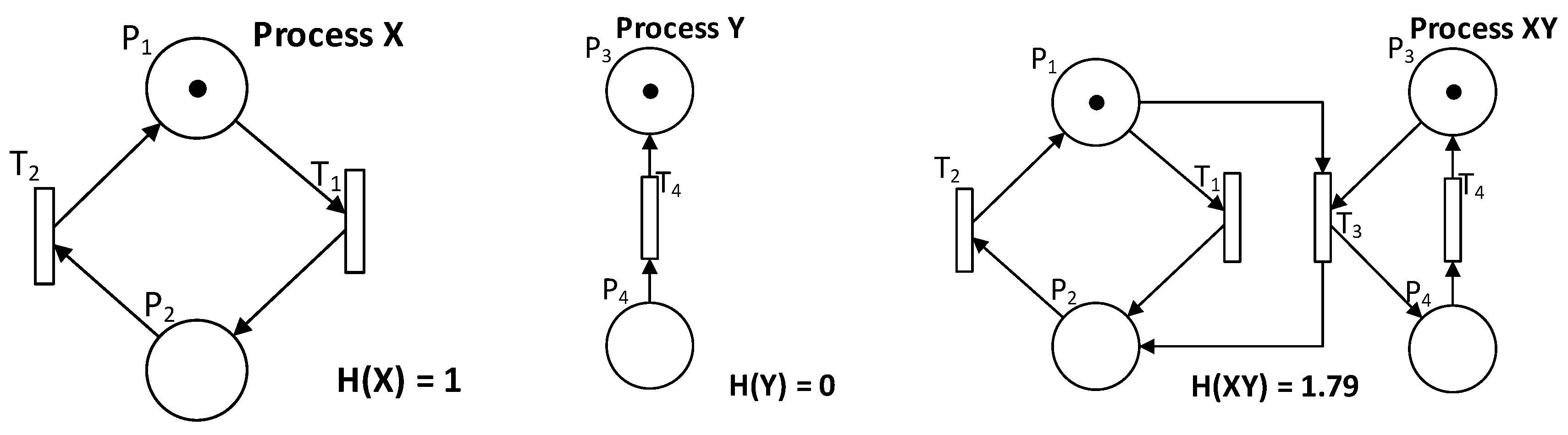
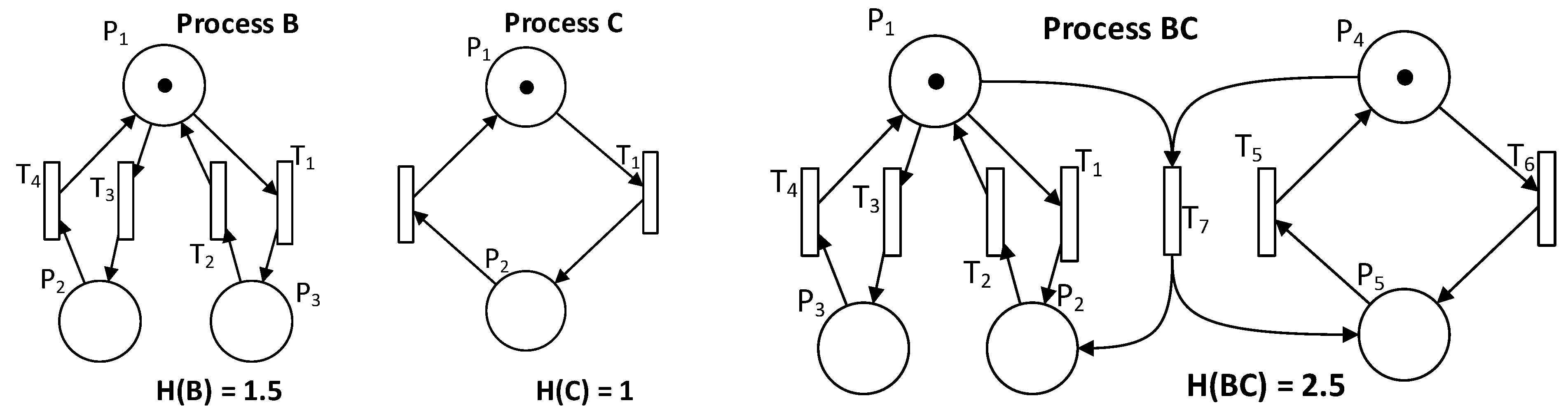
Property 2 is not fulfilled, since there may be an infinite number of Petri nets that have the same underlying Markov chain, i.e., the same complexity (entropy). Concerning property 3, if different Petri nets have the same underlying Markov chain, then they have the same complexity (entropy). Property 5 is not fulfilled, since non-live process, which includes a live subprocess, has the entropy equal to 0, but the complexity of the live subprocess is greater than 0. Property 6 is dependent on the fulfilment of the property 3 and the form of how the two processes are composed together. Figure 8. illustrates the fulfilment of the property 6.

Figure 8. An example for the Property 6 fulfilment.

Figure 8. An example for the Property 6 fulfilment.

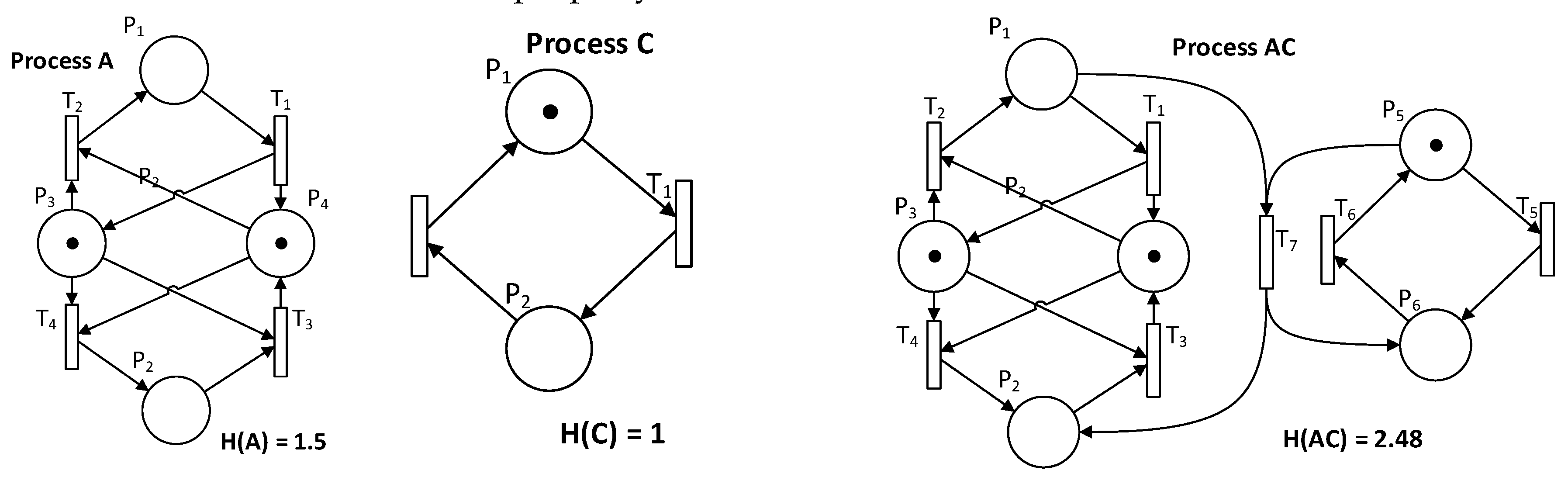
Property 9 is fulfilled, since if a live process is concatenated with a non-live process and the resulting process is live, than the entropy of the resulting process is greater than the sum of individual entropies. An example of the property 9 fulfilment illustrates Figure 9.

Figure 9. An example for the Property 9 fulfilment.

Figure 9. An example for the Property 9 fulfilment.

Further empirical validation was performed (comparison of the existing metrics with our approach). We have made a comparison of the entropy as a complexity measure with the McCabe’s approach [13] and uncertainty-based uncertainty measure introduced in [3]. Table 2 shows the comparison of the resulting values of complexity (our approach, McCabe’s approach and approach introduced in [3]) for the model from Figure 1 (and its modifications).

Table 2. A comparison of the proposed approach with other approaches.

Model	Entropy (Proposed Approach)	McCabe’s Approach [13]	Entropy-Based Uncertainty Measure Introduced in [3]
	2.09	7	4
	1.64	5	2
	1.19	3	2
	0.84	2	0

Table 2. A comparison of the proposed approach with other approaches.

Model	Entropy (Proposed Approach)	McCabe’s Approach [13]	Entropy-Based Uncertainty Measure Introduced in [3]
	2.09	7	4
	1.64	5	2
	1.19	3	2
	0.84	2	0

The table indicates that the resulting values of both approaches show the same trend, i.e., are comparable. The correlation coefficient (based on the presented samples) is 0.996 between our and McCabe’s approach and 0.940 between approach introduced in [3] and ours. The correlation values suggest that there is a strong functional relationship between these approaches (based on the data in Table 2), i.e., they measure the same quantity-complexity.

7. Discussion

Analysis of process models provides valuable information about its usability, predictability and accuracy. One way to quantify the degree of predictability of the process model is using metrics based on the evaluation of uncertainty. Measurement of uncertainty can be an appropriate tool for assessing the relevance and the predictability of these models, and thus serve to more effective managerial decision making. The degree of uncertainty in the process model is directly dependent on two main indicators. The first is the number, the ratio and the distribution of specific elements (OR, XOR, AND, and LOOP) in the model. These elements provide branching, synchronization and cycles in the model, and thus are the main building blocks of process models that shape its specific structure. One of the approaches to the measurement of uncertainty in the process model (defined in [3]) is based on quantifying the entropy of partial substructures of the model at different levels of abstraction. However, this approach takes into account only static structure of the model and does not take into account its dynamic component (behaviour), which can be expressed in Petri nets using tokens. It calculates the uncertainty of the process models that are modelled using Petri nets (puts restrictions on how the model should look like). Our approach uses the value of entropy when comparing models with different structures, plus the index of uncertainty is used when analysing the model when changing its parameters (for instance, initial markings, exponential distribution). The value of the entropy expresses the complexity and the uncertainty index expresses the ratio of the entropy towards the maximum entropy (complexity, which the model can have at most for the same structure, the number of tokens and the exponential distribution). Analysis of the complexity lies in comparing equivalent models (different structure, but the output is the same). The value of uncertainty/complexity (entropy and/or index uncertainty) gives the manager the possibility to change the structure of the model and at the same time to consider the behaviour when changing the model parameters (number of markings representing a specific entity or activity; or the adjustment of the exponential distribution of a transition). On the basis of this analysis, the manager optimizes the process model, to comply with its requirements (structure and behaviour). In other references, for instance [3,14], it is possible to analyse only the structure of the model and not its behaviour. Our approach quantifies the uncertainty of any stochastic Petri net model (the only condition is liveness and boundedness). The second indicator, which implies the uncertainty of process models are branching probabilities in the above-mentioned elements. In the presented method, these probabilities are expressed in the form of firing rates using the exponential distribution for each transition in the network. The structure of the Petri net implies all reachable markings and firing rates imply (using the transition rate matrix) steady-state probabilities of this set. Using the Shannon entropy can be then quantified the level of uncertainty over the Markov chain (reachable markings and their probabilities). The degree of uncertainty (uncertainty index) that is defined on the interval <0,1> can be expressed as a percentage of the calculated entropy against maximum entropy. The resulting value of uncertainty index represents the uniformity of stationary probabilities distribution of individual markings, i.e., the more even distribution of stationary probabilities is, thereby increasing its entropy (approaching the maximum entropy), and at the same time its uncertainty (uncertainty is approaching 100%). The normalization with maximum entropy makes the uncertainty a dimensionless quantity which is suitable for the comparison of models with a different number of reachable markings. Furthermore, it is possible to use the calculated entropy as a measure of complexity, since it meets most of Weyuker’s properties and at the same time, the comparison of our approach with approaches [13] and [3] yields the correlation coefficient of 0.940 and 0.996, respectively.

The advantages of this approach

• The calculation of entropy in the stochastic Petri nets is a universal metric for the evaluation of uncertainty in reactive and concurrent systems. The only restriction is the requirement for modelling using stochastic Petri nets.
• Exactly defined boundaries of uncertainty (interval <0,1>).
• The possibility of using the verification capabilities of Petri nets.
• The possibility of using the entropy as a measure of complexity.
• The possibility to simulate different model parameters (e.g., firing rates, number of tokens), and follow the development of uncertainty index, i.e., the ability to search for local optima within a specific operating point (the original model parameter values).

The disadvantages of this approach

• Standard disadvantages of Petri nets in general, e.g., state explosion (extension of the model with new places or the increase in the number of tokens in the initial marking, leads to an exponential growth of all reachable markings), restrictions based on the definition, etc. Computational efficiency of the uncertainty calculation is directly linked to the number of all reachable markings. Time complexity of the calculation of the stationary probability has the quadratic character (O (N^2), where N is a number of all reachable markings).
• The condition that the model must be live. In other cases, the entropy is equal to zero.
• The condition that the model must be bounded, which ensures that the cardinality of the set of all reachable markings is finite.

There are other approaches that work with uncertainty, for instance [16] use the Dempster Shafer believe theory for modelling uncertainty within Petri and other authors use the fuzzy Petri nets to reduce the uncertainty, for example [17] or [18]. However, none of these approaches is comparable with ours.

8. Conclusions and Future Work

In this work, a procedure for calculation of the uncertainty in stochastic Petri nets has been defined. The level of uncertainty (entropy, uncertainty index) can serve as a useful indicator for determining the degree of predictability in the modelled systems (e.g., process models). The value of entropy is useful when comparing models with different structure and the uncertainty index can be used when analysing the model, i.e., changing its parameters (initial marking, the exponential distribution). The value of entropy expresses the complexity of the model and the uncertainty index expresses the ratio of the entropy to the maximum entropy, i.e., complexity, which the model can have at most for a given structure, the number of tokens and exponential distribution.

On the sample example were presented possible analysis of the SPN model. The evaluation of the theoretical and empirical validation shows that our approach (using entropy to determine the uncertainty in SPN models) is an appropriate approach for measuring complexity in systems modelled using stochastic Petri nets. Future research will focus on the expansion of this approach to the measurement of uncertainty on issues closer to reality. This expansion consists mainly in the diversification of individual tokens. With diversification of tokens can be possibility quantified the uncertainty of complex models. That can be achieved by using, for instance, coloured Petri nets (CPN) that allow us to assign a vector of values as a token.