Supply Chain Strategies for Quality Inspection under a Customer Return Policy: A Game Theoretical Approach

Abstract

This paper outlines the quality inspection strategies in a supplier–buyer supply chain under a customer return policy. This paper primarily focuses on product quality and quality inspection techniques to maximize the actors’ and supply chain’s profits using game theory approach. The supplier–buyer setup is described in terms of textile manufacturer–retailer supply chain where quality inspection is an important aspect and the product return from the customer is generally accepted. Textile manufacturer produces the product, whereas, retailer acts as a reseller who buys the products from the textile manufacturer and sells them to the customers. In this context, the former invests in the product quality whereas the latter invests in the random quality inspection and traceability. The relationships between the textile manufacturer and the retailer are recognized as horizontal and vertical alliances and modeled using non-cooperative and cooperative games. The non-cooperative games are based on the Stackelberg and Nash equilibrium models. Further, bargaining and game change scenarios have been discussed to maximize the profit under different games. To understand the appropriateness of a strategic alliance, a computational study demonstrates textile manufacturer–retailer relation under different game scenarios.

1. Introduction

The supplier–buyer strategic business relation management is an important aspect for both the supplier and the buyer in the supply chain [1]. This is particularly important when the success of one actor in the supply chain is highly dependent on the other. For instance, production outsourcing is one of the contemporary practices followed in the textile industry, where retailers do not own the production facilities and outsource their production activities to various suppliers [2]. Subsequently, the retailers are highly dependent upon the manufacturers for the product quality [3]. Production outsourcing helps the retailers in terms of reduced risk by not owning the production facilities and the reduced production cost since the manufacturer are located in countries where cheap labor is available, however, at the same time creates other responsibilities including proper quality inspection of the supplier-delivered products. Due to the increased manufacturer/supplier–retailer distance, the retailer cannot observe the production activities at a distantly located supplier. Further, there exist uncertainties in the supply chain associated with the demand, delivery time and customer requirements, which relate to the performance of the supply chain [4]. As supplier and retailer may have divergent priorities in terms of investment in production quality, this gives an advantage as well as the malicious opportunity to the suppliers to provide defective or inferior products to the retailer [5]. In this context, the responsibility of the retailer is to implement an optimal quality inspection strategy to minimize or avoid the risks associated with defective products.

Quality inspection helps in identifying the defective or non-conforming items or supplies provided by a supplier. However, as all the product characteristics are difficult to inspect due to technological and financial constraints, there is always a possibility of defective products reaching the end-user customer [3]. In such events, it is important for the retailer to provide a fair compensation on product returns (such as product repair, replacement, discount, etc.) to ensure the confidence of customers [6,7,8]. Furthermore, the financial liabilities associated with the above-mentioned product return-based compensations have prompted practitioners and researchers to reassess the quality inspection policies and share the defective product borne liabilities with the supplier who is the originator of the defect.

With the increasing importance of quality inspection aspect, many researchers have explored the potential of different supply chain practices. Cheng et al. [3] described inspection measures in two categories: ex-ante and ex-post. Ex-ante includes the traditional quality inspection techniques where the supplier and retailer formulate a quality contract and the retailer inspects the supplies by random inspection methodology. The effect of quality/inspection policies with/under inventory policies [9], penalties [10], rewards, joint lot sizing [11,12], return policies [8,13], uncertain demand [14] and ordering policies [15] on supply chain contracts have been discussed. Heish and Liu [5] have discussed the optimal investment in quality and inspection activities with different degrees of information revealed among the manufacturer and supplier.

More recently, increasing attention has been paid to traceability-based ex-post quality inspection techniques [3,16,17]. Traceability-based ex-post inspection extends the quality inspection perspective beyond the point of supply transaction and any quality-related issue can be traced back at any stage of the product lifecycle using the traceability information. One of the primary reasons for the move toward ex-post inspection is the limitation associated with traditional inspection-based contracts (ex-ante), which provide an opportunistic prospect for malfeasance by the supplier due to the imperfect inspection techniques and expenses [3]. The extended quality inspection by traceability-based ex-post quality inspection is particularly important for textile products which have a large number of quality characteristics, and measuring them is not only time-consuming, but technologically and monetarily expensive [3,18]. Subsequently, it is more effective for the retailer. According to GS1 Global Traceability System [19], traceability is defined as “the ability to track forward the movement through specified stage(s) of the extended supply chain and trace backwards the history, application or location of that which is under consideration.” Therefore, any quality-related issues identified beyond the point of supply transaction (where ex-ante inspection ends) can be traced back to its origin. Studies to approach different business objectives using traceability have been discussed in the past. For the food and agribusiness, traceability has been discussed in relation with safety, recalls, inventory management and other related aspects including quality management system, product and process history [10,16,17,20,21]. Cheng et al. [3] explored traceability for optimizing supply chain quality from a textile supply chain perspective.

The textile sector has also seen a large transformation arising due to several factors, including migration of the industry towards certain countries resulting in complex supply chains, and the emergence of concepts like fast fashion, which has significantly reduced the fashion lifecycle. Further, there are a number of uncertainties associated with market demands, changing product variety, the rate of product innovation, production lead-time, delay in logistics delivery, failure of firms to deliver the product or raw material, etc. [22]. In addition, issues like vendor-managed inventory are a general concern for supply chain management [23]. Concerning this, Christopher et al. [24] addressed the fashion market as a system with a high level of “chaos”. Supply chain actors are becoming more collaborative to plan the strategies to minimize different risks and uncertainties, and improving the efficiency of the supply chain [4]. According to Martino et al. [25], the first step to manage the various risks associated with such a chaotic supply chain is to analyze the internal processes to isolate the most relevant weakness factors. In this context, quality is a key competitive factor in the textile industry, however, it is attained as a result of successive quality management strategies implemented at different levels in the supply chain [3,18]. Generally, a supply chain actor will be willing to invest in producing a better product or a quality inspection system (or any other context) as long as it benefits him directly or indirectly. Furthermore, the investment and benefits are also affected by the relation with the other actors in the supply chain. Several researchers have identified the supply chain management factors affecting the quality of products [26] and have quantified the benefits of product quality or related investments in terms of profit, using different relationships with other supply chain members and associated uncertainties [3,5,8,14]. In the context of quality inspection strategies, most of the literature has either focused on random quality inspection based ex-ante techniques [7,27,28] or traceability-based ex-post techniques [10,17]. Furthermore, limited attention has been paid to combining these techniques simultaneously with different supply-chain dynamics (such as power asymmetries and cooperation between the supply chain actors). Nevertheless, Cheng et al. [3] illustrated the optimization of a fashion supplier–manufacturer chain with inspection control and traceability control methodologies.

Thus, this article aims to demonstrate the appropriateness of simultaneously implementing a conventional random quality inspection (ex-ante) technique and a recently emerged traceability-based (ex-post) technique in the supply chain using a game theory approach. The objective is to maximize the profits of supply chain actors considering different power asymmetries in the supply chain, which covers a research gap observed in the literature.

Here the focus is given to a textile manufacturer–retailer relation under product return policy using game theoretic approach, where the textile manufacturer and retailer try to maximize their respective profits by controlling investments in production and quality inspection (ex-ante and ex-post), respectively. Retailers in a supply chain act as a link between the final consumer and the manufacturer/supplier [29]. Retailers act as “gatekeepers”, determining the market demands and placing orders with the manufacturer [30]. For a given cost of the product paid by the retailer to a textile manufacturer, the textile manufacturer’s main objective is to maximize his profit by minimizing the investment in production (or product quality). Whereas, the retailer would like to have maximum product quality so that he has a less product returns. Moreover, the retailer also considers opting for random inspection policy and traceability. Random quality inspection allows filtering of non-conforming products received from the textile manufacturer, whereas traceability ensures that if a consumer reports a fault or returns the product, the retailer can identify the textile manufacturer to penalize him. Traceability has in fact recently highlighted the necessity for the retailers from various perspectives including warehouse management, supply chain visibility, safety, security, product recalls and economic incentives associated traceability information [17,31]. In the textile supply chain, a retailer is often associated with multiple suppliers for different types of product. Therefore traceability helps the retailer to identify the manufacturer of different products [32].

The subsequent parts of the paper are organized as follows: Section 2 describes our model framework. Section 3 describes the textile manufacturer–retailer relations in four different game scenarios, among which three (two Stackelberg games and one Nash game) are non-cooperative, and one is a cooperative game scenario. Section 4 discusses the suitability of different game models from the textile manufacturer’s and retailer’s perspectives, the possibility of bargaining and forced cooperation among the actors for the profit maximization. Section 5 demonstrates a numerical example for illustrating the models. Finally, Section 6 concludes this paper and provides suggestions for future research.

2. Model Framework

According to Surana et al. [33], “A supply chain is a complex network with an overwhelming number of interactions and inter-dependencies among different entities, processes and resources.” Present global supply chain networks consist of numerous enterprises linked together through a complex interplay of products and services, consistently work to improve the supply chain effectiveness and decision making to sustain an advantage against the competition generated by growing number of industries [34,35]. In this context, mathematical models coupled with behavior and organizational theories provide a sound framework for practices and decision-making in complex networks of collaborating enterprises [27,28,29,30]. Since the supply chain consists of multiple enterprises integrated by some common goals but having different constraints and conflicting objectives, these enterprises can be seen as players in a game [36,37,38].

We use a game theory approach to analyze the relationship between the textile manufacturer and the retailer. The model used in this paper is based on supplier-buyer relation under constant demand used in the past [27,28,39]. It should be noted that in the supply chain literature, the terms vendor, seller, supplier, and manufacturer have been used interchangeably to represent the manufacturer. Similarly, the terms retailer, buyer, and distributor have been used to represent the retailer. To avoid ambiguity in this paper we use the terms textile manufacturer and retailer. The model assumes three components of the supply chain, namely textile manufacturer, retailer, and customer, which is similar to that of used in the literature (e.g., [3,16,17,28]). The textile manufacturer serves the retailer and the retailer serves the end-use customer. As proposed in the literature, a customer’s buying preference is influenced by multiple factors, including product quality, product specification, brand value, trends, and services such as product return policies and traceability where the customer can trace back the product and raw material history [40,41]. In light of constant demand and price assumptions, we neglect the factors such as brand preference and trend. In order to counterbalance any quality-related issues, we assume the retailer provides fair compensation to the customer so the customer comes back to the retailer in future and maintains a constant demand. Further, we assume traceability as a tool for the retailer to identify the textile manufacturer, not a tool for consumers to know the product history. Therefore, the level of traceability does not affect the customer or product quality. Furthermore, the retailer accepts all product returns in case of a defect; however, we treat the probability of return by a customer as an exogenous function. It should be noted that when only one textile manufacturer and one retailer are involved in the supply chain, it is obvious that the retailer can fully identify the textile manufacturer in the case of a product return, without needing to use any traceability. In practice, multiple textile manufacturers may serve a single retailer (e.g., the Swedish clothing brand H&M has ~750 suppliers [42]). Therefore, traceability helps in identifying which particular product belongs to which supplier. In this paper, we represent the same situation by one retailer and one textile manufacturer (also considered in a similar way in the literature e.g., [17]), where the retailer has a certain probability s to identify the textile manufacturer and then there is a 1 − s probability that the retailer cannot identify the textile manufacturer.

2.1. Assumptions

In order to reduce the complexity we make the following assumptions in the proposed textile manufacturer–retailer relation:

• All the actors are rational.
• All parameters are deterministic and known in advance.
• Demand and market price functions $\left(I_1,I_2,I_3\right)$ are constant. Although the demand and product quality are related to each other but we assume that retailer provides enough compensation to satisfy the consumer when the consumer reports a faulty/non-conforming product. Following Ref. [17], we assume $I_1>I_2>I_3$.
• Production quality, random quality inspection level and traceability level are controllable and follow their respective cost functions (i.e., $C_p(P)$ and $C_{Qs}(Q,s)$) (also used in the literature, cf. [3]).
• Return of the product is applicable to the faulty products, which were sold as a good product by the retailer. The return rate i.e., probability of a product return is an exogenous function.
• The retailer can accept a faulty product but cannot reject a non-faulty/conforming product to the textile manufacturer.
• Both actors should individually make a positive profit to remain in the game.

The remaining assumptions are described in the text when they appear.

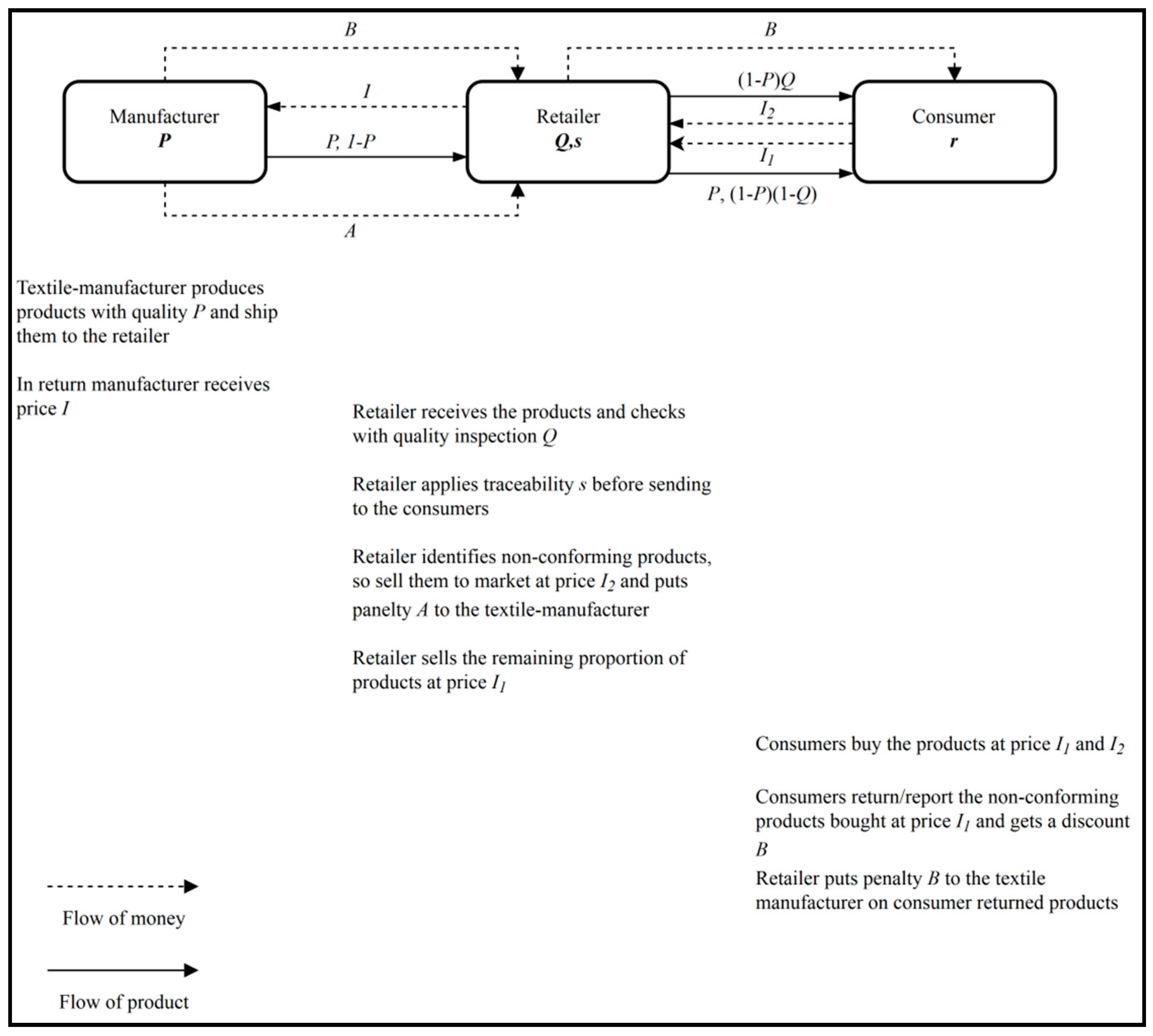
2.2. Textile Manufacturer–Retailer Interaction

We assume that the textile manufacturer knows how to produce a retailer-ordered conforming product and the production cost follows a production cost function $C_p(P)$, where P is the probability that the product produced by the manufacturer conforms to the retailer’s requirements. The production cost function is an increasing concave function, i.e., $C_p(•)>0,C_p^{\prime }(•)>0,C_p^{″}(•)>0$. Similar to [3,43], we chose the production cost functions in the form $C_p(P)={\alpha }_p+\frac{1}{2}{\beta }_p{P}^2$.

After receiving the shipment from the textile manufacturer, the retailer invests in random quality inspection and traceability. The retailer firstly inspects the received product and generates an appraisal by quality inspection, Q, where Q represents the probability that the retailer identifies a product as non-conforming. Similar to reference [3], it is assumed that the retailer can commit Type-I errors, i.e., he may not identify a non-conforming product as conforming, but cannot commit Type-II errors, i.e., he cannot appraise a conforming product as non-conforming. As it is well acknowledged in the literature that for the textile products it is rather difficult to monitor or measure all the quality characteristics due to technological or cost constraints [3,44], therefore there exists a probability of Type-I error. Nevertheless, the identified non-conforming products are sold in the market at a lower market price ($I_2$) than that of conforming product ($I_1$). In order to recover the loss caused by a non-conforming product, the retailer penalizes the textile manufacturer. For rationality, the retailer sets the penalty cost as A, where $A=I_1-I_2$, therefore, retailer earns the same selling price (i.e., $I_2+A$) as for a conforming product (i.e., $I_1$). Selling faulty textiles at a lower price is the general practice in the textile supply chain where retailer may remove the retailer’s/brand’s identification marks such as logos and labels from garments and then sell them at a lower price. By selling faulty textiles as a generic garments (i.e., without any brand information), retailer/brand owner protects himself from a negative brand image.

Further, as mentioned above, since the retailer can commit Type-I errors, there is a certain probability that he cannot identify all the non-conforming inbound products. In this context, the retailer invests in traceability implementation so that he can identify the manufacturer if a consumer returns a non-conforming product that has escaped the quality inspection. Here traceability, s, is defined as the probability that the retailer can identify the manufacturer, i.e., $0\le s\le 1$, as defined by [17]. Further, to protect the brand value, the retailer gives a discount B (so the net selling price is $I_3=I_1-B$) to the customer to satisfy the consumer and places a penalty (B) on the textile manufacturer to recover the loss because of the discount.

As discussed by [3] the quality inspection and traceability implementation cost to the retailer follow an increasing concave function. Therefore we use, $C_{Qs}(Q,s)=\left({\alpha }_Q+{\beta }_Q\frac{Q^2}{2}\right)+\left({\alpha }_s+{\beta }_s\frac{s^2}{2}\right)$, $({\alpha }_Q,{\alpha }_s,{\beta }_Q,{\beta }_s)>0$ such that $C_{Qs}(•)>0,\frac{\partial C_{Qs}(•)}{\partial Q}>0,\frac{\partial C_{Qs}(•)}{\partial s}>0,\frac{{\partial }^2{C}_{Qs}(•)}{{\partial }^{2}Q}>0,\frac{{\partial }^2{C}_{Qs}(•)}{{\partial }^{2}s}>0$, hence $C_{Qs}(Q,s)$ is an increasing concave function.

The textile manufacturer–retailer relation is shown in Figure 1. A list of the nomenclature used in this paper is shown in

Table 1. Notations.

Notation	Description
A, B	Penalty costs to the textile manufacturer for the non-conforming products identified in random quality inspection and traceability respectively
$C_p(P),C_{Qs}(Q,s)$	Cost functions for implementing product quality (P), and quality inspection techniques (Q, s) respectively
I	The price per product charged by the manufacturer to the retailer
$I_1$	Selling price charged by the retailer to the consumer
$I_2$	Selling price of non-conforming product identified by the retailer
$I_3$	Net selling price of the non-conforming/defected product identified by the consumer
K	Coefficient deciding the profit proportion of the follower
P	Product quality rate, as proportion of product that succeed to meet the retailer’s quality requirement or conformation, $0\le P\le 1$
Q	Random quality inspection rate, as the proportion of nonconforming products detected in quality inspection, $0\le Q\le 1$
r	Return rate, as the proportion of the non-conforming product returned by the consumer. $0\le r\le 1$
s	Traceability success rate, as the proportion of the return successfully identified by the retailer to the manufacturer. $0\le s\le 1$
${\alpha }_P,{\beta }_p$	Coefficients related to cost function $C_p(P)$
${\alpha }_Q,{\alpha }_s,{\beta }_Q,{\beta }_s$	Coefficients related to cost function $C_{Qs}(Q,s)$
$\gamma$	Factor related to relative bargaining power of the textile manufacturer and the retailer
${\Pi }_{TM}$	Manufacturer’s profit per product
${\Pi }_R$	Retailer’s profit per product
$\Pi$	Total supply chain profit, $\Pi ={\Pi }_{TM}+{\Pi }_R$

Superscripts TM, R, N and C have been used with the above parameters to represent that they belong to the Stackelberg’s textile manufacturer game, the Stackelberg’s retailer game, the Nash game and cooperative game, respectively.

.

2.3. Textile Manufacturers Model Formulation

The textile manufacturer’s objective is to maximize his profit by investing in product quality P to minimize the penalty from non-conforming products. Similarly, the product cost i.e., I is decided by the textile manufacturer to maximize his profit. Based upon the discussion in the last section, the following textile manufacturer’s objective function, ${\Pi }_{TM}$, can be formulated:

$${\Pi }_{TM}=I-\underset{x}{\underbrace{\left(1-P\right)QA}}-\underset{y}{\underbrace{\left(1-P\right)\left(1-Q\right)srB}}-C_p\left(P\right)$$

(1)

where the term denoted by x represents the penalty cost to the textile manufacturer imposed by the retailer for the non-conforming products identified during the retailer’s random quality inspection, and y represents the penalty cost to the textile manufacturer imposed by the retailer for traceable non-conforming products returned by the consumer. The division of the product into various components is shown in

Table 2. Description of various components’ division during product flow.

Sr. No.	Description	Proportion
1	Proportion of good products among total produced products	P
2	Proportion of non-conforming products among identified in retailer’s random quality inspection	$\left(1-P\right)Q$
3	Proportion of traced non-conforming products which were not identified in retailer’s random quality inspection but returned by the consumer	$\left(1-P\right)\left(1-Q\right)sr$
5	Proportion of non-conforming products which were not identified in retailer’s random quality inspection and also did not return by the consumer	$(1-P)(1-Q)(1-r)$
6	Proportion of non-traceable non-conforming products which were not identified in retailer’s random quality inspection but returned by the consumer	$(1-P)(1-Q)(1-s)r$
	Total	1.0

.

Since $\frac{{\partial }^2{\Pi }_{TM}\left(P\right)}{\partial P^2}<0$ therefore ${\Pi }_{TM}$ can be maximized for a fixed value of I by applying the first-order condition to Equation (1) i.e.,

$$\begin{gathered} \frac{\partial {\Pi }_{TM}(P)}{\partial P^2}=0 \\ \Rightarrow P^{\ast }=\frac{QA+\left(1-Q\right)srB}{{\beta }_P} \end{gathered}$$

(2)

It should be noted that * denotes the optimum parameter.

According to the condition $0\le P\le 1$, Equation (2) can be written as:

$$P^{\ast }=\min \left\{1,\frac{QA+\left(1-Q\right)srB}{{\beta }_P}\right\}$$

(3)

Further, as it can be seen in Equation (1) that ${\Pi }_{TM}$ is linear function of I, the value of I (denoted by $I_0$) that results to ${\Pi }_{TM}$ = 0 can be calculated as:

$$I_0=\left(1-P\right)QA+\left(1-P\right)\left(1-Q\right)srB+C_p\left(P\right)$$

(4)

According to assumption vii, every actor needs to make a non-zero positive profit for a successful contract. Hence, $I>I_0$ or $I=K{I}_0$ where K is >1 [45]. Therefore the optimum I can be calculated as:

$$I^{\ast }=K\left\{(1-P)QA+(1-P)(1-Q)srB+C_p(P)\right\}$$

(5)

2.4. Retailer’s Model Formulation

Retailer’s objective to maximize his profit by optimizing his random quality inspection and traceability. Retailer’s objective function can be formulated based upon Figure 1 as:

$$\begin{array}{r}{\Pi }_R\left(Q,s\right)=\{P+(1-P)(1-Q)(1-r)\}{I}_1+(1-P)Q(I_2+A)+(1-P)(1-Q)sr(I_3+B)+\\ (1-P)(1-Q)(1-s)r{I}_3-I-C_{Qs}(Q,s)\end{array}$$

(6)

${\Pi }_R\left(Q,s\right)$ is a concave function w.r.t. s for a fixed Q (since ${\partial }^2{\Pi }_R\left(s,Q\right)/\partial s^2$ $=-{\beta }_s$ < 0), therefore the value of s that maximizes Equation (6) can be calculated by applying the first-order condition to Equation (6) w.r.t. s, i.e.,

$$\frac{\partial {\Pi }_R}{\partial s}=0\Rightarrow s\left(Q\right)=\frac{r(1-P)(1-Q)B}{{\beta }_s}$$

(7)

Similarly, ${\Pi }_R\left(s,Q\right)$ is a concave function w.r.t. Q for a fixed s (since ${\partial }^2{\Pi }_R\left(s,Q\right)/\partial Q^2$ $=-{\beta }_s$ < 0), therefore the value of Q that maximizes Equation (6) can be calculated by applying the first-order condition to Equation (6) w.r.t. Q, i.e.,

$$\frac{\partial {\Pi }_R}{\partial Q}=0\Rightarrow Q\left(s\right)=\frac{(1-P)(1-s)rB}{{\beta }_Q}$$

(8)

Further, optimum values of Q and s can be calculated by plugging Equation (7) into Equation (8) and then solving for Q and s:

$$s^{\ast }=\frac{{\beta }_{Q}r(1-P)B-r^2{(1-P)}^2{B}^2}{{\beta }_Q{\beta }_s-r^2{(1-P)}^2{B}^2}$$

(9)

$$Q^{\ast }=\frac{{\beta }_{s}r(1-P)B-r^2{(1-P)}^2{B}^2}{{\beta }_Q{\beta }_s-r^2{(1-P)}^2{B}^2}$$

(10)

To follow the conditions i.e., $0\le Q\le 1$ and $0\le s\le 1$, Equations (9) and (10) can be rewritten as:

$$s^{\ast }=\{\begin{array}{cc}0,& if({\beta }_Q\zeta -{\zeta }^2)({\beta }_s{\beta }_Q-{\zeta }^2)<0\\ 1,& if\frac{{\beta }_Q\zeta -{\beta }_s{\beta }_Q}{{\beta }_s{\beta }_Q-{\zeta }^2}>0\\ \frac{{\beta }_Q\zeta -{\zeta }^2}{{\beta }_s{\beta }_Q-{\zeta }^2},& else\end{array}$$

(11)

$$Q^{*}=\{\begin{array}{cc}0,& if({\beta }_s\zeta -{\zeta }^2)({\beta }_s{\beta }_Q-{\zeta }^2)<0\\ 1,& if\frac{{\beta }_s\zeta -{\beta }_s{\beta }_Q}{{\beta }_s{\beta }_Q-{\zeta }^2}>0\\ \frac{{\beta }_s\zeta -{\zeta }^2}{{\beta }_s{\beta }_Q-{\zeta }^2},& else\end{array}$$

(12)

where, $\zeta =r(1-P)B$.

Additionally, the supply chain profit $\Pi$ can be calculated by adding the individual profits of textile manufacturer i.e., ${\Pi }_{TM}$ from Equation (1) and that of the retailer i.e., ${\Pi }_R$ from Equation (6), given as:

$$\begin{array}{r}\Pi ={\Pi }_{TM}+{\Pi }_R=\{P+(1-P)(1-Q)(1-r)\}{I}_1+(1-P)Q{I}_2+(1-P)(1-Q)sr{I}_3+\\ (1-P)(1-Q)(1-s)r{I}_3-C_{Qs}(Q,s)-C_P(P)\end{array}$$

(13)

3. Formulation of Game Scenarios

Game theory is one of the most widely used tools employed in the past to analyze situations involving conflict and cooperation [38,46]. In the textile supply chain, there exists a dynamic field of conflicting and cooperative objectives in the supplier-retailer relation [30]. Cooperation is described as a favored situation benefitting the whole supply chain [30,47], however, when the conflicting interests of actors outweigh the cooperating interests, the supply chain efficiency is reduced [48]. Recently, with the increased level of outsourcing, buyer firms are placing more emphasis on the relations with the suppliers, hence moving towards more cooperative scenarios [49]. In the case of textile manufacturer–retailer relations, the power is often skewed toward either of the parties. For instance, big retailers placing big orders are often able to exert power on smaller suppliers to reduce prices [50]. Therefore, in the quest to achieve higher profit coupled with power dominance, the retailers tend to move away from cooperation [51]. Although, a non-cooperative contract may help the power-dominating player earn more profit, the overall profit of the supply chain is hindered [30]. Such a relationship can be termed as a vertical alliance between a leader and a follower. When both the parties involved in a contract have equal power and both target their strategies simultaneously at maximizing their profits, the relation again moves away from cooperation to a polarized non-cooperating game [38]. When the actors, either cooperatively decide a strategy to maximize the profit of the supply chain (cooperative game), or simultaneously and non-cooperatively set their strategies to maximize the own profits, their alliance in the contract can be termed as a horizontal alliance. In the latter case, both actors act as “supply chain captains”, working toward their profit whereas in the former case, none of the actors acts as supply chain captain.

In the light of scenarios discussed above, we discuss the textile manufacturer–retailer relation in two types of games namely, non-cooperative and cooperative games. The non-cooperative game has three cases depending upon the dominance of the actors i.e., dominant textile manufacturer (Stackelberg’s textile manufacturer game), dominant retailer (Stackelberg’s retailer game) and both having equal power (Nash game).

3.1. Non-Cooperative Games

In this section, we model various relations between the textile manufacturer and retailer in the non-cooperative way, i.e., an actor in the textile manufacturer–retailer network works toward optimizing his own profit. The non-cooperative games are discussed in the three following scenarios.

3.1.1. The Stackelberg’s Textile Manufacturer Game

In the Stackelberg’s textile manufacturer game, the textile manufacturer is power dominant and acts as leader, while the retailer acts as a follower. The leader has absolute power to maximize his profit while leaving the follower with the minimum profit needed to retain him in the contract [38,52]. Therefore, firstly the textile manufacturer takes the retailer’s controlled optimum parameters i.e., Q and s then adjusts his own controlled parameters i.e., P and I so that the textile manufacturer maximizes his profit. As can be seen in Equation (1), the textile manufacturer’s profit ${\Pi }_{TM}$ is a linearly increasing function of I, where the manufacturer keeps on increasing I to maximize his profit and leave the retailer with zero profit i.e., ${\Pi }_R=0$. I for ${\Pi }_R=0$ (denoted by $I_0$) can be written as:

$$\begin{array}{r}{I}_0=\{P+(1-P)(1-Q)(1-r)\}{I}_1+(1-P)Q(I_2+A)+(1-P)(1-Q)sr(I_3+B)+\\ (1-P)(1-Q)(1-s)r{I}_3-C_{Qs}(Q,s)\end{array}$$

(14)

According to assumption vii, every actor needs to have a non-zero positive profit for a successful contract. Therefore, we take $I<I_0$ or $I=\frac{I_0}{K}$ where K > 1, which results ${\Pi }_R>0$.

Further, the textile manufacturer’s objective function can be written as:

$$\underset{P,I}{\max }{\Pi }_{TM}=I-\left(1-P\right)QA-\left(1-P\right)\left(1-Q\right)srB-C_p\left(P\right)$$

(15)

subject to:

$$0\le P\le 1$$

(16)

$$s=\{\begin{array}{cc}0,& if({\beta }_Q\zeta -{\zeta }^2)({\beta }_s{\beta }_Q-{\zeta }^2)<0\\ 1,& if\frac{{\beta }_Q\zeta -{\beta }_s{\beta }_Q}{{\beta }_s{\beta }_Q-{\zeta }^2}>0\\ \frac{{\beta }_Q\zeta -{\zeta }^2}{{\beta }_s{\beta }_Q-{\zeta }^2},& else\end{array}$$

(17)

$$Q=\{\begin{array}{cc}0,& if({\beta }_s\zeta -{\zeta }^2)({\beta }_s{\beta }_Q-{\zeta }^2)<0\\ 1,& if\frac{{\beta }_s\zeta -{\beta }_s{\beta }_Q}{{\beta }_s{\beta }_Q-{\zeta }^2}>0\\ \frac{{\beta }_s\zeta -{\zeta }^2}{{\beta }_s{\beta }_Q-{\zeta }^2},& else\end{array}$$

(18)

$$I=\left[\begin{array}{r}\{P+(1-P)(1-Q)(1-r)\}{I}_1+(1-P)Q(I_2+A)+(1-P)(1-Q)sr(I_3+B)+\\ (1-P)(1-Q)(1-s)r{I}_3-C_{Qs}(Q,s)\end{array}\right]/K$$

(19)

It should be noted that the subscript TM is used with the above-optimized parameters in later sections (i.e., $P^{TM},I^{TM},s^{TM},Q^{TM}$) to represent the optimized parameters during the comparison with the other game scenarios.

3.1.2. The Stackelberg’s Retailer Game

In this game scenario, we model a retailer-dominated textile manufacturer–retailer relation using the Stackelberg’s retailer game model. The retailer has absolute power to maximize his profit while leaving the textile manufacturer with the minimum profit to retain him in the contract. Therefore, firstly the retailer takes the textile manufacturer controlled optimum parameters i.e., P and I then adjusts his own controlled parameters i.e., Q and s so that the retailer maximizes his gains. Therefore, the retailer’s objective maximization problem can be written as:

$$\begin{array}{r}\underset{Q,s}{\max }{\Pi }_B=\{P+(1-P)(1-Q)(1-r)\}{I}_1+(1-P)Q(I_2+A)+(1-P)(1-Q)sr(I_3+B)+\\ (1-P)(1-Q)(1-s)r{I}_3-I-C_{Qs}(Q,s)\end{array}$$

(20)

subject to:

$$0\le Q\le 1$$

(21)

$$0\le s\le 1$$

(22)

$$P=\min \left\{1,\frac{QA+\left(1-Q\right)srB}{{\beta }_P}\right\}$$

(23)

$$I=K\left\{(1-P)QA+(1-P)(1-Q)srB+C_P(P)\right\}$$

(24)

3.1.3. The Nash Game

In this section, we follow the Nash game model to formulate a textile manufacturer-retailer game model where both the actors non-cooperatively and simultaneously maximize their own profits on their own. Therefore, in this game, we have two objective functions to maximize with the following conditions:

$$\begin{array}{r}\underset{Q,s}{\max }{\Pi }_R=\{P+(1-P)(1-Q)(1-r)\}{I}_1+(1-P)Q(I_2+A)+(1-P)(1-Q)sr(I_3+B)+\\ (1-P)(1-Q)(1-s)r{I}_3-I-C_{Qs}(Q,s)\end{array}$$

(25)

subject to:

$$0\le Q\le 1,0\le s\le 1$$

(26)

and:

$$\underset{P,I}{\max }{\Pi }_{TM}\left(P,I\right)=I-\left(1-P\right)QA-\left(1-P\right)\left(1-Q\right)srB-C_P\left(P\right)$$

(27)

subject to:

$$0\le P\le 1$$

(28)

As can be seen from Equation (27) ${\Pi }_{TM}$ is a linear function of I, thus the textile manufacturer will obtain his maximum profit by increasing with a value of I which obviously leaves the retailer with a zero profit. Similarly, ${\Pi }_R$ is a negative linear function of I (Equation (25)) thus to maximize ${\Pi }_R$ the retailer needs to have the minimum possible value of I which will obviously leave the textile manufacturer with zero profit. In this conflicting scenario, we incorporate a hypothesis as used in Ref. [52,53]: if the textile manufacturer and the retailer make their decisions simultaneously then they both receive equal margin so that both the parties get equal profit, i.e., ${\Pi }_{TM}={\Pi }_R$, which results in:

$$I=\frac{1}{2}\left[\begin{array}{r}\{P+(1-P)(1-Q)(1-r)\}{I}_1+(1-P)Q(I_2+2A)+(1-P)(1-Q)sr(I_3+2B)+\\ (1-P)(1-Q)(1-s)r{I}_3-C_{Qs}(Q,s)+C_P(P)\end{array}\right]$$

(29)

The optimum Q and s have been solved for ${\Pi }_R$ in Equations (11) and (12), and P has been solved for ${\Pi }_{TM}$ Equation (3). Thus the Nash equilibrium can be obtained by the following parameters:

$$P^N=\{\begin{array}{cc}0& if({\beta }_{Q}rB-{\xi }^2)({\beta }_P{\beta }_Q-{\xi }^2)<0\\ 1& if\frac{{\beta }_{Q}rB-{\beta }_P{\beta }_Q}{{\beta }_P{\beta }_Q-{\xi }^2}>0\\ \frac{{\beta }_{Q}rB-{\xi }^2}{{\beta }_P{\beta }_Q-{\xi }^2}& otherwise\end{array}$$

(30)

$$Q^N=\{\begin{array}{cc}0& if(\xi ({\beta }_P-rB))({\beta }_P{\beta }_Q-{\xi }^2)<0\\ 1& if\frac{\xi ({\beta }_P-rB)}{{\beta }_P{\beta }_Q-{\xi }^2}>1\\ \frac{\xi ({\beta }_P-rB)}{{\beta }_P{\beta }_Q-{\xi }^2}& otherwise\end{array}$$

(31)

$$s^N=0$$

(32)

where $\xi =\left(rB-A\right)$.

3.2. Cooperative Game

In this section, we formulate a cooperative game model where both the actors work together to maximize the whole supply chain’s profit. The whole supply chain’s profit is given in Equation (13) and the controlling parameters in the supply chain are P, Q, and s. It should be noted that the internal payment function I controls the profit of individual players, but the whole supply chain profit is independent of I. Moreover, the proportion of profit division depends on the bargaining power of each actor [52]. The supply chain objective function can be written as:

$$\begin{array}{r}\underset{P,Q,s}{\max }\Pi =\{P+(1-P)(1-Q)(1-r)\}{I}_1+(1-P)Q{I}_2+(1-P)(1-Q)sr{I}_3+\\ (1-P)(1-Q)(1-s)r{I}_3-C_{Qs}(Q,s)-C_P(P)\end{array}$$

(33)

subject to:

$$0\le P\le 1$$

$$0\le Q\le 1$$

$$0\le s\le 1$$

Taking the first order derivative of Equation (33) w.r.t. P, Q and s, we get the following:

$$\frac{\partial \Pi }{\partial P}=QA+(1-Q)rB-{\beta }_{P}P$$

(34)

$$\frac{\partial \Pi }{\partial s}=-{\beta }_{s}s$$

(35)

$$\frac{\partial \Pi }{\partial Q}=(1-P)(rB-A)-{\beta }_{Q}Q$$

(36)

Thus the optimum values of P, Q and s can be calculated by applying first-order conditions on Equations (34)–(36), respectively, i.e.,

$$P=\frac{1}{{\beta }_P}\left(QA+(1-Q)rB\right)\ge P^{\ast }$$

(37)

$$s=0\le s^{\ast }$$

(38)

$$Q=\frac{(1-P)(rB-A)}{{\beta }_Q}$$

(39)

Proposition 1.

The textile manufacturer needs to invest more on quality at a given return rate for the cooperative game as compared to that of the Stackelberg’s retailer non-cooperative game. Traceability remains at the lowest level in a cooperative game.

Proof. 

As it can be seen, Equation (37) ≥ Equation (23), which means for a given r, P in the cooperative game is equal to or more than P in the Stackelberg’s retailer game. Similarly, s = 0 for all r as can be seen in Equation (38), therefore traceability remains at the lowest level in the cooperative game. Hence the proposition is proved.

The optimum parameters, i.e., $P^C$and $Q^C$can be obtained by simultaneously solving Equations (37) and (39) while taking into account $0\le P^C,Q^C\le 1$. Solving these equations would lead to the solution given in Equations (31) and (32), thus ${\Pi }^C={\Pi }^N$ .

The individual profits of retailer and textile manufacturer depend on I, i.e., the internal payment, which depends on the mutual agreement. In order to have a mutual agreement, both the players should have a higher profit than in any alternate game. For instance, the textile manufacturer will agree to a cooperative game only if ${\Pi }_{TM}^C>\max \left({\Pi }_{TM}^R,{\Pi }_{TM}^{TM},{\Pi }_{TM}^N\right)$ i.e., the textile manufacturer’s profit is higher in the cooperative game as compared to that of a non-cooperative game. Similarly, the retailer will agree to a cooperative game only if ${\Pi }_R^C>\max \left({\Pi }_R^R,{\Pi }_R^{TM},{\Pi }_R^N\right)$ i.e., the retailer’s profit is higher in the cooperative game as compared to that of a non-cooperative game. The possibility of a cooperative game is discussed in the subsequent sections.

4. Bargaining Feasibility and Game Change Scenarios

4.1. Game Change and Bargaining

Bargaining between the textile manufacturer and retailer is possible in a cooperative game where both the actors agree to work together to maximize the supply chain profit, and both benefit from the increased profit. As mentioned in Section 3.2, the profit of an individual actor depends upon the bargaining power of each actor, since I, which is one of main parameters affecting the profit, is an independent parameter. Furthermore, parties will agree on cooperation if and only if their profits are more than with other games [52,54]. For instance, for the Stackelberg’s textile manufacturer game, the textile manufacturer is the main player who decides the profit. Therefore, a textile manufacturer can bargain with a retailer for a cooperating game if:

$$\Delta {\Pi }^{TM}(r)={\Pi }^C(r)-{\Pi }^{TM}(r)>0$$

(40)

It should be noted that the r in parentheses above denotes the parameters for a given return rate r. Here $\Delta {\Pi }^{TM}(r)$ denotes the supply chain’s surplus profit when the textile manufacturer changes from a non-cooperating game to a cooperating game for a given return rate r. Therefore, the textile manufacturer can bargain with the retailer to go to a cooperative game and share the profit $\gamma \Delta {\Pi }^{TM}$, where $0\le \gamma \le 1$. If the retailer accepts the cooperating game then the retailer gets overall profit ${\Pi }_R^C(r)={\Pi }_R^{TM}(r)+\gamma \Delta {\Pi }^{TM}(r)$, whereas the textile manufacturer gets profit ${\Pi }_{TM}^C(r)={\Pi }_{TM}^{TM}(r)+(1-\gamma )\Delta {\Pi }^{TM}(r)$. The factor $\gamma$ depends on the relative bargaining power of the textile manufacturer and the retailer. When $\gamma =0.5$ both the textile manufacturer and the retailer share the surplus profit equally, whereas for $\gamma <0.5$, the manufacturer is dominating and if $\gamma >0.5$ the retailer is dominating in bargaining. For $\gamma >1$, ${\Pi }_{TM}^C(r)<{\Pi }_{TM}^{TM}(r)$ or for $\gamma <0$, ${\Pi }_B^C(r)<{\Pi }_B^{TM}(r)$ hence the cooperative game is not feasible.

Similarly, for the Stackelberg’s retailer game, surplus profit ($\Delta {\Pi }^R(r)$) from changing from a non-cooperative to a cooperative game can be written as:

$$\Delta {\Pi }^R(r)={\Pi }^C(r)-{\Pi }^R(r)$$

(41)

when $\Delta {\Pi }^R(r)>0$, the profits in the cooperative game can be written as:

$${\Pi }_R^C(r)={\Pi }_R^R(r)+\gamma \Delta {\Pi }^R(r)$$

(42)

$${\Pi }_{TM}^C(r)={\Pi }_{TM}^{TM}(r)+(1-\gamma )\Delta {\Pi }^R(r)$$

(43)

4.2. Competition among Non-Cooperative Games

Non-cooperative games aim to maximize the profit an actor without cooperating with the other actor. As aforementioned, in the case of Stackelberg games, the leader tries to get maximum profit and shares the minimum profit with the follower to retain him in the game. However, in the case of the Nash game, both the actors act non-cooperating with each other and try to simultaneously and non-cooperatively maximize their profits. The benefit of latter over former game is that none of the parties has to bother about other party to retain in contract since both are gaining the equal profit as long as the contract exists i.e.,

$${\Pi }_{TM}^N(r)={\Pi }_R^N(r)=\frac{{\Pi }^N(r)}{2}$$

(44)

Therefore, the change in game from the Stackelberg’s textile manufacturer game is possible when, $\frac{{\Pi }^N(r)}{2}>\max \left({\Pi }_{TM}^{TM},{\Pi }_R^{TM}\right)$, such that ${\Pi }_{TM}^N(r)>{\Pi }_{TM}^{TM}(r)$ and ${\Pi }_B^N(r)>{\Pi }_B^{TM}(r)$. In the changed game (i.e., from the Stackelberg’s textile manufacturer to the Nash game), the textile manufacturer remains non-cooperating while the retailer changes from an adherent to non-cooperative, and both gain higher profit than that of the former game. Similarly, for the Stackelberg’s retailer game scenario, the retailer (as dominant) will agree to switch the game if $\frac{{\Pi }^N(r)}{2}>\max \left({\Pi }_{TM}^R(r),{\Pi }_R^R(r)\right)$.

4.3. Forced Game Change and Cooperation

The benefit of becoming the leader in the game theory is having extreme power and getting the opportunity to maximize gain [51]. However from this power follows the responsibility that the leader should provide minimum incentives to the follower to keep him in the contract. Therefore, an actor in the supply chain would like to be the leader as long as he gains more profit than with alternate games scenarios (such as a cooperating game or as follower in the non-cooperating game). Assuming for case of textile manufacturer, the textile manufacturer would like to be the leader for a given return rate as long as:

$${\Pi }_{TM}^{TM}(r)\ge \max \left({\Pi }_{TM}^C(r),{\Pi }_{TM}^R(r)\right)$$

(45)

Similarly, for the case of retailer, the retailer would like to be the leader as long as:

$${\Pi }_R^R(r)\ge \max \left({\Pi }_R^C(r),{\Pi }_R^{TM}(r)\right)$$

(46)

However, for the scenario with a given return rate r, ${\Pi }_R^R(r)<\max \left({\Pi }_R^C(r),{\Pi }_R^{TM}(r)\right)$ and ${\Pi }_{TM}^{TM}(r)<\max \left({\Pi }_{TM}^C(r),{\Pi }_{TM}^R(r)\right)$ both the actors would like to change the game and since nobody would like to be the leader, the only solution to settle an optimum profit is a cooperative game, which is the common choice for both actors.

In the case of ${\Pi }_R^R(r)<\min \left({\Pi }_R^{TM}(r),{\Pi }_R^C(r)\right)$ and ${\Pi }_{TM}^{TM}(r)\ge {\Pi }_{TM}^R(r)$, it is better for the retailer to either participate in a cooperation game or a follower game (Stackelberg textile manufacturer game). The Stackelberg’s textile manufacturer game is favorable when ${\Pi }_{TM}^{TM}(r)>{\Pi }_{TM}^C(r)$ or a cooperative game is favorable when ${\Pi }_{TM}^C(r)>{\Pi }_{TM}^{TM}(r)$. In the above two games, no cooperative game is possible when $\Delta {\Pi }^B(r)<{\Pi }_{TM}^{TM}(r)-{\Pi }_{TM}^B(r)$.

Similarly, when ${\Pi }_{TM}^{TM}(r)<\min \left({\Pi }_{TM}^B(r),{\Pi }_{TM}^C(r)\right)$ and ${\Pi }_B^B(r)\ge {\Pi }_B^{TM}(r)$, it is better for the textile manufacturer to participate either in the cooperative game or a Stackelberg’s retailer game. The Stackelberg’s retailer game is favorable when ${\Pi }_B^B(r)\ge {\Pi }_B^C(r)$ or the cooperative game is favorable when ${\Pi }_B^C(r)>{\Pi }_B^B(r)$. In two above games, no cooperative game is possible when $\Delta {\Pi }^{TM}(r)<{\Pi }_B^B(r)-{\Pi }_B^{TM}(r)$.

5. Results and Discussion

In this section, we provide numerical examples to calculate the various parameters for maximizing profits under different established game scenarios and locate the best strategies for different return rates. We select the following parameters for the demonstration, $I_1=250$, A = 70 ($I_2=I_1-A=180$), B = 150 ($I_3=I_1-B=100$), ${\alpha }_s={\alpha }_Q=30$, ${\beta }_s={\beta }_Q=80$, ${\alpha }_P=50$, ${\beta }_P=150$, K = 1.3.

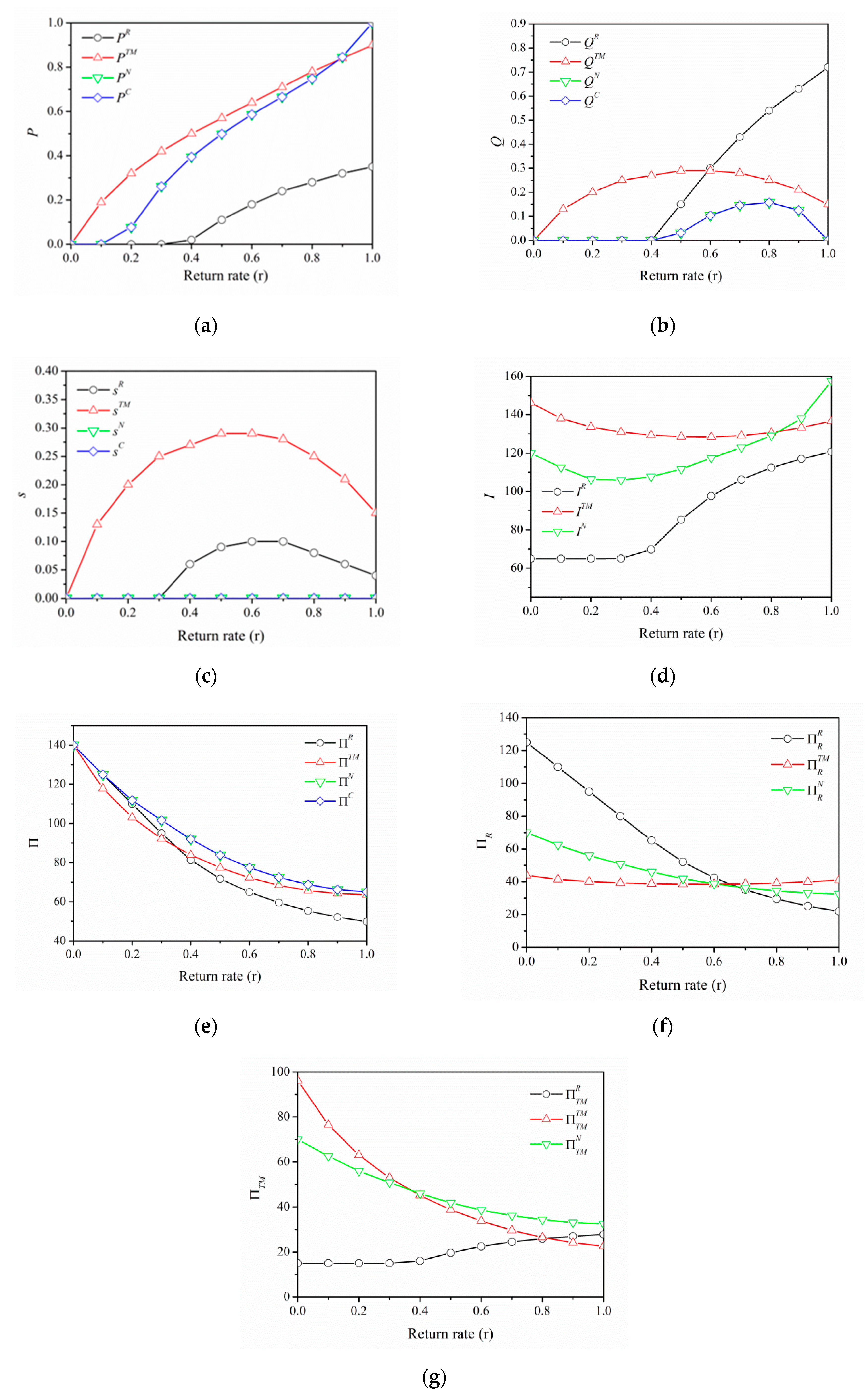
Graphical results corresponding to the abovementioned parameters are shown in Figure 2. Except for a very high return rate, the textile manufacturer’s product quality remains high for a textile manufacturer-dominated game (P^TM) whereas it remains lowest for the retailer-dominated game (P^R) (Figure 2a). The retailer’s quality inspection Q remains at the lowest level for r < 0.4 for all the games except textile manufacturer-dominated (Q^TM) game (Figure 2b). Traceability remains at the lowest level for the games where there is no single supply chain captain (i.e., either both are cooperative (s^C) or both are non-cooperative (s^N)), whereas the traceability level in the manufacturer-dominant game (s^TM) exceeds that in a retailer-dominatant game (s^R) (Figure 2c). Nevertheless, non-zero traceability confirms that companies should invest on traceability when the two actors are non-cooperating in the supply chain. Figure 2d shows the change in internal transfer payment I for different game scenarios with varying return rate (r).

As the return rate increases, the supply chain profit ($\Pi$) of all the games reduces (as seen in Figure 2e). This is due to the fact that with the increase in return rate, the probability of defective products being returned by the customer is higher and thus profit is being lost in the form of compensation. Higher return rates can be expected for expensive products, therefore if a firm is trying to obtain higher profit by inflating the product price, the simultaneous increase in return rate might have the opposite effect, as seen in a decrease in profit due to higher return rates. Also, the whole supply chain profit is highest in the cooperative game $\left({\Pi }^C\right)$ as compared with the Stacketberg’s textile manufacturer and the Stacketberg’s retailer games. For non-cooperative games, the order of supply chain profit changes with return rate i.e., for $r<0.35$ ${\Pi }^N\ge {\Pi }^R\ge {\Pi }^{TM}$, and for $r\ge 0.35$ ${\Pi }^N\ge {\Pi }^{TM}\ge {\Pi }^R$ .

Figure 2f,g show the changes in individual profits of actors in different game scenarios. As a common observation, the leader’s profit in all the games goes down as the return rate increases. The leader has to provide a fixed profit (defined by parameter K) to the follower to retain him in the contract [45,55]. Based upon the follower’s investment, the profit varies in all the games. For example, textile manufacturer’s profit in the Stackelberg’s retailer game increases with the increase in return rate, whereas the retailer’s profit in the Stackelberg’s textile manufacturer game initially decreases and then increases.

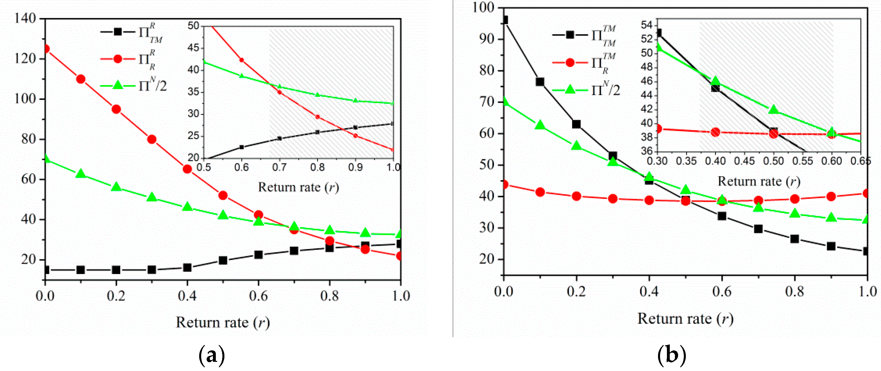
Figure 3 shows the variation of profit under different non-cooperating game scenarios. There is a region for the retailer to switch to the Nash game from a retailer-dominated game as shown by the shaded region in Figure 3a, i.e., $r>0.67$. Similarly, for the textile manufacturer-dominated game, it is profitable for the manufacturer to go into the Nash game with the retailer for $0.33\le r\le 0.6$ (shown by shaded region in Figure 3b). Changing from a non-cooperative game to a cooperative game is always possible since ${\Pi }^C\ge \max \left({\Pi }^R,{\Pi }^{TM},{\Pi }^N\right)$. Actors in a cooperation game work like strategic partners, working toward a common goal [45,56]. Therefore agreement among the actors is an important aspect for its success [49]. 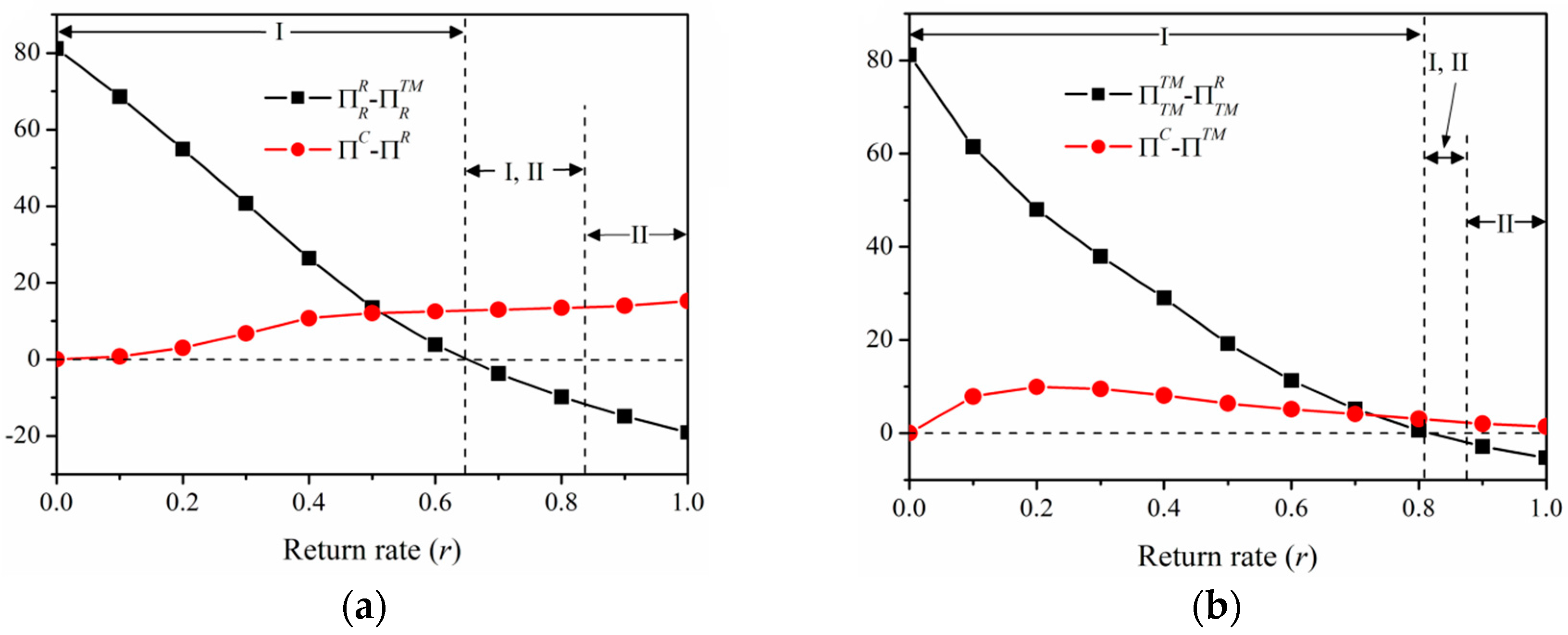Therefore, the changing from a non-cooperative game to a cooperative game depends on a common incentive such as profit sharing and other contractual terms [52]. Looking into the profit scenarios of each player individually, the retailer (as a leader in Stackelberg’s game) would like to lead the game as long as he is getting a high profit [52,54]. Since $\Delta \Pi ={\Pi }^C-{\Pi }^R\ge 0\forall r$ (Figure 4a) therefore the retailer has the possibility to change the game from Stackelberg’s retailer to cooperating game as long as he gains a higher profit, i.e., ${\Pi }_R^C\ge {\Pi }_R^R$.

For this scenario, both actors should agree to a profit division such that ${\Pi }_R^C={\Pi }_R^R+\gamma \Delta \Pi$ and ${\Pi }_{TM}^C={\Pi }_{TM}^R+(1-\gamma )\Delta \Pi$. However, the retailer as a leader would prefer to switch to the follower position when he gains more profit as a follower [54]. For instance, when $r>0.65$, retailer as a follower earns more profit than as a leader, because ${\Pi }_R^R-{\Pi }_R^{TM}<0\forall r>0.65$. Therefore, there are two profit-maximizing ways, one is either to switch to a cooperating game or to switch to a follower game. Depending upon the bargaining power [52], i.e., $\gamma$ retailer can maintain his profit equal to or more than that in Stackelberg’s textile manufacturer game for $0.65<r\le 0.83$. For $r>0.83$, $\Delta \Pi ={\Pi }^C-{\Pi }^B<0$, therefore, the only option left for the retailer to maximize his profit is switch to a game as a follower. In fact, for $0.65<r\le 0.81$, ${\Pi }_{TM}^{TM}-{\Pi }_{TM}^R>0$ therefore the textile manufacturer would agree to be the leader in the game as his profit increases. Different game regions are denoted by I (Cooperative) and II (follower in Stackelberg’s game) in Figure 4a.

Similarly, for the Stackelberg’s textile manufacturer game, cooperative is profitable for $r\le 0.81$, cooperative or follower in Stackelberg’s textile manufacturer game for $0.81<r\le 0.87$ and follower in Stackelberg’s textile manufacturer game $r>0.87$. Comparing the two scenarios (Figure 4a,b), for $r>0.81$ none of the actors wants to lead the game. Therefore, the only option left for both is forced cooperation, where both share the profit or loss equally.

In the abovementioned game models, the return rate was assumed to be an exogenous function. However, it can be compared with a changing business environment. For instance, with the easy accessibility of the Internet, a customer can educate himself with the product return policies or share a product defect on social media that can attract the attention of other users who bought the same product and hence encourage its return. Therefore, the changed business environment seen in terms of high return rate may force the organizations to rethink their business strategies as demonstrated by the appropriateness of different alliances (horizontal/vertical with leader/follower).

6. Conclusions

In this paper, we have discussed the supply chain strategies for quality inspections incorporating the effect of customer return policy using different game models. The textile manufacturer invests in the product quality whereas retailer invests in the random quality inspection and traceability. The maximum supply chain profit was obtained when both actors cooperate in the supply chain. Further, the proposed work shows that the change of roles in non-cooperative game strategies is possible under special circumstances which increase the profits of both actors.

The present work assumes that complete information about each other is available to both the actors. By excluding this assumption, future research can be focused on asymmetric information where incomplete information is available. Furthermore, the effect of product quality, traceability information, and variable penalty cost can be included in the market demand for the future work. The role of chaos arising from uncertainties caused by factors such as market demand and trend changes can be explored using Parraondo’s Paradox game [57].