Predicting the Outcome of NBA Playoffs Based on the Maximum Entropy Principle

Abstract

Predicting the outcome of National Basketball Association (NBA) matches poses a challenging problem of interest to the research community as well as the general public. In this article, we formalize the problem of predicting NBA game results as a classification problem and apply the principle of Maximum Entropy to construct an NBA Maximum Entropy (NBAME) model that fits to discrete statistics for NBA games, and then predict the outcomes of NBA playoffs using the model. Our results reveal that the model is able to predict the winning team with 74.4% accuracy, outperforming other classical machine learning algorithms that could only afford a maximum prediction accuracy of 70.6% in the experiments that we performed.

1. Introduction

The National Basketball Association (NBA), the highest level basketball league in the world, was founded in 1946, and has had a 70 year history. NBA games are now among the most professional, marketed, attended, in addition to being one of the most popular leagues in the world. The NBA enjoys a big following around the world, with many participants anticipating results, in addition to a multitude of betting companies offering vast amounts of money to gamblers on odds of one team winning against another [1,2]. Most participants often place their odds subjectively based on their personal preference of teams without any scientific basis, thus accuracy of the prediction is often very poor. With the rapid advance in science and technology, specifically using sophisticated data mining and machine learning algorithms, forecasting the outcome of a game with high precision is highly feasible and of great economic significance to various players in the betting industry.

By 1950, the popularity of the NBA had increased globally, necessitating the need to forecast results of NBA games; thus, experts began to focus on the historical records of game statistics in a bid to turn the data into useful information. In the early days, most researchers just applied simple principles of statistics that simply combined technical features of past games to create a ranked list of teams used to forecast likelihood of a home team winning an upcoming game [3,4]. However, their accuracy is low compared to probabilistic based machine learning methods. As data for past games became more ubiquitous, researchers began to look for more methods to apply to the large amounts of data; thus, a vast amount of articles related to the analysis and forecasting of results of sports encounters were published. With advances in statistics and processing power of personal computers, researchers leveraged this power to improve accuracy in prediction. Bhandari et al. [5] developed the Advanced Scout based on a Windows personal computer machine in 1996, which pushed NBA games’ data into data mining and the knowledge discovery technology field, and enabled coaches to find some interesting patterns of the competition of basketball games based on data.

By the end of the 20th century, scientists started using a variety of machine learning algorithms to forecast NBA games. Existing research that has used neural nets and decision trees has a major limitation of limited datasets, which lead to overfitting of both models. Consequently, the models will perform very well based on the training data but very low based on the test dataset [6,7,8]. The Maximum Entropy model overcomes this limitation by making use of little known facts and making no assumptions about the unknown. Similarly, the support vector machine is limited by its failure to output a probability value, but only a win or loss, which makes the results difficult to explain [9]. Lack of independence between some features used in sports forecasting is a major limitation to research, such as [10], that uses the Naive Bayes method.

Recently, many scholars have used a variety of probability graph models to simulate games [11,12,13], and their results are promising. However, their major focus is the difference between the simulation and the real game, but not to predict the final outcome of the game. They also do not compute their prediction accuracy. Stekler et al. [14] examined some different evaluation procedures and compared prediction accuracy of some forecasting methods. Haghighat et al. [15] reviewed the use of data mining technologies (neural nets, support vector machines, Bayesian method, decision trees and fuzzy system) to forecast the results of sports events and evaluated the advantages and disadvantages of each method. However, they did not evaluate the Maximum Entropy method, and, to the best of our knowledge, this is the first piece of research to apply the Maximum Entropy model to sports forecasting.

The Maximum Entropy model is more concerned about the construction of feature functions and the preprocessing of feature values of the data. In this paper, using the Maximum Entropy principle, we attempt to overcome the feature independence assumption that limits the Naive Bayesian model. We apply the Maximum Entropy principle to a set of features and establish the NBA Maximum Entropy (NBAME) model. Then, we use the model to calculate the probability of the home team’s win of an upcoming game and make predictions based on this probability. Our results show that the prediction accuracy is pretty high when compared with other machine learning algorithms.

The rest of this paper is arranged as follows: in the following sections, we describe the Maximum Entropy model and k-means clustering. Section 3 gives an overview of the NBAME model. Section 4 presents the experiment results and compares them with results from other algorithms. Finally, concluding remarks and suggestions for future work are given in Section 5.

2. Background

Before exploring the use of the entropy-based scheme in NBA predication, we discuss the Maximum Entropy model, and the k-means clustering algorithm, which we used to discretize continuous valued attributes.

2.1. Maximum Entropy Model

The concept of “information entropy” dates way to 1948 when Shannon [16] first put forward the concept of information entropy. Information entropy is the expected value of information contained in a message. As a measure of random events’ uncertainty, information entropy can explicitly be written as

$$H(p)=-\sum _{i=1}^n{p}_{i}log(p_i),$$

(1)

where $H(p)$ is the information entropy, and $p_i$ is the probability of the ith random event.

Jayne [17] proposed a criterion that was subject to precisely stated prior data, and the probability distribution which best represents the current state of knowledge is the one with the largest entropy. This criterion is known as the “Maximum Entropy principle”. The Maximum Entropy principle points out the best approximation to unknown probability distribution, which satisfies any constraints on the unknown distribution that we are aware of and makes no subjective assumptions about unknown conditions. In this case, the probability distribution is most uniform, and the risk of making a wrong prediction is at the lowest level.

The Maximum Entropy model, also known as a log-linear model, is based on the Principle of Maximum Entropy. Unlike the Naive Bayes classifier, the Maximum Entropy model does not assume that the features are conditionally independent of each other. The Maximum Entropy approach is superior to similar approaches in many circumstances [18,19], especially when the number of samples is small [20]; this is partly because it is not only a regression approach but also its optimization routine is guaranteed to converge on the Maximum Entropy solution.

In recent years, Maximum Entropy based models have been widely used for Natural Language Processing (NLP) tasks, especially for tagging sequential data [21,22,23]. These models have a great advantage over traditional Hidden Markov Models (HMMs) and Naive Bayes models. For example, the Maximum Entropy models can incorporate richer features in a well-founded fashion that HMMs do not. Maximum Entropy based models have also been widely applied to many areas lately: (1) Tseng and Tuszynski [24] gave several examples of applications of Maximum Entropy in different stages of drug discovery; (2) Xu et al. [25] proposed a continuous Maximum Entropy method to investigate the robust optimal portfolio selection problem for the market with transaction costs and dividends; and (3) Phillips et al. [26] studied the problem of modeling the geographic distribution of a given animal or plant species by maximum-entropy techniques. Since the Maximum Entropy model is designed to solve the problems for cases that have insufficient information, we argue that it may provide a very appropriate approach to NBA playoffs prediction.

2.2. K-Means Clustering

Like many supervised machine learning algorithms, the Maximum Entropy model requires a discrete feature space. In order to train the Maximum Entropy model with a very limited training dataset, we need to convert attributes that have continuous numeric values into discrete ones. There has been a lot of research done on continuous feature discretization field [27,28,29,30,31,32]. Methods for discretization are broadly classified into Supervised vs. Unsupervised, Global vs. Local, and Static vs. Dynamic. Recursive minimal entropy partitioning, the error based discretization and Self Organized Map (SOM) based discretization are several supervised discretization processes [33]. However, unsupervised methods do not make use of class labels for discretization. Equal width binning is one of the simplest approaches to the unsupervised discretization process, together with equal frequency binning [34]. Other methods based on the clustering principles include k-means clustering discretization [35].

Jain [36] provided an overview of clustering algorithm development and application. k-means clustering is a method of vector quantization and is originally from signal processing. The standard algorithm was first proposed by Lloyd in 1982 [37], and its main concept is to partition n observations $\{x_1,x_2,···,x_n\}$ into k clusters, in which each observation belongs to the cluster with the nearest mean.

Algorithmic steps for k-means clustering:

• Let $\{x_1,x_2,···,x_n\}$ be the set of data points and $V=\{v_1,v_2,···,v_c\}$ be the set of centers;
• Randomly select “c” cluster centers and calculate the distance between each data point and cluster centers;
• Assign the data point to the cluster center whose distance from the cluster center is the minimum of all the cluster centers;
• Recalculate the new cluster center using: $v_i=(1/c_i){\sum }_{j=1}^{c_i}{x}_i$, where $c_i$ represents the number of data points in ith cluster;
• Recalculate the distance between each data point and new obtained cluster centers;
• If no data point was reassigned, then stop; otherwise, repeat from step 3.

Nowadays, k-means clustering is very popular, and one of the most effective unsupervised discretization algorithms [38] in the data mining field [39,40,41], and this motivated our decision to use it to discretize our feature values. Kanungo et al. [42] presented a simple and efficient implementation of the k-means clustering algorithm.

3. Materials and Methods

In this section, we describe basic technical features of each game and apply the Maximum Entropy principle to build the NBAME model.

3.1. Basic Technical Features

We formalized the “outcome predicting” problem as a two class classification problem. Each game is described by a vector consisting of 29 features of participating teams and the outcome of the game (the label).

Table 1. Basic technical features used by the model.

Feature	Abbreviation	Feature	Abbreviation
Field Goal Made	FGM	Field Goal Attempt	FGA
Three Point Made	3PM	Three Point Attempt	3PA
Free Throw Made	FTM	Free Throw Attempt	FTA
Offensive Rebounds	Oreb	Defensive Rebounds	Dreb
Assists	Ast	Steals	Stl
Blocks	Blk	Turnover	TO
Personal Fouls	PF	Points	PTS

shows the complete features set with corresponding abbreviations used in this article.

The statistics shown in Table 1 were used since they are common to basketball and any typical fan should be able to understand what each statistic represents.

3.2. NBAME Model Overview

Before building the NBAME model, we construct a feature function. Choice of the feature function is vital for performance of the Maximum Entropy model, which affects the structure of the optimal probability model directly, and it also makes the Maximum Entropy model superior to other models. There is flexibility in choosing the feature function, which enables the designer to make full use of the known facts from data to improve the performance of the model. In general, a feature function is a binary function of the form $f(x,y)\in (0,1)$, where x is the set of features and y is the label.

We use the training dataset $\{(x_1,y_1),(x_2,y_2),···,(x_N,y_N)\}$, where $x_i=(x_i^{(1)},x_i^{(2)},···,x_i^{(28)})\in R^{28}$ and $y_i=0$ or 1 to define the feature function in Equation (2):

$$f_k(x,y)=\left\{\begin{array}{cc}1,\hfill & (x=(x_i^{(1)},x_i^{(2)},···,x_i^{(28)}))\wedge (y=y_i),\hfill \\ 0,\hfill & otherwise,\hfill \end{array}\right.$$

(2)

where the $k\in K$, $K=|x^{(1)}|·|x^{(2)}|...|x^{(28)}|$.

After constructing the feature functions, we build the NBAME model using the Maximum Entropy principle. We count the games with the same features $x_i$ and the same outcome $y_i$ in the training dataset, and then divide them by the training dataset size N. We get the empirical distribution of joint probability distribution $\tilde{p}(x,y)$:

$$\tilde{p}(x,y)=\frac{1}{N}\times \mathrm{number}\mathrm{of}\mathrm{times}\mathrm{that}(x,y)\mathrm{occurs}\mathrm{in}\mathrm{the}\mathrm{training}\mathrm{dataset},$$

(3)

for each feature function $f_k$, and the expectation with the empirical probability distribution of joint probability distribution $\tilde{p}(x,y)$ is:

$$E_{\tilde{p}}{f}_k=\sum _{(x,y)}\tilde{p}(x,y)f_k(x,y).$$

(4)

We calculate the number of games with similar feature vector x and then divide this number by the training dataset size N to get the empirical distribution of marginal probability distribution $\tilde{p}(x)$:

$$\tilde{p}(x)=\frac{1}{N}\times \mathrm{number}\mathrm{of}\mathrm{times}\mathrm{that}(x)\mathrm{occurs}\mathrm{in}\mathrm{the}\mathrm{training}\mathrm{dataset},$$

(5)

and the expectations of feature function $f_k$ relative to the model $p(y|x)$ and empirical distribution of marginal probability distribution $\tilde{p}(x)$ is:

$$E_p{f}_k=\sum _{(x,y)}\tilde{p}(x)p(y|x)f_k(x,y).$$

(6)

By constraining the expected value to be equal to the empirical value and from Equations (4) and (6), we have that:

$$\sum _{(x,y)}\tilde{p}(x,y)f_k(x,y)=\sum _{(x,y)}\tilde{p}(x)p(y|x)f_k(x,y).$$

(7)

Equation (7) is called the constraint, and we have as many constraints as the number of feature functions.

The above constraints can be satisfied by an infinite number of models. Thus, in order to build our model, we need to select the best candidate based on a specific criterion. According to the principle of Maximum Entropy, we should select the model that is as close as possible to uniform. That is, we should select the model $p^{*}$ with Maximum Entropy:

$$p^{*}=arg\underset{p\in P}{max}(-\sum _{x,y}\tilde{p}(x)p(y|x)logp(y|x)),$$

(8)

given that:

• $p(y|x)\ge 0$ for all $x,y$;
• ${\sum }_{y}p(y|x)=1$ for all x;
• ${\sum }_{(x,y)}\tilde{p}(x,y)f_k(x,y)={\sum }_{(x,y)}\tilde{p}(x)p(y|x)f_k(x,y)$ for $k\in \{1,2,\dots ,K\}$.

To solve the above optimization problem, we introduce the Lagrangian multipliers, focus on the unconstrained dual problem, and estimate free variables $\{{\lambda }_1,{\lambda }_2,\dots ,{\lambda }_K\}$ with the Maximum Likelihood Estimation method. It can be proved that if we find the $\{{\lambda }_1,{\lambda }_2,\dots ,{\lambda }_K\}$ parameters that maximize the dual problem, the probability given a game statistics x to be classified as y is equal to:

$$p^{*}(y|x)=\frac{1}{\pi (x)}exp(\sum _{k=1}^K{\lambda }_k{f}_k(x,y)),$$

(9)

where the $\pi (x)$ is a normalization factor:

$$\pi (x)={\mathsf{\Sigma }}_{y}exp(\sum _{k=1}^K{\lambda }_k{f}_k(x,y)).$$

(10)

Parameter ${\lambda }_k$ can be perceived as the weight of feature function $f_k(x,y)$ and the Maximum Entropy algorithm learns by adjusting ${\lambda }_k$. When solving for parameter ${\lambda }_k$, we cannot obtain it analytically but numerically, the most popular method being the Generalized Iterative Scaling (GIS) [43]. In this paper, we use the GIS method to calculate parameter ${\lambda }_k$. Thus, given that we have found the ${\lambda }_k$ parameters of our model, all we need to do in order to classify the outcome of a new game as a win or a loss for the home team is to use the “maximum a posteriori” decision rule and select the category with the highest probability.

4. Results

In order to test the performance of the NBAME model, after collecting and preprocessing the games’ statistics, we turn to the problem of predicting the outcomes of NBA playoff games for each season individually from the 2007–08 season to the 2014–15 season. We made experiments with the dataset using the NBAME model and some other machine learning algorithms.

4.1. Data Collection and Preprocessing

We created a crawler program to extract the 14 basic technical features of both teams and the home team’s win or loss from http://www.stat-nba.com/, collected a total of 10,271 records for all games for seasons ranging from the 2007–08 season to the 2014–15 season, and stored them into a MySQL database.

After the original data set was obtained, we cleaned it using Java 1.7. First, we combined the two teams’ 14 basic technical features of the same game into a single record for the game. The features of a game therefore contained 28 basic technical features and a label indicating a win or loss for the home team. Secondly, we calculated the mean of each basic technical feature from the most recent six games prior to the candidate game being predicted. If teams didn’t have at least six games before the game started, we took the mean of the basic technical feature for any games prior to the candidate game. We cannot predict the outcome of the first game of each season because of the absence of prior data.

Table 2. Sample features’ raw values obtained from http://www.stat-nba.com/ website.

Features	FGM	FGA	3PM	3PA	FM	FTA	Oreb	Dreb	Ast	Stl	Blk	TO	PF	PTS
Features’	32	79	6	24	18	24	8	28	17	10	2	18	15	88
values of	45	87	9	24	8	11	5	32	32	8	3	14	23	107
last	33	85	7	23	22	29	9	36	22	10	4	12	21	95
six games	33	83	6	23	12	15	14	28	22	6	4	15	18	84
for	48	85	8	23	10	14	12	31	29	9	6	13	20	114
home team	44	80	7	19	14	18	7	35	25	9	8	14	16	109
Average	39.17	83.17	7.17	22.67	14.00	18.50	9.17	31.67	24.50	8.67	4.50	14.33	18.83	99.50

shows the home team’s most recent six games’ basic technical features obtained from the website and their mean values that we used for predicting the upcoming game.

Table 3. Sample records of the experimental dataset obtained by getting averages of the previous six games.

Home teams’ features
$FG{M}_h$	$FG{A}_h$	$3P{M}_h$	$3P{A}_h$	$FT{M}_h$	$FT{A}_h$	$Ore{b}_h$	$Dre{b}_h$	$As{t}_h$	$St{l}_h$	$Bl{k}_h$	$T{O}_h$	$P{F}_h$	$PT{S}_h$
39.17	83.17	7.17	22.67	14.00	18.50	9.17	31.67	24.50	8.67	4.50	14.33	18.83	99.50
38.33	83.67	6.83	18.00	12.83	18.33	7.83	35.00	23.67	7.00	6.17	12.83	22.00	96.33
37.50	84.67	10.67	26.50	18.83	25.33	10.83	32.83	24.33	8.50	6.17	12.17	19.67	104.50
37.17	79.67	8.50	25.67	17.17	23.00	9.33	29.50	23.50	7.50	4.50	15.00	18.33	100.00
37.83	85.50	11.50	33.33	16.67	23.83	11.83	31.83	22.00	9.67	3.33	16.50	22.00	103.83
39.00	78.50	7.50	20.83	16.33	20.67	7.67	31.17	24.00	7.17	3.83	16.33	21.33	101.83
40.67	88.17	6.83	19.33	17.33	24.67	13.83	36.00	20.33	7.17	6.00	12.83	21.17	105.50
Away Teams’ Features															Home Team
$FG{M}_a$	$FG{A}_a$	$3P{M}_a$	$3P{A}_a$	$FT{M}_a$	$FT{A}_a$	$Ore{b}_a$	$Dre{b}_a$	$As{t}_a$	$St{l}_a$	$Bl{k}_a$	$T{O}_a$	$P{F}_a$	$PT{S}_a$		Win
41.00	82.33	7.50	18.33	21.00	27.83	10.33	31.17	22.17	6.67	4.00	16.33	22.17	110.50		1
36.67	75.33	7.17	20.17	17.33	23.50	8.33	28.83	19.33	8.83	3.67	13.50	21.17	97.83		1
38.00	87.00	5.83	19.00	17.17	21.17	12.67	28.33	21.50	7.50	5.00	12.33	20.67	99.00		1
38.33	80.33	9.17	23.00	15.33	20.00	7.50	32.83	24.67	8.00	5.83	17.83	23.17	101.17		0
35.83	85.33	7.50	22.50	18.33	24.33	10.83	35.33	19.17	7.17	5.50	11.83	19.17	97.50		1
37.33	85.17	5.33	17.33	16.67	21.00	11.50	32.33	21.00	7.17	5.33	12.17	16.33	96.67		1
41.67	86.67	10.17	25.17	17.17	22.50	12.17	31.33	20.67	8.33	6.00	12.50	19.17	110.67		1

shows sample records of the mean values of features computed as demonstrated in Table 2 for games on 31 December 2014. Subscripts h and a in Table 3 indicate the home team and away team respectively, for example $FG{M}_h$ means Field Goal Made by the home team; the abbreviations are derived from Table 1. As shown in Table 3, each training example is of the form $(x_i,y_i)$, which corresponds to the statistics and outcome of a game. $x_i$ is a 28-dimensional vector that contains the input variables, and $y_i$ indicates whether the home team won $(y_i=1)$ or lost $(y_i=0)$ in that game. The first 28 columns indicate the basic technical features for each team as obtained by computing an average of the previous six games played by the corresponding team. The 29-th column is the actual outcome of the game, corresponding to the predicted game labeled as “Home team win”, takes on only two values: 1 or 0; Here, the number 1 indicates that the home team won and 0 indicates otherwise. We used this basic technical features dataset to train the NBAME model by the principle of Maximum Entropy and predict the result of the coming game during the NBA playoffs for each season.

According to the Maximum Entropy principle, the NBAME model needs to be trained on a sufficient amount of training data. However, training data in each season is limited, and thus there is a possible threat of over-fitting; if there are too many feature functions such that the number of training samples is lower than the number of feature functions, the probability distribution model will over-fit, resulting in high variance. Consequently, we get a better performance with the training data but low accuracy with testing data.

We used k-means clustering for data discretization with the R version 3.2.2. We applied the clustering software package [44] using the Partitioning Around Medoids (PAM) function to cluster the data of each feature. The number of clusters are the input parameters, and their values often involve clustering effects. A crucial choice to make was the number of clusters to be used; the Silhouette Coefficient (SC) [45] can be used to solve this problem, which combines condensation degree and degree of separation. It indicated the effectiveness of clustering with an SC value between −1 and +1—the greater the value, the better result of clustering. According to this principle, we could try to use some parameters of numbers of clustering, calculating the SC repeatedly under the condition of different cluster numbers, and then we can choose the one with the highest SC, which corresponds to the number of best clusters.

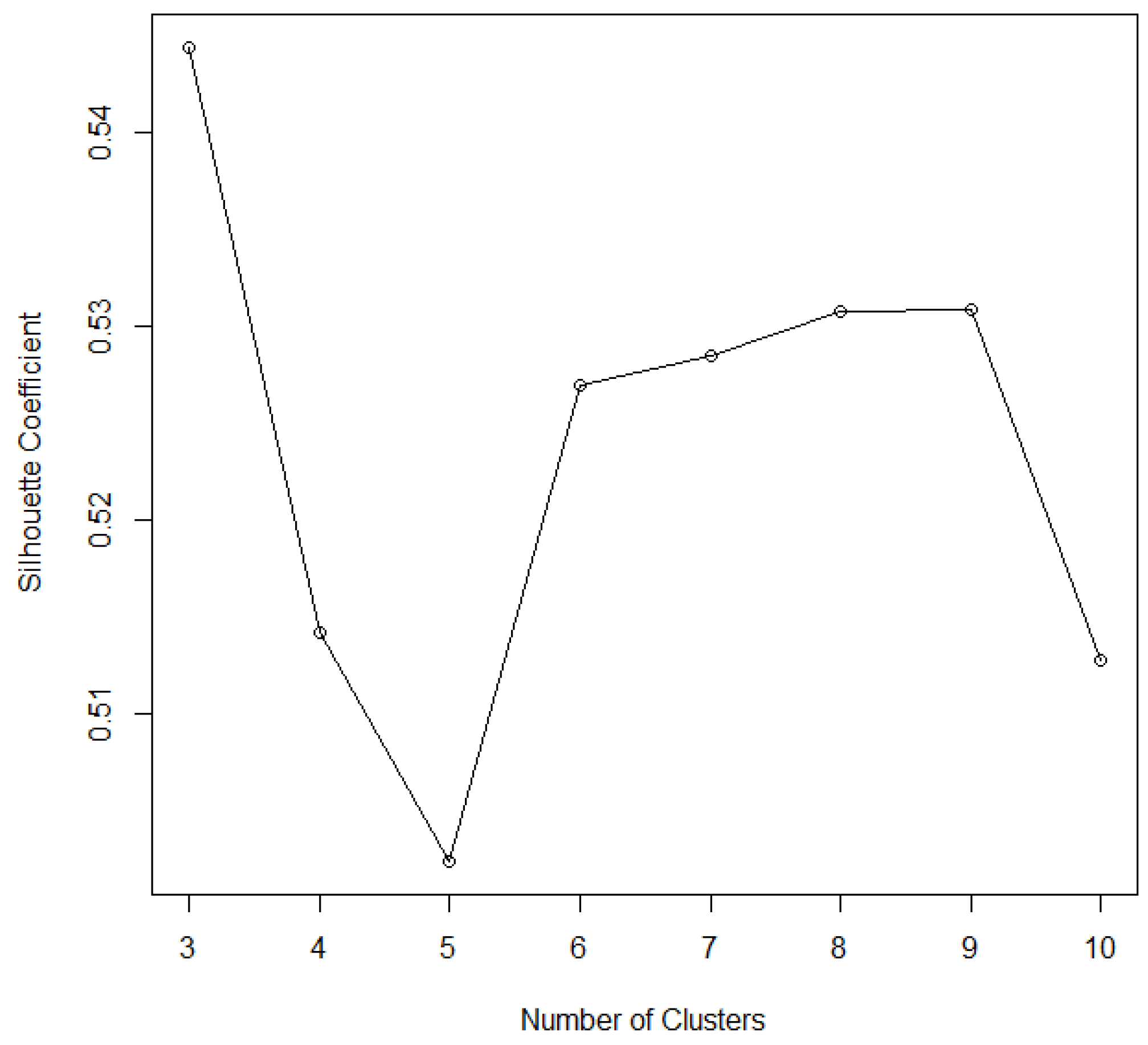
We calculate the SC of the away teams’ score when k ranges from 3 to 10 (two clusters are not enough to obviously distinguish a lot of data). Figure 1 shows the relationship between the k value and SC by k-means clustering to discretize the away teams’ score, where there is haphazard change in the SC value of the away teams’ score as the number of clusters increases from 3 to 10 in the 2014–15 season. We note that when k is 3, SC is at a maximum with a value of 0.545. Thus, the cluster number of the away teams’ score is assumed to be 3.

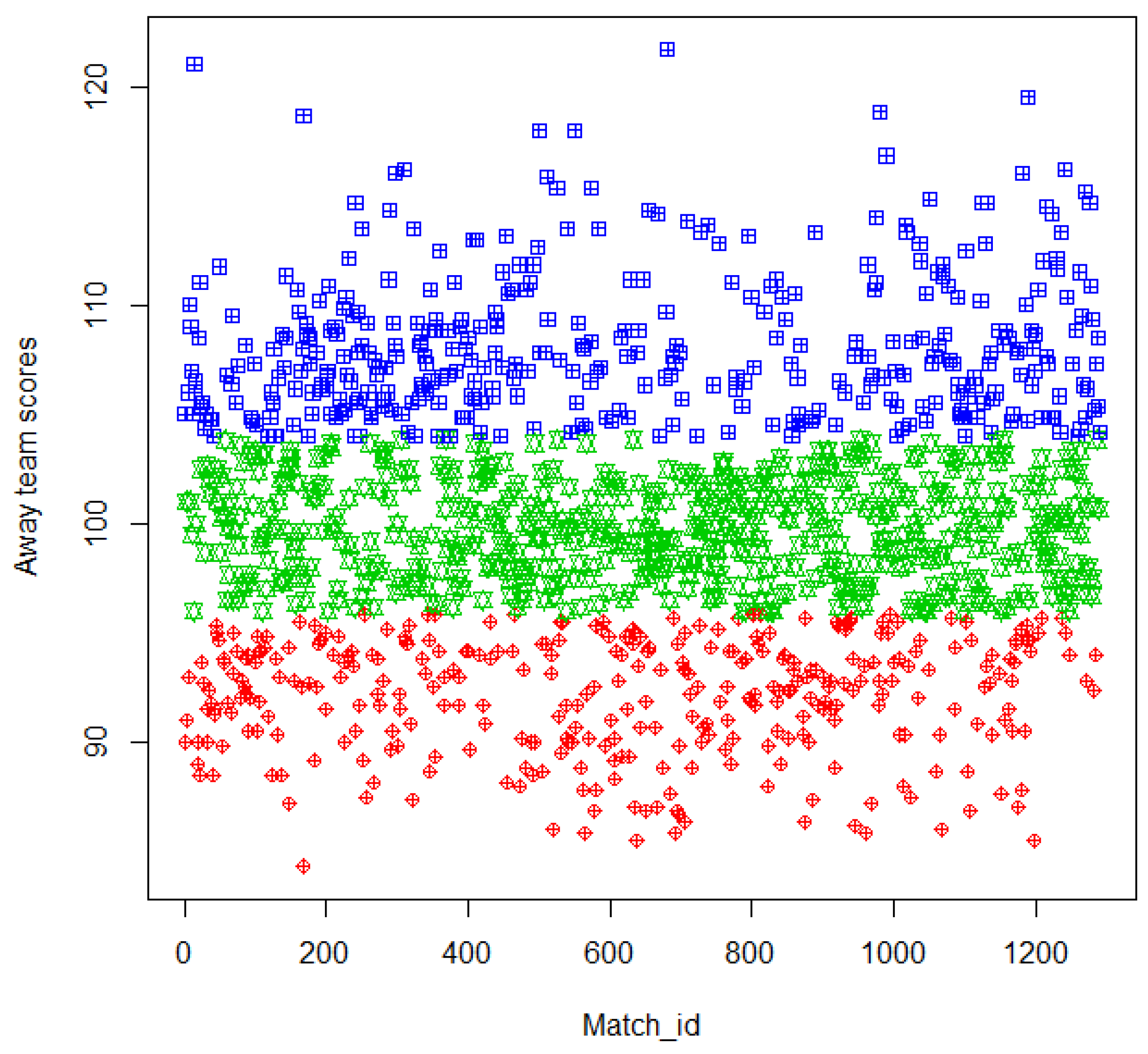
Figure 2 shows discrete values of the away teams’ score after k-means clustering when the SC is 0.545 and the distribution in each cluster is also indicated by different colors. The top blue cluster contains games whose away team scores range between 104 and 125. Ranges for the green (middle) and red (bottom) clusters are 97 to 103 and 80 to 96 respectively. We use k-means clustering to discretize home teams’ score values and other basic technical features for each game in the same way. Some samples of the experimental data set can be seen in the

Table 4. Discretized sample records of the experimental dataset.

Home Teams’ Features
$FG{M}_h$	$FG{A}_h$	$3P{M}_h$	$3P{A}_h$	$FT{M}_h$	$FT{A}_h$	$Ore{b}_h$	$Dre{b}_h$	$As{t}_h$	$St{l}_h$	$Bl{k}_h$	$T{O}_h$	$P{F}_h$	$PT{S}_h$
37.63	83.31	7.85	22.66	14.35	19.02	9.50	31.68	24.26	8.82	4.18	14.49	18.65	98.6
37.63	83.31	7.85	18.94	14.35	19.02	7.17	35.01	24.26	6.94	6.50	12.42	22.07	94.48
37.63	84.75	10.74	26.11	17.80	25.44	11.27	32.59	24.26	8.82	6.50	12.42	19.87	106.59
37.63	80.20	7.85	26.11	17.80	22.35	9.50	29.60	22.97	7.90	4.18	15.14	18.65	98.60
37.63	86.12	10.74	34.05	17.80	23.80	12.30	31.68	21.97	9.64	3.36	16.09	22.07	102.39
37.63	77.95	7.85	20.87	17.80	20.76	7.17	30.77	24.26	6.94	4.18	16.09	20.98	102.39
40.85	87.78	7.85	18.94	17.80	25.44	13.39	36.94	19.96	6.94	5.66	12.42	20.98	106.59
Away Teams’ Features															Home Team
$FG{M}_a$	$FG{A}_a$	$3P{M}_a$	$3P{A}_a$	$FT{M}_a$	$FT{A}_a$	$Ore{b}_a$	$Dre{b}_a$	$As{t}_a$	$St{l}_a$	$Bl{k}_a$	$T{O}_a$	$P{F}_a$	$PT{S}_a$		Win
40.36	82.6	7.77	18.40	20.61	26.54	10.34	32.16	22.40	6.59	4.08	16.19	21.65	108.43		1
36.76	73.84	7.77	21.63	16.85	24.42	8.26	28.68	19.34	9.00	3.76	13.17	21.65	100.06		1
37.73	86.81	5.39	18.40	16.85	20.34	12.48	28.68	21.66	7.76	5.15	12.42	20.45	100.06		1
38.88	79.5	10.49	21.63	15.58	20.34	7.59	32.16	24.13	7.76	5.71	17.36	22.79	100.06		0
35.66	85.13	7.77	21.63	17.90	24.42	10.83	35.50	19.34	7.18	5.71	11.74	19.09	100.06		1
37.73	85.13	5.39	18.40	16.85	20.34	11.48	32.16	20.70	7.18	5.15	12.42	16.32	100.06		1
42.48	86.81	10.49	24.73	16.85	22.41	12.48	32.16	20.70	8.40	5.71	12.42	19.09	108.43		1

.

Subscripts h and a in Table 4 indicate the home team and away team respectively, for example $FG{M}_h$ means Field Goal Made by the home team; the abbreviations are derived from Table 1. In Table 4, the first 14 columns represent the home teams’ basic technical feature values after k-means clustering discretization. The last column is the home teams’ actual wins or losses of the game. Others represent the away home teams’ basic technical feature values after k-means clustering discretization. It is also the final dataset that is applied to train the NBAME model and make predictions for the NBA playoffs. We sort them by the date, separate them by season, save the data for each season to a file, and then use data in each file to train and test the NBAME model repeatedly.

4.2. The Results of the NBAME Model for Predicting the NBA Playoffs

We used the feature vectors to construct the NBAME model with the Maximum Entropy principle and trained the parameter ${\lambda }_k$ with the GIS algorithm. Then, we applied 28 basic technical features of the coming game to the NBAME model and calculated the probability of the home team’s victory in the game, $p(y|x)$. Since $p(y|x)$ is a continuous value, the model makes a prediction based on a defined threshold: with a threshold of 0.5, it makes a prediction based on the conditions set in Equation (11) (meaning that if our model outputs a probability greater than or equal to 0.5, we decide that the home team wins, else we decide that the home team loses)

$$f_k(x,y)=\left\{\begin{array}{cc}1(win),\hfill & p(y|x)\ge 0.5,\hfill \\ 0(lose),\hfill & p(y|x)<0.5.\hfill \end{array}\right.$$

(11)

Finally, we compared the decision of our model to the true outcome of the game. If it was the same, then we said the prediction of the NBAME model was right, and we added 1 to the count of the correct prediction. Eventually, we would get the total number of predictions correctly, and we divided it by the number instances from the data set that we used to test it, which is our model’s forecast accuracy. Accuracy was used as performance measure, and it was calculated by the following formula:

$$\mathrm{Accuracy}=\frac{\mathrm{number}\mathrm{of}\mathrm{correct}\mathrm{predictions}}{\mathrm{number}\mathrm{of}\mathrm{predictions}}.$$

(12)

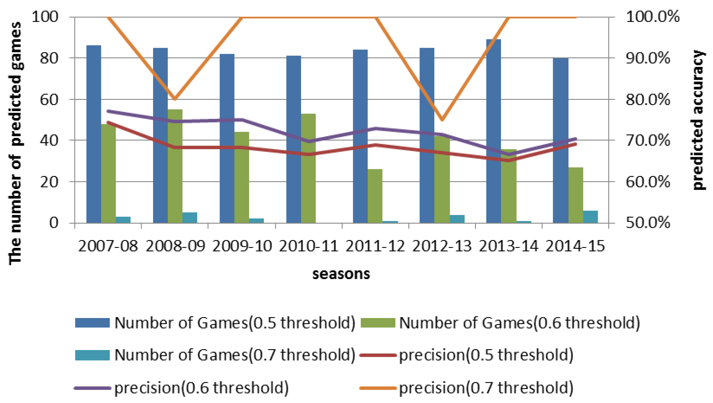
The NBAME model outputs the probability of the home team’s win in the upcoming game given the coming game’s features. The home team would be more likely to win if the model output a probability greater than the threshold value. At this point, it is important to note that setting a high confidence improves the accuracy of our model predictions with a drawback of predicting fewer games. For example, if we set a threshold of 0.6, it makes predictions based on conditions defined in Equation (13), implying that the model will not take a prediction decision for all games with output probabilities between 0.4 and 0.6:

$$f_k(x,y)=\left\{\begin{array}{cc}1(win),\hfill & p(y|x)\ge 0.6,\hfill \\ 0(lose),\hfill & p(y|x)\le 0.4.\hfill \end{array}\right.$$

(13)

Table 5. Prediction accuracy (in percentages) of the NBAME model with different thresholds.

Threshold	2007–08	2008–09	2009–10	2010–11	2011–12	2012–13	2013–14	2014–15
0.5	74.4	68.2	68.3	66.7	69.0	67.1	65.2	62.5
0.6	77.1	74.5	75.0	69.8	73.0	71.4	66.7	70.4
0.7	100.0	80.0	100.0	100.0	100.0	75.0	100.0	100.0

and

Table 6. The number of prediction games of the NBAME model with different thresholds.

Threshold	2007–08	2008–09	2009–10	2010–11	2011–12	2012–13	2013–14	2014–15
0.5	86	85	82	81	84	85	89	80
0.6	48	55	44	53	26	42	36	27
0.7	3	5	2	0	1	4	1	6

show the prediction results and the number of predicted games for each season using the defined thresholds of 0.5, 0.6, and 0.7.

From Table 5, the first row shows the prediction results for eight seasons of NBA playoff games by the NBAME model using a threshold of 0.5 (with a 0.5 threshold, the model makes predictions for all the playoffs). We notice that at 0.5 threshold, prediction accuracy of the model reaches as high as 74.4% in the 2007–08 season. If we increase the threshold, the number of games for which we could make a decision for all of the seasons reduces. For example, the number of predicted games decreased from 86 to 48 when we increased the threshold from 0.5 to 0.6 in the 2007–08 season; however, prediction accuracy improved from 74.4% to 77.1%. Similarly, when we increased the threshold from 0.6 to 0.7 in the 2007–08 season, the number of predicted games reduced from 48 to six with a 22.9% increase in prediction accuracy. This shows that we can trade the number of games for which we can make a prediction for an improved prediction accuracy, which can be of great commercial value. The results show that the proposed model is suitable to forecast the outcome of NBA playoffs while achieving high prediction accuracy.

Figure 3 shows the effect of varying thresholds on the number of predicted games and prediction accuracy for playoffs during the 2007–08 season and the 2014–15 season.

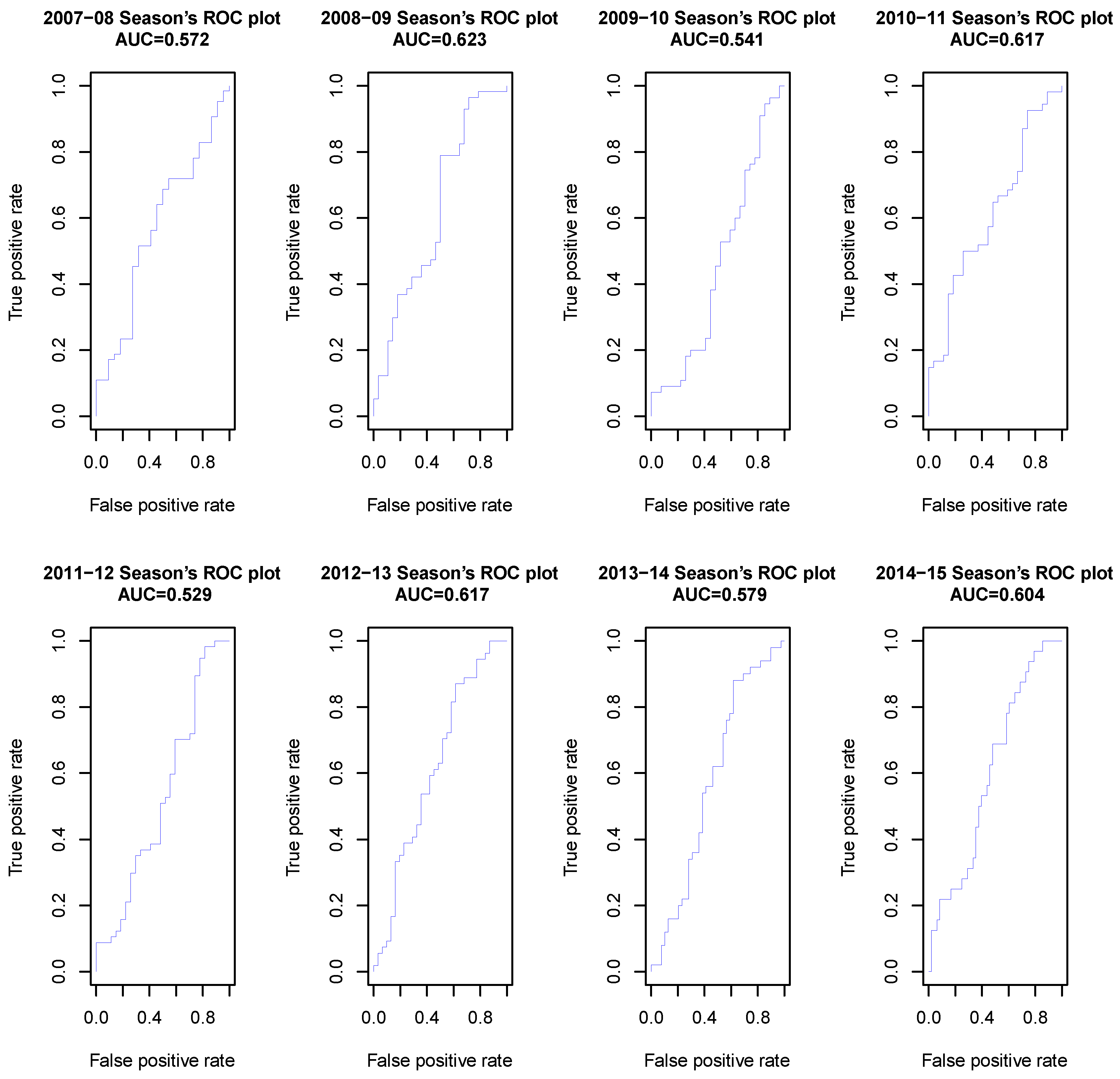
We also used Receiver Operating Characteristics (ROCs) [46,47] and the Area Under Curve (AUC) [48,49] to evaluate the quality of our NBAME model. We imported the probability of the home team’s winning and the true outcome of the game into R, and used prediction and performance function within the RROC package 1.0-7 [50] to plot the ROC curve and calculated AUC values for the eight seasons, and the results are presented in Figure 4.

4.3. Comparison of NBAME Model with Some Selected Existing Machine Learning Algorithms

To evaluate the NBAME model, we compared its performance with selected other machine learning algorithms (Naive Bayes, Logistic Regression, Back Propagation (BP) Neural Networks, Random Forest) in the Waikato Environment for Knowledge Analysis (WEKA 3.6) [51].

Table 7. Prediction accuracy (in percentages) of selected algorithms for NBA playoffs for seasons between 2007 and 2015.

Algorithm	2007–08	2008–09	2009–10	2010–11	2011–12	2012–13	2013–14	2014–15
Naive Bayes	54.7	61.5	56.1	59.3	53.6	58.8	59.3	55.0
Logistic Regression	61.6	57.1	61.0	61.7	60.7	64.7	62.6	60.0
BP Neural Networks	59.3	60.4	52.4	67.9	56.0	63.5	57.1	57.5
Random Forest	64.0	60.4	64.6	64.2	58.3	70.6	62.6	56.3
NBAME model	74.4	68.2	68.3	66.7	69.0	67.1	65.2	62.5

shows the results obtained when the features in Table 1 were used together with these algorithms to predict the outcome of NBA playoffs between 2007 and 2015 in Table 7, and Figure 5 presents a graphical representation of the results.

From Table 7 and Figure 5, we realize that our model outperformed all of the other classifiers for all seasons under consideration except for the 2010–11 season and the 2012–13 season, where our model was outperformed by Neural Networks and Random Forest, respectively. The Random Forest algorithm follows closely in the second position. The Naive Bayes had the lowest prediction accuracy with an average of about 60%, and this may have been caused by its assumption that all the features were independent, which was not the case. Accuracy results from the Neural Networks suffer adverse variations between seasons. For example, in the 2010–11 season, the Neural Networks registered impressive prediction accuracy at 67.9% but drastically reduced to 52.4% in the 2009–10 season. These variations could be explained by insufficiently small size of the training dataset that may have caused the model to overfit the data. Standard Logistic Regression, also a log-linear algorithm, had a relatively stable prediction accuracy for all seasons, similar to the NBAME. The NBAME outperformed the standard logistic regression because the former avoids overfitting by using regularisation techniques.

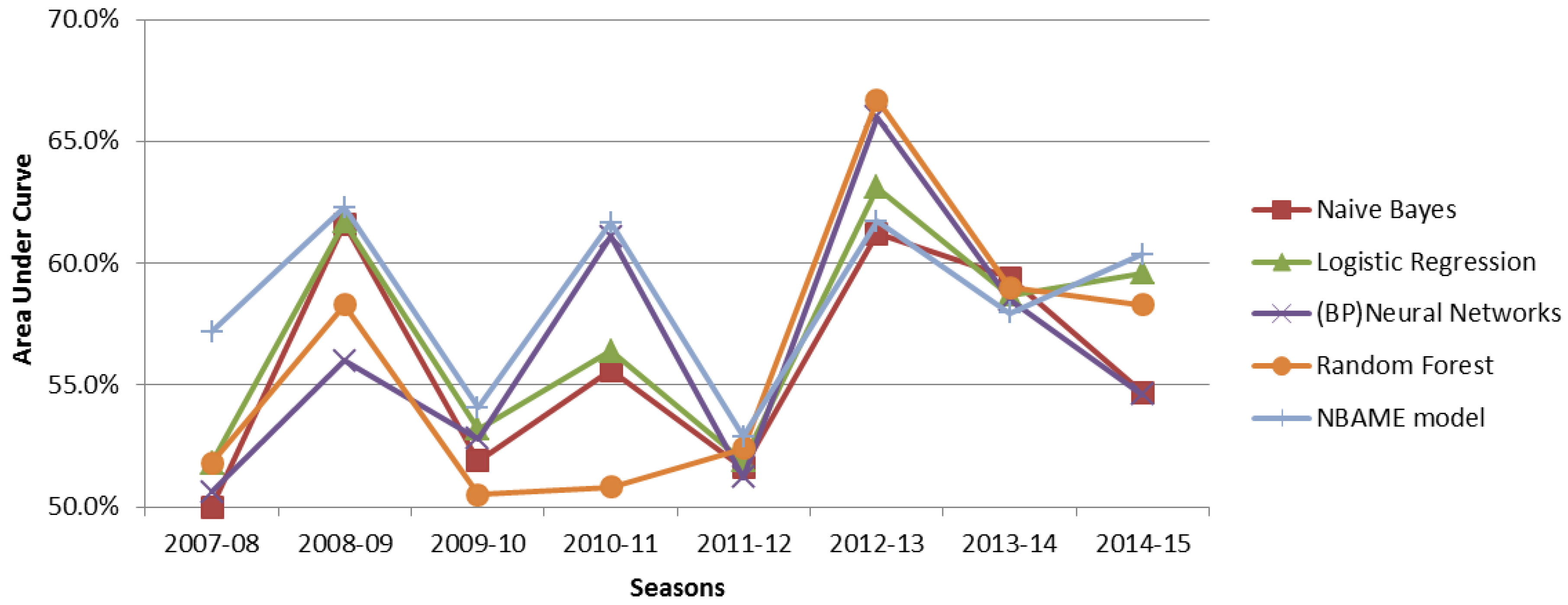
We give the AUC values in

Table 8. AUC (in percentages) values of selected algorithms for NBA playoffs for seasons between 2007 and 2015.

Algorithm	2007–08	2008–09	2009–10	2010–11	2011–12	2012–13	2013–14	2014–15
Naive Bayes	50.0	61.6	51.9	55.6	51.6	61.2	59.4	54.7
Logistic Regression	51.8	61.7	53.2	56.4	51.9	63.1	58.7	59.6
BP Neural Networks	50.6	56.0	52.8	61.1	51.2	66.0	58.5	54.6
Random Forest	51.8	58.3	50.5	50.8	52.4	66.7	59.0	58.3
NBAME model	57.2	62.3	54.1	61.7	52.9	61.7	57.9	60.4

, which make us view our NBAME model performance from another perspective, and Figure 5 shows a graphical representation of the same values.

Figure 6 shows that each algorithm’s AUC value is not very high due to a high number of features, yet working with only a small size of the training dataset [52]. The NBAME model is almost the top performing model in all seasons except 2012–13 and 2013–14. All algorithms show similar trends for all seasons. For example, they all performed very well in the 2012–13 season while experiencing the worst performance in the 2011–12 season. This indicates that some seasons are more difficult to predict than others. The difficulty in accurately forecasting results of a particular season is certainly triggered by unanticipated natural factors in the season; for example, the low performance in the 2011–12 season can be explained by the lockout that reduced the number of games from 82 to 66, thus reducing the training dataset size; in the same season, Derrick Rose, Joakim Noah, and David West were injured, leading to their failure to participate in the playoffs. Similarly, the controversy regarding Clippers’ owner Donald Sterling’s racist comments that arose in the 2013–14 season playoffs, and attracted protests from the Clippers and all NBA teams’ players, could have reduced the players’ morale, resulting in a very unpredictable season.

5. Conclusions

We applied the Maximum Entropy principle to construct the NBAME model and used the model to predict the outcome of the NBA playoffs from the 2007–08 season to the 2014–15 season. As seen in Section 4, the NBAME model is a good probability model for the prediction of NBA games. The prediction of NBA playoffs outcomes is a very difficult problem because there are many un-foreseeable factors such as the relative strengths of either team, the presence of injured players, players’ attitudes, and team managers’ operations that determine the winner or loser. Overall, the NBAME model is able to match or perform better than other machine learning algorithms.

The predictive model in this research was able to use the mean of each basic technical feature, respectively, from the most recent six games for both sides before the game started to accurately predict the outcome of the upcoming game. Possible extensions to this research would include exploring better methods to calculate the value of the features for the coming game, such as using more effective algorithms to preprocess the features of NBA dataset or looking for some comprehensive strengths as features.

References

1. Andrews, D. The (Trans) National Basketball Association: American Commodity-Sign Culture and Global-Local Conjuncturalism. In Articulating the Global and the Local: Globalization and Cultural Studies; Cvetovitch, A., Kellner, D., Eds.; Westview Press: Boulder, CO, USA, 1997; pp. 72–101. [Google Scholar]
2. Berri, D.J. National Basketball Association. In Handbook of Sports Economics Research; M.E. Sharpe: Armonk, NY, USA, 2006. [Google Scholar]
3. Zak, T.A.; Huang, C.J.; Siegfried, J.J. Production Efficiency: The Case of Professional Basketball. J. Bus. 1979, 52, 379–392. [Google Scholar] [CrossRef]
4. Harville, D.A. The Selection or Seeding of College Basketball or Football Teams for Postseason Competition. J. Am. Stat. Assoc. 2003, 98, 17–27. [Google Scholar] [CrossRef]
5. Bhandari, I.; Colet, E.; Parker, J.; Pines, Z.; Pratap, R.; Ramanujam, K. Advanced Scout: Data Mining and Knowledge Discovery in NBA Data. Data Min. Knowl. Discov. 1997, 1, 121–125. [Google Scholar] [CrossRef]
6. Loeffelholz, B.; Bednar, E.; Bauer, K.W. Predicting NBA games using neural networks. J. Quant. Anal. Sports 2009, 5, 1–15. [Google Scholar] [CrossRef]
7. Ivankovi, Z.; Rackovi, M.; Markoski, B.; Radosav, D.; Ivkovi, M. Analysis of basketball games using neural networks. In Proceedings of the 11th International Symposium on Computational Intelligence and Informatics (CINTI), Budapest, Hungary, 18–20 November 2010; pp. 251–256.
8. Beckler, M.; Wang, H.; Papamichael, M. NBA oracle. Zuletzt Besucht Am. 2013, 17, 2008–2009. [Google Scholar]
9. Delen, D.; Cogdell, D.; Kasap, N. A comparative analysis of data mining methods in predicting NCAA bowl outcomes. Int. J. Forecast. 2012, 28, 543–552. [Google Scholar] [CrossRef]
10. Miljković, D.; Gajić, L.; Kovačević, A.; Konjović, Z. The use of data mining for basketball matches outcomes prediction. In Proceedings of the 8th International Symposium on Intelligent Systems and Informatics (SISY), Subotica, Serbia, 10–11 September 2010; pp. 309–312.
11. Strumbelj, E.; Vracar, P. Simulating a basketball match with a homogeneous Markov model and forecasting the outcome. Int. J. Forecast. 2012, 28, 532–542. [Google Scholar] [CrossRef]
12. Vracar, P.; Strumbelj, E.; Kononenko, I. Modeling basketball play-by-play data. Expert Syst. Appl. 2016, 44, 58–66. [Google Scholar] [CrossRef]
13. Oh, M.; Keshri, S.; Iyengar, G. Graphical model for baskeball match simulation. In Proceddings of the 2015 MIT Sloan Sports Analytics Conference, Boston, MA, USA, 27–28 February 2015.
14. Stekler, H.O.; Sendor, D.; Verlander, R. Issues in sports forecasting. Int. J. Forecast. 2010, 26, 606–621. [Google Scholar] [CrossRef]
15. Haghighat, M.; Rastegari, H.; Nourafza, N. A Review of Data Mining Techniques for Result Prediction in Sports. Adv. Comput. Sci. 2013, 2, 7–12. [Google Scholar]
16. Shannon, C.E. A mathematical theory of communication. Bell Syst. Tech. J. 1948, 27, 379–423. [Google Scholar] [CrossRef]
17. Jaynes, E.T. Information theory and statistical mechanics. Phys. Rev. 1957, 106, 620–630. [Google Scholar] [CrossRef]
18. Leathwick, J.R.; Elith, J.; Francis, M.P.; Hastie, T.; Taylor, P. Variation in demersal fish species richness in the oceans surrounding New Zealand: an analysis using boosted regression trees. Mar. Ecol. Prog. Ser. 2006, 321, 267–281. [Google Scholar] [CrossRef]
19. Phillips, S.J.; Anderson, R.P.; Schapire, R.E. Maximum entropy modeling of species geographic distributions. Ecol. Model. 2006, 190, 231–259. [Google Scholar] [CrossRef]
20. Phillips, S.J.; Elith, J. On estimating probability of presence from use-availability or presence-background data. Ecology 2013, 94, 1409–1419. [Google Scholar] [CrossRef] [PubMed]
21. Berger, A.L.; Pietra, V.J.D.; Pietra, S.A.D. A maximum entropy approach to natural language processing. J. Comput. Linguist. 1996, 22, 39–71. [Google Scholar]
22. Yu, D.; Hinton, G.; Morgan, N.; Chien, J.-T.; Sagayama, S. Introduction to the special section on deep learning for speech and language processing. IEEE Trans. Audio Speech Lang. Process. 2012, 20, 4–6. [Google Scholar] [CrossRef]
23. Pham, A.-D.; Névéol, A.; Lavergne, T.; Yasunaga, D.; Clément, O.; Meyer, G.; Morello, R.; Burgun, A. Natural language processing of radiology reports for the detection of thromboembolic diseases and clinically relevant incidental findings. BMC Bioinform. 2014, 15, 266. [Google Scholar] [CrossRef] [PubMed]
24. Tseng, C.Y.; Tuszynski, J. Maximum Entropy in Drug Discovery. Entropy 2014, 16, 3754–3768. [Google Scholar] [CrossRef]
25. Xu, Y.; Wu, Z.; Jiang, L.; Song, X. A Maximum Entropy Method for a Robust Portfolio Problem. Entropy 2014, 16, 3401–3415. [Google Scholar] [CrossRef]
26. Phillips, S.J.; Dudik, M.; Schapire, R.E. A maximum entropy approach to species distribution modeling. In Proceedings of the Twenty-First International Conference on Machine learning, Banff, AB, Canada, 4–8 July 2004; p. 83.
27. Kotsiantis, S.; Kanellopoulos, D. Discretization techniques: A recent survey. GESTS Int. Trans. Comput. Sci. Eng. 2006, 32, 47–58. [Google Scholar]
28. Silva, J.A.; Faria, E.R.; Barros, R.C.; Hruschka, E.R.; de Carvalho André, C.P.L.F.; Gama, J. Data stream clustering: A survey. J. ACM Comput. Surv. 2013, 46, 13. [Google Scholar] [CrossRef]
29. Qu, J.; Zhang, J.; Huang, C.; Xie, B.; Wang, Y.; Zhang, X.-S. A novel discretization method for processing digital gene expression profiles. In Proceedings of the 7th International Conference on Systems Biology, Huangshan, China, 23–25 August 2013; pp. 134–138.
30. Jacques, J.; Preda, C. Functional data clustering: A survey. Adv. Data Anal. Classif. 2014, 8, 231–255. [Google Scholar] [CrossRef]
31. Garcia, S.; Luengo, J.; Herrera, F. Discretization. In Data Preprocessing in Data Mining; Springer: Cham, Switzerland, 2015; pp. 245–283. [Google Scholar]
32. Madhu, G.; Rajinikanth, T.V.; Govardhan, A. Improve the classifier accuracy for continuous attributes in biomedical datasets using a new discretization method. Procedia Comput. Sci. 2014, 31, 671–679. [Google Scholar] [CrossRef]
33. Kaya, F. Discretizing Continuous Features for Naive Bayes and C4.5 Classifiers. Available online: http://www.cs.umd.edu/sites/default/files/scholarly_papers/fatih-kaya_1.pdf (accessed on 5 December 2016).
34. Kerber, R. Chimerge: Discretization of numeric attributes. In Proceedings of the Tenth National Conference on Artificial intelligence, San Jose, CA, USA, 12–16 July 1992; pp. 123–128.
35. Monti, S.; Cooper, G.F. A latent variable model for multivariate discretization. In Proceedings of the Seventh International Workshop on Artificial Intelligence and Statistics, Fort Lauderdale, FL, USA, 4–6 January 1999.
36. Jain, A.K. Data Clustering: 50 Years Beyond K-Means. Pattern Recognit. Lett. 2010, 31, 651–666. [Google Scholar] [CrossRef]
37. Lloyd, S.P. Least Squares Quantization in PCM. IEEE Trans. Inf. Theory 1982, 28, 129–137. [Google Scholar] [CrossRef]
38. Tan, P.-N.; Steinbach, M.; Kumar, V. Introduction to Data Mining; Pearson: London, UK, 2005; p. 796. [Google Scholar]
39. Kumar, A.; Sinha, R.; Bhattacherjee, V.; Verma, D.S.; Singh, S. Modeling using K-means clustering algorithm. In Proceedings of the 1st International Conference on Recent Advances in Information Technology, Dhanbad, India, 15–17 March 2012; pp. 554–558.
40. Patankar, N.; Salkar, S. On the use of Side Information Based Improved K-Means Algorithm for Text Clustering. Int. J. Emerg. Trends Technol. 2015, 2, 369–374. [Google Scholar]
41. Garcia, M.L.L.; Garcia-Rodenas, R.; Gomez, A.G. K-means algorithms for functional data. Neurocomputing 2015, 151, 231–245. [Google Scholar] [CrossRef]
42. Kanungo, T.; Mount, D.M.; Netanyahu, N.S.; Piatko, C.D.; Silverman, R.; Wu, A.Y. An efficient k-means clustering algorithm: analysis and implementation. IEEE Trans. Pattern Anal. Mach. Intell. 2002, 24, 881–892. [Google Scholar] [CrossRef]
43. Darroch, J.N.; Ratcliff, D. Generalized Iterative Scaling for Log-Linear Models. Ann. Math. Stat. 1972, 43, 1470–1480. [Google Scholar] [CrossRef]
44. Cluster Analysis Extended Rousseeuw et al. Available online: http://astrostatistics.psu.edu/su07/R/html/cluster/html/00Index.html (accessed on 5 December 2016).
45. Kaufman, L.; Rousseeuw, P.J. Finding Groups in Data: An Introduction to Cluster Analysis; Wiley: Hoboken, NJ, USA, 1990. [Google Scholar]
46. Huang, J.; Ling, C.X. Using AUC and accuracy in evaluating learning algorithms. IEEE Trans. Knowl. Data Eng. 2005, 17, 299–310. [Google Scholar] [CrossRef]
47. Yousef, W.A. Assessing classifiers in terms of the partial area under the ROC curve. Comput. Stat. Data Anal. 2013, 64, 51–70. [Google Scholar] [CrossRef]
48. Ling, C.X.; Huang, J.; Zhang, H. AUC: A statistically consistent and more discriminating measure than accuracy. In Proceedings of the 18th International Joint Conference on Artificial Intelligence, Acapulco, Mexico, 9–15 August 2003; pp. 519–524.
49. Sing, T.; Sander, O.; Beerenwinkel, N.; Lengauer, T. Visualizing the Performance of Scoring Classifiers. Available online: https://rdrr.io/cran/ROCR/ (accessed on 5 December 2016).
50. Sing, T.; Sander, O.; Beerenwinkel, N.; Lengauer, T. Package ’ROCR’. Available online: https://cran.r-project.org/web/packages/ROCR/ROCR.pdf (accessed on 5 December 2016).
51. Hall, M.; Frank, E.; Holmes, G.; Pfahringer, B.; Reutemann, P.; Witten, I.H. The WEKA data mining software: An update. ACM SIGKDD Explor. Newsl. 2009, 11, 10–18. [Google Scholar] [CrossRef]
52. NBA Datasets 2007–15 Seasons. Available online: https://drive.google.com/open?id=0BwWkZ4LiPwITZjF3dk VNMVZ4SDg (accessed on 15 December 2016).
Figure 1. Silhouette Coefficient (SC) with the change of clusters.
Entropy 18 00450 g001
Figure 2. Three clusters for away teams’ scores.
Entropy 18 00450 g002
Figure 3. The number and accuracy of predictions with different confidence by the NBAME model from the 2007–08 season to the 2014–15 season playoffs.
Entropy 18 00450 g003
Figure 4. ROC curves and AUC values of prediction using the NBAME model from the 2007–08 season to the 2014–15 season playoffs.
Entropy 18 00450 g004
Figure 5. Comparison of the accuracy of the NBAME model against some machine learning algorithms.
Entropy 18 00450 g005
Figure 6. Comparison of AUC of the NBAME model against some machine learning algorithms.
Entropy 18 00450 g006