Grey Coupled Prediction Model for Traffic Flow with Panel Data Characteristics

Abstract

This paper studies the grey coupled prediction problem of traffic data with panel data characteristics. Traffic flow data collected continuously at the same site typically has panel data characteristics. The longitudinal data (daily flow) is time-series data, which show an obvious intra-day trend and can be predicted using the autoregressive integrated moving average (ARIMA) model. The cross-sectional data is composed of observations at the same time intervals on different days and shows weekly seasonality and limited data characteristics; this data can be predicted using the rolling seasonal grey model (RSDGM(1,1)). The length of the rolling sequence is determined using matrix perturbation analysis. Then, a coupled model is established based on the ARIMA and RSDGM(1,1) models; the coupled prediction is achieved at the intersection of the time-series data and cross-sectional data, and the weights are determined using grey relational analysis. Finally, numerical experiments on 16 groups of cross-sectional data show that the RSDGM(1,1) model has good adaptability and stability and can effectively predict changes in traffic flow. The performance of the coupled model is also better than that of the benchmark model, the coupled model with equal weights and the Bayesian combination model.

1. Introduction

Traffic flow prediction, particularly with regard to urbanization in China, has attracted the attention of scholars over the past 20 years. Traffic flow prediction is a key problem in the development of advanced traveler information systems (ATIS) and advanced traffic management systems (ATMS), which can provide accurate traffic information that can be used in traffic management signal system optimization. To address the complex characteristics of traffic flow, many theories are used for traffic flow prediction, from classical mathematical physics models to support vector machines (SVMs) and other evolutionary algorithms. New methods and techniques for improving the prediction accuracy are continuously presented [1,2]. Currently, many methods such as the regression method [3,4], time-series analysis [5,6], Kalman filter [7], grey model [8,9], spectral analysis [10,11], chaos theory [12], time-space model [13,14], neural network [15] and SVM [16,17] are widely used in traffic flow prediction.

Many studies have shown that urban traffic flow has a cyclical pattern, including intra-day trends and weekly trends [6,10,18]. The traffic flow series observed from the same site over several consecutive days shows an intra-day trend following an M-shaped curve. Kamarianakis et al. [3] used smooth-transition regressions to characterize the daily cycles of urban traffic flow. Chen et al. [19] analyzed the retrieval of intra-day trends for traffic flow series to address missing data and to improve traffic predictions. The weekly seasonality of traffic flow has been recognized and used by many scholars. Williams and Hoel [6] revealed the weekly seasonality of traffic flow and improved the traffic prediction using a 1-week lagged first seasonal difference. Tang et al. [20] proposed a hybrid prediction approach based on the weekly seasonality of traffic flow for different temporal scales, predicted future data using double exponential smoothing, and estimated the residual data using SVM. Zou et al. [21] considered the cyclical characteristics of freeway speed data by introducing a trigonometric regression function to capture the periodic component. Furthermore, the weekly cycle of traffic emissions revealed by Barmpadimos et al. [22] also reflect the weekly seasonality of traffic flow.

To excavate and utilize more information and to achieve better prediction, many studies have proposed the aggregation model to forecast short-term traffic flow. Zhang et al. [23] combined the seasonal autoregressive integrated moving average (SARIMA) and SVM models to predict traffic flow. Wang et al. [24] used the Bayesian combination method to integrate the results from autoregressive integrated moving average (ARIMA), Kalman filter and back propagation neural network predictions. Guo et al. [7] used the Kalman filter to calculate the real-time forecast of traffic flow under the seasonal autoregressive integrated moving average plus generalized autoregressive conditional heteroscedasticity (SARIMA + GARCH) structure. Zhang et al. [10] analyzed the intra-day trends, the deterministic part and the volatility components of traffic data and introduced spectral analysis techniques, ARIMA and GARCH models to predict these aspects of the data, respectively. Moreover, a hybrid empirical mode decomposition and autoregressive integrated moving average (EMD-ARIMA) approach was used to predict the short-term traffic speed on freeways [25]. However, most of the above models focus on the characteristics of nonlinearity, volatility and periodicity in a single time series but fail to take advantage of the characteristic information of more dimensions of traffic flow data, which may affect the prediction results.

Traffic flow data also have panel data characteristics outside of the one-dimensional time series [11]. Panel data for traffic flows can be thought of as multi-day traffic obtained over multiple time intervals for the same site. When recording traffic flow data, the data collected on the same day (e.g., 24 data points in 24 h) are time-series data, and the data that are collected at the same time interval (e.g., 7:00–8:00) are cross-sectional data. This data composes the H × D matrix pattern of data storage, referred to as panel data, where H is the number of time intervals in each day and D is the number of days in the historical data set. The ‘panel data’ presented here differs in meaning from the panel data used in economics, but the data are acquired and stored in the same way. The cross-sectional data is essentially considered to be a particular set of time-series data arranged in a horizontal direction. The cross-sectional data for the same time interval on multiple days show the weekly trends of the traffic flow, whereas the time-series data show the intra-day trends. Recently, based on these two traffic flow trends, Tan et al. [26] used the moving average (MA) model to predict intra-week trends and used the ARIMA model to predict intra-day trends; then, the two trends were aggregated by neural networks. Qiu [27] proposed a double cycle seasonal autoregressive integrated moving average model using two different ARIMA models to predict the intra-day trends and the weekly seasonality trend and then used an improved Bayesian algorithm to combine the models. All of the above models achieved good results. We found that constructing the model using the time-series data and the cross-sectional data of the traffic flow is an effective coupled forecasting method.

The studies of traffic flow with panel data characteristics have revealed an interesting finding: the cross-sectional data exhibits, in addition to the intra-week trend, a clear characteristic of limited data. All of the cross-sectional data, regardless of whether for 1 h flow or a shorter time interval flow, can only produce seven data points per week and only 28 data points within 4 weeks. Stale data loses its freshness and is no longer effective due to the interference of weather and other factors. We found that the grey system model was very suitable for tapping the inherent rules of this limited data. The grey prediction model has previously been successfully applied in the transportation field. Mao et al. [9] constructed a simple trigonometric grey GM(1,1) model for traffic flow forecasting. Guo et al. [8] established a delay and nonlinear grey model for urban road short-term traffic flow forecasting. Lu et al. [28] developed an optimized nonlinear grey Bernoulli model for traffic flow prediction. Yang and Liu [29] used grey numbers and grey sets to represent uncertainties in travel time. Bezuglov and Comert [30] established the GM(1,1) model and grey Verhulst model with Fourier error corrections for short-term traffic speed and travel time predictions. René S. et al. [31] developed an improved grey GM(1,4) model for German traffic safety predictions. Recently, a seasonal discrete grey model based on the cycle truncation accumulated generating operation (CTAGO) proposed by Xia [32] was successfully used in the seasonal forecasting of fashion retail. The model accurately captures the seasonal and limited data characteristics of fashion sales, which have a strong similarity to cross-sectional traffic flow data. The CTAGO can be used to address the intra-week trends of the cross-sectional traffic flow data. These studies show that the grey system theory has good performance for short-term traffic flow forecasting; however, it has not been used for prediction of traffic flow cross-sectional data with intra-week trends. Moreover, grey relational analysis, which is another active branch of grey system theory, has been successfully applied to management science and industrial control in practice [33,34]. Zhang et al. [35] used grey relational analysis for traffic congestion clustering judgment and obtained good results.

In summary, it is very meaningful to study the traffic flow prediction problem with panel data characteristics. Unlike the previous double time-series prediction, time-series data are predicted using the ARIMA model, and cross-sectional data are predicted using the proposed rolling seasonal grey forecasting model (RSDGM(1,1)) due to the characteristics of intra-week trends and limited data. Then, a coupled model is established to couple the time-series and cross-sectional data at the intersection, using the grey relational analysis to identify the weights. Finally, a case study is given.

The remaining parts of this paper are organized as follows: In Section 2, the fundamental theories of the grey prediction model are introduced, and a new RSDGM(1,1) based on the CTAGO is proposed. In Section 3, the RSDGM(1,1)-ARIMA coupled model is proposed, and grey relational analysis is used to identify the weights. In Section 4, numerical examples and experimental results are provided and discussed. Finally, in Section 5, some conclusions are provided based on the results.

2. Fundamental Theories

Grey system theory was founded by Deng Julong (1982) [36]. Since then, grey prediction theory and grey relational analysis have developed and matured rapidly; they have also been widely applied to analyses, models, predictions, decision making, and control of various systems. Grey system modeling finds the internal regularity of a given data series by accumulating operations. DGM(1,1), the discrete grey model with a first-order differential equation and one variable, has been shown to be equivalent to the GM(1,1) model under given conditions and to be simpler to use [37]. Xie and Liu discussed in detail the basic principles of DGM(1,1) [38], which has been widely used recently [32,39,40,41]. Here, we give a concise basic process of DGM(1,1).

2.1. DGM(1,1) Model

Assume that $x^{(0)}={(x^{(0)}(1),x^{(0)}(2),\cdots ,x^{(0)}(n))}^T$ is an original, non-negative sequence. The basic idea of the grey model is to find the internal regularity of a time series with limited data by accumulating operations. The most basic first-order accumulated generating operation (1-AGO) is defined as follows:

$$x^{(1)}(k)={\displaystyle \sum _{i=1}^k{x}^{(0)}(i)},k=1,2,\cdots n.$$

(1)

Its 1-AGO sequence is $x^{(1)}={(x^{(1)}(1),x^{(1)}(2),\cdots ,x^{(1)}(n))}^T$.

Then, the DGM(1,1) model [38] is:

$$x^{(1)}(k+1)={\beta }_1{x}^{(1)}(k)+{\beta }_2$$

(2)

Its parameter estimation is $\widehat{\beta }={[{\beta }_1,{\beta }_2]}^T={(B^{T}B)}^{-1}{B}^{T}Y$, where

$$Y=\left[\begin{array}{c}{x}^{(1)}(2)\\ x^{(1)}(3)\\ ⋮\\ x^{(1)}(n)\end{array}\right],B=\left[\begin{array}{cc}{x}^{(1)}(1)& 1\\ x^{(1)}(2)& 1\\ ⋮& ⋮\\ x^{(1)}(n-1)& 1\end{array}\right].$$

The solution (or time response function) of the DGM(1,1) model is given by:

$${\widehat{x}}^{(1)}(k+1)=(x^{(0)}(1)-\frac{{\beta }_2}{1-{\beta }_1}){\beta }_1^k+\frac{{\beta }_2}{1-{\beta }_1}$$

(3)

The restored values of $x^{(0)}(k)$ can be given by:

$${\widehat{x}}^{(0)}(k+1)=({\beta }_1-1)(x^{(0)}(1)-\frac{{\beta }_2}{1-{\beta }_1}){\beta }_1^{k-1}$$

(4)

2.2. The CTAGO Operator and Its Properties

When the original sequence is a seasonal sequence, the oscillation of the data causes the original sequence to be unable to effectively meet the smooth ratio of the grey modeling condition; thus, the prediction results appear to have a large deviation. Therefore, the CTAGO is introduced to obtain a better grey modeling smooth ratio condition.

Set q as the periodic value of the seasonal original raw sequence $x^{(0)}$; then, define the CTAGO [32] as follows:

$$y^{(0)}(k)=CTAGO(x^{(0)}(k))={\displaystyle \sum _{j=1}^q{x}^{(0)}(k+j-1)}\begin{array}{cc},& \forall k=1,2,\cdots n-q+1.\end{array}$$

(5)

If $r=n-q+1$, then $y^{(0)}={(y^{(0)}(1),y^{(0)}(2),\cdots ,y^{(0)}(r))}^T$ is denoted as the CTAGO sequence.

To investigate the relationship between the CTAGO sequence and the original sequence, we have the following:

$$y^{(0)}(k+1)-y^{(0)}(k)={\displaystyle \sum _{j=1}^q{x}^{(0)}(k+j)}-{\displaystyle \sum _{j=1}^q{x}^{(0)}(k+j-1)}=x^{(0)}(k+q)-x^{(0)}(k).$$

Thus,

$$y^{(0)}(k+1)-y^{(0)}(k)=x^{(0)}(k+q)-x^{(0)}(k)$$

(6)

Equation (6) shows that the difference information of the CTAGO sequence $y^{(0)}$ is equal to the cycle difference information of the corresponding data in the seasonal original data series, which is the basis of the GM(1,1) modeling data restored values.

On the other hand, given $\forall k=1,2,\cdots n-q+1$, if $x^{(0)}(k+q)>x^{(0)}(k)$, then $y^{(0)}(k+1)>y^{(0)}(k)$; if $x^{(0)}(k+q)<x^{(0)}(k)$, then $y^{(0)}(k+1)<y^{(0)}(k)$.

Combined with Equation (6) and the above analysis, if the original sequence has periodic oscillation, the CTAGO operator also has periodic oscillation. However, the CTAGO operator can weaken the oscillation of the original sequence, resulting in a relatively flat CTAGO sequence. Then, the CTAGO sequence can satisfy the smooth ratio of grey modeling in a given condition, which has the following properties:

Property 1.

Assume that $\forall k=1,2,\cdots ,n-q$, $q\ge 3$, $\overline{M}=\frac{1}{q+1}(x^{(0)}(k)+x^{(0)}(k+1)+\cdots +x^{(0)}(k+q))$, $M=\max \{x^{(0)}(k),\cdots ,x^{(0)}(k+q)\}$, and $m=\min \{x^{(0)}(k),\cdots ,x^{(0)}(k+q)\}$.

If $M<\frac{3}{2}\overline{M},m>\frac{1}{2}\overline{M}$ and the smooth ratios ${\rho }_y(k)=\frac{y^{(0)}(k)}{{\displaystyle \sum _{i=1}^{k-1}{y}^{(0)}(i)}}\in (\frac{1}{q-0.5},\frac{1}{2})$, then the smooth ratios satisfy the condition of the quasi-smooth sequence:

$$\frac{{\rho }_y(k+1)}{{\rho }_y(k)}<1,k=3,4,\cdots n-q-1,$$

The CTAGO sequence is a quasi-smooth sequence, which satisfies the conditions of DGM(1,1) grey modeling.

Proof. 

$\frac{{\rho }_y(k+1)}{{\rho }_y(k)}=\frac{y^{(0)}(k+1)}{{\displaystyle \sum _{i=1}^k{y}^{(0)}(i)}}/\frac{y^{(0)}(k)}{{\displaystyle \sum _{i=1}^{k-1}{y}^{(0)}(i)}}=\frac{y^{(0)}(k+1)}{y^{(0)}(k)}\cdot \frac{{\displaystyle \sum _{i=1}^{k-1}{y}^{(0)}(i)}}{{\displaystyle \sum _{i=1}^{k-1}{y}^{(0)}(i)+y^{(0)}(k)}}$

To prove $\frac{{\rho }_y(k+1)}{{\rho }_y(k)}<1$, that is, $y^{(0)}(k+1)\cdot {\displaystyle \sum _{i=1}^{k-1}{y}^{(0)}(i)}<y^{(0)}(k)({\displaystyle \sum _{i=1}^{k-1}{y}^{(0)}(i)+y^{(0)}(k)})$, we need to prove $\frac{y^{(0)}(k+1)-y^{(0)}(k)}{y^{(0)}(k)}<\frac{y^{(0)}(k)}{{\displaystyle \sum _{i=1}^{k-1}{y}^{(0)}(i)}}={\rho }_y(k)$

According to Equation (6), $\frac{y^{(0)}(k+1)-y^{(0)}(k)}{y^{(0)}(k)}=\frac{x^{(0)}(k+q)-x^{(0)}(k)}{x^{(0)}(k)+\cdots +x^{(0)}(k+q-1)}$

If $x^{(0)}(k+q)-x^{(0)}(k)<0$, the conclusion is clearly established; if $x^{(0)}(k+q)-x^{(0)}(k)>0$, by $M<\frac{3}{2}\overline{M},m>\frac{1}{2}\overline{M}$, $\frac{y^{(0)}(k+1)-y^{(0)}(k)}{y^{(0)}(k)}=\frac{x^{(0)}(k+q)-x^{(0)}(k)}{(q+1)\overline{M}-x^{(0)}(k+q)}<\frac{M-m}{(q+1)\overline{M}-M}<\frac{1.5\overline{M}-0.5\overline{M}}{(q+1)\overline{M}-1.5\overline{M}}=\frac{1}{q-0.5}$

Because the smooth ratios of the CTAGO sequence ${\rho }_y(k)\in (\frac{1}{q-0.5},\frac{1}{2})$,

$$\frac{y^{(0)}(k+1)-y^{(0)}(k)}{y^{(0)}(k)}<\frac{y^{(0)}(k)}{{\displaystyle \sum _{i=1}^{k-1}{y}^{(0)}(i)}}={\rho }_y(k)$$

Under the given conditions of property 1, the traffic flow cross-sectional data cycle is $q=7$, and the fluctuation range of the data is $m>\frac{1}{2}\overline{M},M<\frac{3}{2}\overline{M}$. When the smooth ratios of the CTAGO sequence are ${\rho }_y(k)\in (\frac{1}{6.5},\frac{1}{2})=(0.1538,0.5)$, the CTAGO sequence is a quasi-smooth sequence, which satisfies the conditions of DGM(1,1) grey modeling. However, the original cross-sectional data series does not satisfy the conditions of a quasi-smooth series, which is verified in the numerical experiment.

2.3. The DGM(1,1) Model of the CTAGO Operation

For CTAGO sequence $y^{(0)}={(y^{(0)}(1),y^{(0)}(2),\cdots ,y^{(0)}(r))}^T$, we can obtain its 1-AGO sequence $y^{(1)}={(y^{(1)}(1),y^{(1)}(2),\cdots ,y^{(1)}(r))}^T$, where

$$y^{(1)}(k)={\displaystyle \sum _{i=1}^k{y}^{(0)}(i)},k=1,2,\cdots ,r$$

(7)

Based on Equations (5) and (7), we can obtain:

$$y^{(1)}(k)={\displaystyle \sum _{i=1}^k{y}^{(0)}(i)}={\displaystyle \sum _{i=1}^k{\displaystyle \sum _{j=1}^q{x}^{(0)}(i+j-1)}},k=1,2,\cdots ,r$$

(8)

If we mark $A={\left(\begin{array}{ccccc}1& 0& 0& \cdots & 0\\ 1& 1& 0& \cdots & 0\\ 1& 1& 1& \cdots & 0\\ ⋮& ⋮& ⋮& & ⋮\\ 1& 1& 1& \cdots & 1\end{array}\right)}_r$ and $G={\left(\begin{array}{cccccccccc}1& 1& \cdots & 1& 0& \cdots & 0& 0& \cdots & 0\\ 0& 1& 1& \cdots & 1& \cdots & 0& 0& \cdots & 0\\ ⋮& ⋮& ⋮& ⋮& ⋮& & ⋮& ⋮& ⋮& ⋮\\ 0& 0& 0& 0& 0& \cdots & 1& 1& \cdots & 1\end{array}\right)}_{r\times n}$, the corresponding matrix expressions can be obtained as $y^{(0)}=G{x}^{(0)}$ and $y^{(1)}=A{y}^{(0)}=AG{x}^{(0)}$.

For the CTAGO sequence $y^{(0)}$, its DGM(1,1) model can be given by

$$y^{(1)}(k+1)={\beta }_1{y}^{(1)}(k)+{\beta }_2$$

(9)

The parameter identification has the following theorems:

Theorem 1.

If $P={({\beta }_1,{\beta }_2)}^T$, $Y={\left(\begin{array}{c}{y}^{(1)}(2)\\ y^{(1)}(3)\\ ⋮\\ y^{(1)}(r)\end{array}\right)}_{r-1}$, $B={\left(\begin{array}{cc}{y}^{(1)}(1)& 1\\ y^{(1)}(2)& 1\\ ⋮& ⋮\\ y^{(1)}(r-1)& 1\end{array}\right)}_{(r-1)\times 2}$, and the DGM(1,1) model parameter identification of the CTAGO sequence $y^{(0)}$ is

$$P={(B^{T}B)}^{-1}{B}^{T}Y={({(A_2{G}_{2}M)}^T{A}_2{G}_{2}M)}^{-1}{(A_2{G}_{2}M)}^T{A}_{1}GX,$$

where

$$\begin{gathered} B={\left(\begin{array}{cccc}1& 0& \cdots & 0\\ 1& 1& \cdots & 0\\ ⋮& ⋮& \ddots & ⋮\\ 1& 1& \cdots & 1\end{array}\right)}_{r-1}{\left(\begin{array}{cccccccccc}1& 1& \cdots & 1& 0& \cdots & 0& 0& \cdots & 0\\ 0& 1& \cdots & 1& 1& \cdots & 0& 0& \cdots & 0\\ ⋮& ⋮& ⋮& ⋮& ⋮& & ⋮& ⋮& ⋮& ⋮\\ 0& 0& 0& 0& 0& \cdots & 1& 1& \cdots & 1\end{array}\right)}_{(r-1)\times (n-1)}\cdot \left(\begin{array}{cc}{x}^{(0)}(1)& 1\\ x^{(0)}(2)& 0\\ ⋮& ⋮\\ x^{(0)}(n-1)& 0\end{array}\right)\triangleq A_2\cdot G_2\cdot M, \\ Y={\left(\begin{array}{ccccc}1& 1& 0& \cdots & 0\\ 1& 1& 1& \cdots & 0\\ ⋮& ⋮& ⋮& & ⋮\\ 1& 1& 1& \cdots & 1\end{array}\right)}_{(r-1)\times r}\cdot {\left(\begin{array}{cccccccccc}1& 1& \cdots & 1& 0& \cdots & 0& 0& \cdots & 0\\ 0& 1& 1& \cdots & 1& \cdots & 0& 0& \cdots & 0\\ ⋮& ⋮& ⋮& ⋮& ⋮& & ⋮& ⋮& ⋮& ⋮\\ 0& 0& 0& 0& 0& \cdots & 1& 1& \cdots & 1\end{array}\right)}_{r\times n}\cdot \left(\begin{array}{c}{x}^{(0)}(1)\\ x^{(0)}(2)\\ ⋮\\ x^{(0)}(n)\end{array}\right)\triangleq A_1\cdot G\cdot X. \end{gathered}$$

Proof. 

Based on $y^{(1)}(k+1)={\beta }_1{y}^{(1)}(k)+{\beta }_2$, $k=1,2,\cdots ,r-1$, we have $Y=BP$, that is,

$${\left[\begin{array}{c}{y}^{(1)}(2)\\ y^{(1)}(3)\\ ⋮\\ y^{(1)}(r)\end{array}\right]}_{r-1}={\left[\begin{array}{cc}{y}^{(1)}(1)& 1\\ y^{(1)}(2)& 1\\ ⋮& ⋮\\ y^{(1)}(r-1)& 1\end{array}\right]}_{(r-1)\times 2}\cdot \left(\begin{array}{c}{\beta }_1\\ {\beta }_2\end{array}\right),$$

by

$$Y={\left(\begin{array}{c}{y}^{(1)}(2)\\ y^{(1)}(3)\\ ⋮\\ y^{(1)}(r)\end{array}\right)}_{r-1}={\left(\begin{array}{ccccc}1& 1& 0& \cdots & 0\\ 1& 1& 1& \cdots & 0\\ ⋮& ⋮& ⋮& & ⋮\\ 1& 1& 1& \cdots & 1\end{array}\right)}_{(r-1)\times r}\cdot {\left(\begin{array}{c}{y}^{(0)}(1)\\ y^{(0)}(2)\\ ⋮\\ y^{(0)}(r)\end{array}\right)}_r={\left(\begin{array}{ccccc}1& 1& 0& \cdots & 0\\ 1& 1& 1& \cdots & 0\\ ⋮& ⋮& ⋮& & ⋮\\ 1& 1& 1& \cdots & 1\end{array}\right)}_{(r-1)\times r}\cdot {\left(\begin{array}{cccccccccc}1& 1& \cdots & 1& 0& \cdots & 0& 0& \cdots & 0\\ 0& 1& 1& \cdots & 1& \cdots & 0& 0& \cdots & 0\\ ⋮& ⋮& ⋮& ⋮& ⋮& & ⋮& ⋮& ⋮& ⋮\\ 0& 0& 0& 0& 0& \cdots & 1& 1& \cdots & 1\end{array}\right)}_{r\times n}\cdot \left(\begin{array}{c}{x}^{(0)}(1)\\ x^{(0)}(2)\\ ⋮\\ x^{(0)}(n)\end{array}\right)=A_1\cdot G\cdot X,$$

and

$$B={\left(\begin{array}{cc}{y}^{(1)}(1)& 1\\ y^{(1)}(2)& 1\\ ⋮& ⋮\\ y^{(1)}(r-1)& 1\end{array}\right)}_{(r-1)\times 2}={\left(\begin{array}{cccc}1& 0& \cdots & 0\\ 1& 1& \cdots & 0\\ ⋮& ⋮& \ddots & ⋮\\ 1& 1& \cdots & 1\end{array}\right)}_{r-1}{\left(\begin{array}{cc}{y}^{(0)}(1)& 1\\ y^{(0)}(2)& 0\\ ⋮& ⋮\\ y^{(0)}(r-1)& 0\end{array}\right)}_{(r-1)\times 2}={\left(\begin{array}{cccc}1& 0& \cdots & 0\\ 1& 1& \cdots & 0\\ ⋮& ⋮& \ddots & ⋮\\ 1& 1& \cdots & 1\end{array}\right)}_{r-1}{\left(\begin{array}{cccccccccc}1& 1& \cdots & 1& 0& \cdots & 0& 0& 0& 0\\ 0& 1& 1& \cdots & 1& \cdots & 0& 0& 0& 0\\ ⋮& ⋮& ⋮& ⋮& ⋮& & ⋮& ⋮& ⋮& ⋮\\ 0& 0& 0& 0& 0& \cdots & 1& 1& \cdots & 1\end{array}\right)}_{(r-1)\times (n-1)}\cdot \left(\begin{array}{cc}{x}^{(0)}(1)& 1\\ x^{(0)}(2)& 0\\ ⋮& ⋮\\ x^{(0)}(n-1)& 0\end{array}\right)=A_2\cdot G_2\cdot M$$

The matrix form of the DGM(1,1) model $Y=BP$ can be rewritten as

$$A_{1}GX=A_2{G}_{2}M\cdot P$$

Using the least squares method, the parameter solution is transformed into:

$$\min {\Vert A_{1}GX-A_2{G}_{2}M\cdot P\Vert }^2=\min {(A_{1}GX-A_2{G}_{2}M\cdot P)}^T(A_{1}GX-A_2{G}_{2}M\cdot P)$$

Using the derivation formula of the matrix, we have:

$$P=\left(\begin{array}{c}{\beta }_1\\ {\beta }_2\end{array}\right)={({(A_2{G}_{2}M)}^T{A}_2{G}_{2}M)}^{-1}{(A_2{G}_{2}M)}^T{A}_{1}GX.$$

Theorem 2.

If $B=A_2{G}_{2}M$, $Y=A_1\cdot G\cdot X$, and ${({\beta }_1,{\beta }_2)}^T={({(A_2{G}_{2}M)}^T{A}_2{G}_{2}M)}^{-1}{(A_2{G}_{2}M)}^T{A}_{1}GX$, then

(1)

The solution of the DGM(1,1) model (Equation (9)) is given by

$${\widehat{y}}^{(1)}(k+1)=(y^{(0)}(1)-\frac{{\beta }_2}{1-{\beta }_1}){\beta }_1^k+\frac{{\beta }_2}{1-{\beta }_1}$$

(10)

(2)

The time response function of the CTAGO sequence $y^{(0)}$ is given by

$${\widehat{y}}^{(0)}(k+1)=({\beta }_1-1)(y^{(0)}(1)-\frac{{\beta }_2}{1-{\beta }_1}){\beta }_1^{k-1}$$

(11)

(3)

After the inverse operation, the solution of the corresponding seasonal original sequence $x^{(0)}$ is given by

$${\widehat{x}}^{(0)}(k+1)=({\beta }_1-1)(y^{(0)}(1)-\frac{{\beta }_2}{1-{\beta }_1}){\beta }_1^{k-q}-y^{(0)}(k-q+1)+x^{(0)}(k-q+1),k=q,q+1,\cdots ,n$$

(12)

Proof. 

(1)

According to Equation (3), the following is clearly available:

(2)

${\widehat{y}}^{(0)}(k+1)$ $={\widehat{y}}^{(1)}(k+1)$ $-{\widehat{y}}^{(1)}(k)$ $=({\beta }_1-1)(y^{(0)}(1)-\frac{{\beta }_2}{1-{\beta }_1}){\beta }_1^{k-1}$, $k=1,2,\cdots ,n-1$.

(3)

Based on property 1 and Equation (11), we have

$$\begin{array}{l}{\widehat{x}}^{(0)}(k+1)={\widehat{y}}^{(0)}(k-q+2)-y^{(0)}(k-q+1)+x^{(0)}(k-q+1)\\ =({\beta }_1-1)(y^{(0)}(1)-\frac{{\beta }_2}{1-{\beta }_1}){\beta }_1^{k-q}-y^{(0)}(k-q+1)+x^{(0)}(k-q+1),k=q,q+1,\cdots ,n.\end{array}$$

In Theorem 2, based on the CTAGO and the 1-AGO transform, the grey DGM(1,1) model of the CTAGO sequence is established, which not only gives the solution of the CTAGO sequence but also gives the solution of the seasonal original sequence. Equation (12) is called the solution of the seasonal discrete grey forecasting model (SDGM(1,1)).

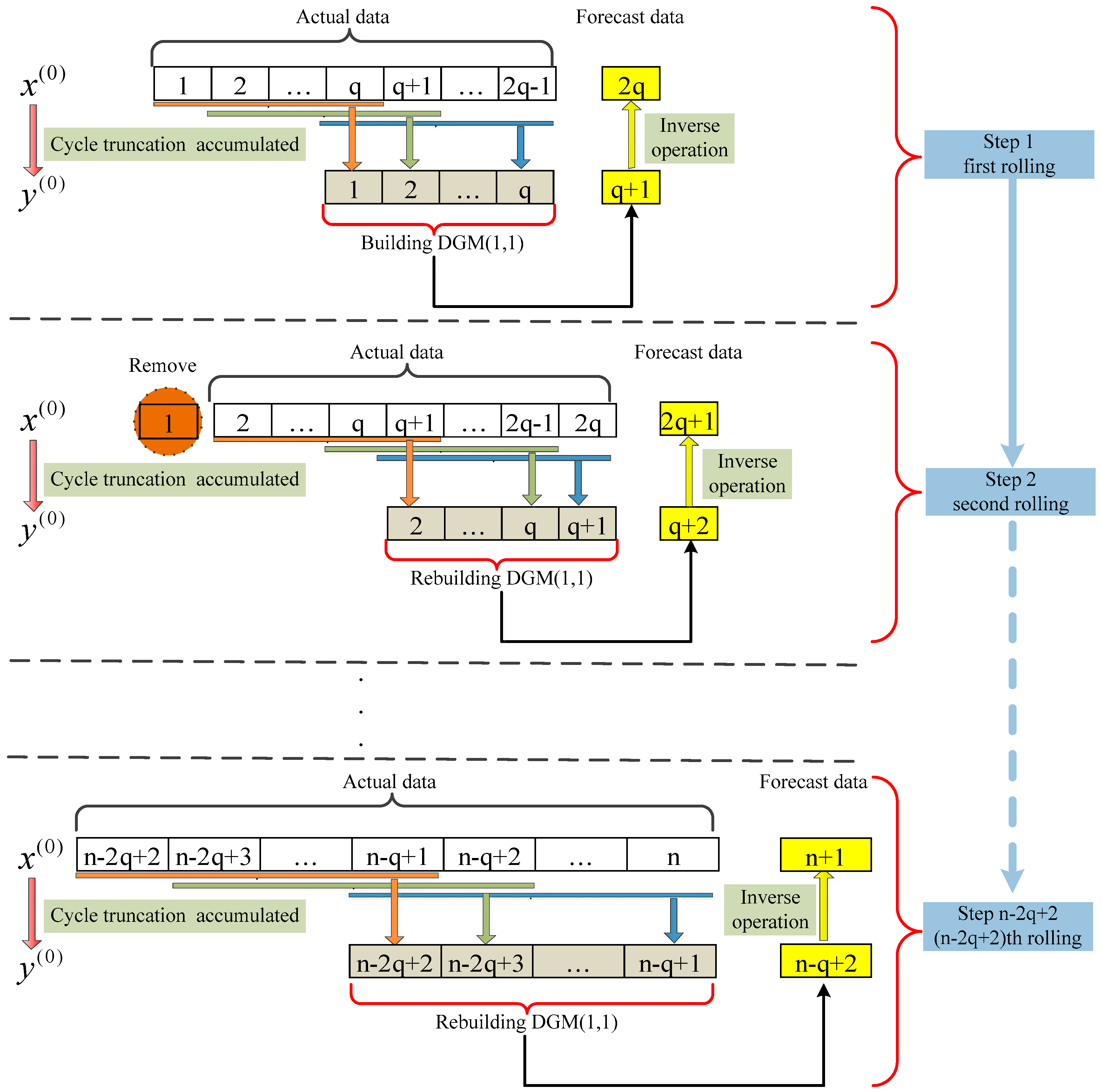
2.4. Rolling Grey Prediction Model: RDGM(1,1)

The rolling DGM(1,1) prediction model is a flexible extension of the DGM(1,1) model [42]. When the grey model is used to predict the traffic flow, the latest traffic information should be updated in real time, and the influence of the old information should be reduced step by step. Because the most recent data usually reflect the latest trends and characteristics of the object, in most cases, the rolling algorithm can improve the prediction accuracy [43]. Therefore, the rolling algorithm is used to keep the length of the data sequence unchanged, to constantly introduce new data, and to remove old data. The rolling DGM(1,1) process can be described as follows:

Step 1

The sequence $\{x^{(0)}(1),x^{(0)}(2),\cdots ,x^{(0)}(p)\}$ is first used for DGM(1,1) modeling, and ${\widehat{x}}^{(0)}(p+1)$ is predicted;

Step 2

The information is updated in real time, new observations $x^{(0)}(p+1)$ are introduced, and the old information $x^{(0)}(1)$ is removed. The rolling sequence $\{x^{(0)}(2),\cdots ,x^{(0)}(p),x^{(0)}(p+1)\}$ is used for DGM(1,1) modeling, and ${\widehat{x}}^{(0)}(p+2)$ is predicted;

Step 3

Step 2 is repeated until all the data points that need to be predicted have been obtained.

In the rolling DGM(1,1) prediction process, the length of the rolling data sequence is an important parameter. If this parameter is too small, it may cause prediction distortion due to lack of information. If the value is too large, it may cause data redundancy and will not be able to obtain the optimal effect. In the next section, we focus on the problem of the rolling sequence length in RSDGM(1,1).

2.5. Rolling Seasonal Grey Model of CTAGO Sequences: RSDGM(1,1)

The CTAGO sequence of the original seasonal data can improve the smooth ratio of the modeling sequence and expand the application range of the grey model. However, the DGM(1,1) model of the CTAGO sequence is still a small sample data model, which needs to be improved in the longer sequence. Wu [44,45,46] used matrix perturbation theory to explain the small sample data size of the grey prediction model.

The literature [46] shows that when $x^{(0)}(t)$ is disturbed, the disturbance boundary $L(x^{(0)}(t))$ of the parameter is an increasing function of $n$. Thus, when n increases, the parameter perturbation boundary increases, and the grey system model requires small sample modeling [46].

The rolling prediction model has better adaptability in practice and has been successfully applied in the fields of energy, electricity and financial forecasting [37,42,43,47]. For more elements of the seasonal traffic flow sequence, based on the idea of rolling metabolic prediction, the corresponding equal dimension rolling metabolism grey model is established, which is called the RSDGM(1,1) model. In the improved model, the key problem is determining the length of the rolling sequence so that it not only contains the seasonal information of the original sequence but also meets the small sample data modeling requirements of the grey model.

If the length of the seasonal original sequence data $x^{(0)}$ is n with a period of $q$, the length of its CTAGO sequence is $r=n-q+1$. Considering periodicity, we need $r=n-q+1\ge q$. To meet the new information priority principle, $r$ needs to be identified as the minimum value $q$; thus, $n=2q-1$.

The following theorem uses Lemma 1 to explain the weight preference of the corresponding time data of the previous period in the SDGM(1,1) model.

Lemma 1.

Suppose that x and x + h satisfy [46]

$${\Vert Bx-Y\Vert }_2=\min ,{\Vert (B+\mathrm{\Delta }B)x-(Y+\mathrm{\Delta }Y)\Vert }_2=\min ,$$

where $B,\mathrm{\Delta }B\in C^{m\times n}$ with $m\ge n$ and $Y\ne 0,\mathrm{\Delta }Y\in C^{m\times n}$.

Let $k_{+}={\Vert B^{†}\Vert }_2\Vert B\Vert ,$ ${\gamma }_{+}=1-{\Vert B^{†}\Vert }_2{\Vert \mathrm{\Delta }B\Vert }_2$, and $r_x=Y-Bx$, where $B^{†}$ is the pseudo-inverse of matrix $B$. If $rank(B)=rank(B+\mathrm{\Delta }B)=n$ and ${\Vert B^{†}\Vert }_2{\Vert \mathrm{\Delta }B\Vert }_2<1$, then

$$\Vert h\Vert \le \frac{k_{+}}{{\gamma }_{+}}\left(\frac{{\Vert \mathrm{\Delta }B\Vert }_2}{\Vert B\Vert }\Vert x\Vert +\frac{\Vert \mathrm{\Delta }Y\Vert }{\Vert B\Vert }+\frac{k_{+}}{{\gamma }_{+}}\frac{{\Vert \mathrm{\Delta }B\Vert }_2}{\Vert B\Vert }\frac{\Vert r_x\Vert }{\Vert B\Vert }\right)$$

Theorem 3.

Assume that the length of the seasonal original sequence $x^{(0)}$ is $n=2q-1$ and that the length of its CTAGO sequence $y^{(0)}$ is r = q. B and Y are the same as in Theorem 1. $L(x^{(0)}(t))$ is the perturbation bound when $\epsilon$ is regarded as a disturbance of $x^{(0)}(t)$ $(t=1,2,\cdots ,n-1,n)$. With Lemma 1, $rank(B)=rank(B+\mathrm{\Delta }B)=2$, ${\Vert B^{†}\Vert }_2{\Vert \mathrm{\Delta }B\Vert }_2<1$. If $\epsilon \ne 0$ and ${\Vert B^{†}\Vert }_2{\Vert \mathrm{\Delta }B\Vert }_2<1$, then

$$L(x^{(0)}(1))<L(x^{(0)}(2))<\cdots <L(x^{(0)}(q)),L(x^{(0)}(q))>L(x^{(0)}(q+1))>\cdots L(x^{(0)}(2q-1));$$

that is, $L(x^{(0)}(q))=\max \{L(x^{(0)}(1)),L(x^{(0)}(2)),\cdots ,L(x^{(0)}(2q-2)),L(x^{(0)}(2q-1))\}$.

Proof. 

(i)

If $\epsilon$ is regarded as a disturbance of $x^{(0)}(1)$, from Theorem 1,

$$\begin{array}{l}Y+\mathrm{\Delta }{Y}_1=A_1\cdot G\cdot \left(\begin{array}{c}{x}^{(0)}(1)+\epsilon \\ x^{(0)}(2)\\ ⋮\\ x^{(0)}(n)\end{array}\right)=Y+A_1\cdot G\cdot \left(\begin{array}{c}\epsilon \\ 0\\ ⋮\\ 0\end{array}\right),\mathrm{\Delta }{Y}_1=A_1\cdot G\cdot \left(\begin{array}{c}\epsilon \\ 0\\ ⋮\\ 0\end{array}\right)={\left(\begin{array}{c}\epsilon \\ \epsilon \\ ⋮\\ \epsilon \end{array}\right)}_{r-1},\\ B+\mathrm{\Delta }{B}_1=A_2\cdot G_2\cdot \left[\begin{array}{cc}{x}^{(0)}(1)+\epsilon & 1\\ x^{(0)}(2)& 0\\ ⋮& ⋮\\ x^{(0)}(n)& 0\end{array}\right]=B+A_2\cdot G_2\cdot \left[\begin{array}{cc}\epsilon & 0\\ 0& 0\\ ⋮& ⋮\\ 0& 0\end{array}\right],\\ \mathrm{\Delta }{B}_1=A_2\cdot G_2\cdot \left[\begin{array}{cc}\epsilon & 0\\ 0& 0\\ ⋮& ⋮\\ 0& 0\end{array}\right]={\left[\begin{array}{cc}\epsilon & 0\\ \epsilon & 0\\ ⋮& ⋮\\ \epsilon & 0\end{array}\right]}_{(r-1)\times 2},\mathrm{\Delta }{B}_1^T\cdot \mathrm{\Delta }{B}_1=\left(\begin{array}{cc}(r-1){\epsilon }^2& 0\\ 0& 0\end{array}\right),\end{array}$$

Therefore, ${\Vert \mathrm{\Delta }{B}_1\Vert }_2=\sqrt{{\lambda }_{\max }(\mathrm{\Delta }{B}_1^T\mathrm{\Delta }{B}_1)}=\sqrt{r-1}\left|\epsilon \right|=\sqrt{q-1}\left|\epsilon \right|,{\Vert \mathrm{\Delta }{Y}_1\Vert }_2=\sqrt{r-1}\left|\epsilon \right|=\sqrt{q-1}\left|\epsilon \right|$,

Thus,

$$L(x^{(0)}(1))=\frac{k_{+}}{{\gamma }_{+}}\left(\frac{{\Vert \mathrm{\Delta }B\Vert }_2}{\Vert B\Vert }\Vert x\Vert +\frac{\Vert \mathrm{\Delta }Y\Vert }{\Vert B\Vert }+\frac{k_{+}}{{\gamma }_{+}}\frac{{\Vert \mathrm{\Delta }B\Vert }_2}{\Vert B\Vert }\frac{\Vert r_x\Vert }{\Vert B\Vert }\right)=\frac{k_{+}}{{\gamma }_{+}}\left|\epsilon \right|\left(\frac{\sqrt{q-1}}{\Vert B\Vert }\Vert x\Vert +\frac{\sqrt{q-1}}{\Vert B\Vert }+\frac{k_{+}}{{\gamma }_{+}}\frac{\sqrt{q-1}}{\Vert B\Vert }\frac{\Vert r_x\Vert }{\Vert B\Vert }\right)$$

(13)

(ii)

If $\epsilon$ is regarded as a disturbance of $x^{(0)}(2)$,

$$\mathrm{\Delta }{Y}_2={\left(\begin{array}{c}2\epsilon \\ 2\epsilon \\ ⋮\\ 2\epsilon \end{array}\right)}_{r-1},\mathrm{\Delta }{B}_2={\left[\begin{array}{cc}\epsilon & 0\\ 2\epsilon & 0\\ ⋮& ⋮\\ 2\epsilon & 0\end{array}\right]}_{(r-1)\times 2},{\Vert \mathrm{\Delta }{B}_2\Vert }_2=\sqrt{4q-7}\left|\epsilon \right|,{\Vert \mathrm{\Delta }{Y}_2\Vert }_2=2\sqrt{q-1}\left|\epsilon \right|,$$

Similarly,

$$L(x^{(0)}(2))=\frac{k_{+}}{{\gamma }_{+}}\left|\epsilon \right|\left(\frac{\sqrt{4q-7}}{\Vert B\Vert }\Vert x\Vert +\frac{2\sqrt{q-1}}{\Vert B\Vert }+\frac{k_{+}}{{\gamma }_{+}}\frac{\sqrt{4q-7}}{\Vert B\Vert }\frac{\Vert r_x\Vert }{\Vert B\Vert }\right)$$

(14)

(iii)

If $\epsilon$ is regarded as a disturbance of $x^{(0)}(t)$ $(t=3,\cdots ,q-1,q)$, $\mathrm{\Delta }Y$ and $\mathrm{\Delta }B$ also change. Then,

$${\Vert \mathrm{\Delta }{B}_t\Vert }_2=\sqrt{{\displaystyle \sum _{j=1}^t{j}^2}+t^2(q-t-1)}\left|\epsilon \right|,{\Vert \mathrm{\Delta }{Y}_t\Vert }_2=\sqrt{{\displaystyle \sum _{j=2}^t{j}^2}+t^2(q-t)}\left|\epsilon \right|$$

When $t=3,\cdots ,q-1,q$,

$$L(x^{(0)}(t))=\frac{k_{+}}{{\gamma }_{+}}\left|\epsilon \right|\left(\frac{\sqrt{{\displaystyle \sum _{j=1}^t{j}^2}+t^2(q-t-1)}}{\Vert B\Vert }\Vert x\Vert +\frac{\sqrt{{\displaystyle \sum _{j=2}^t{j}^2}+t^2(q-t)}}{\Vert B\Vert }+\frac{k_{+}}{{\gamma }_{+}}\frac{\sqrt{{\displaystyle \sum _{j=1}^t{j}^2}+t^2(q-t-1)}}{\Vert B\Vert }\frac{\Vert r_x\Vert }{\Vert B\Vert }\right).$$

(15)

Set $f(t)={\displaystyle \sum _{j=2}^t{j}^2}+t^2(q-t)$, $g(t)={\displaystyle \sum _{j=1}^t{j}^2}+t^2(q-t-1)$.

If $2\le t\le q$ and $f(t)-f(t-1)=(2t-1)(q-t+1)>0$, then $g(t)-g(t-1)=(2t-1)(q-t)\ge 0$.

From Equations (13)–(16), we can obtain $L(x^{(0)}(1)<L(x^{(0)}(2)<\cdots <L(x^{(0)}(q))$.

(iv)

If $\epsilon$ is regarded as a disturbance of $x^{(0)}(t)$ $(t=q+1,q+2,\cdots ,2q-1,)$, $\mathrm{\Delta }Y$ and $\mathrm{\Delta }B$ also change; then,

$${\Vert \mathrm{\Delta }{B}_t\Vert }_2=\sqrt{{\displaystyle \sum _{j=1}^{n-t}{j}^2}}\left|\epsilon \right|(t=q+1,q+2,\cdots ,2q-2),{\Vert \mathrm{\Delta }{B}_{2q-1}\Vert }_2=0,{\Vert \mathrm{\Delta }{Y}_t\Vert }_2=\sqrt{{\displaystyle \sum _{j=1}^{n-t+1}{j}^2}}\left|\epsilon \right|;$$

thus,

$$L(x^{(0)}(t))=\frac{k_{+}}{{\gamma }_{+}}\left|\epsilon \right|\left(\frac{\sqrt{{\displaystyle \sum _{j=1}^{n-t}{j}^2}}}{\Vert B\Vert }\Vert x\Vert +\frac{\sqrt{{\displaystyle \sum _{j=1}^{n-t+1}{j}^2}}}{\Vert B\Vert }+\frac{k_{+}}{{\gamma }_{+}}\frac{\sqrt{{\displaystyle \sum _{j=1}^{n-t}{j}^2}}}{\Vert B\Vert }\frac{\Vert r_x\Vert }{\Vert B\Vert }\right),L(x^{(0)}(2q-1))=\frac{k_{+}}{{\gamma }_{+}}\frac{\left|\epsilon \right|}{\Vert B\Vert }$$

(16)

By contrasting Equations (15) and (16), we can obtain:

$$L(x^{(0)}(q))>L(x^{(0)}(q+1))>\cdots L(x^{(0)}(2q-1)).$$

In summary, $L(x^{(0)}(q))=\max \{L(x^{(0)}(1)),L(x^{(0)}(2)),\cdots ,L(x^{(0)}(2q-2)),L(x^{(0)}(2q-1))\}$.

Because ${\widehat{x}}^{(0)}(2q)$ $={\widehat{y}}^{(0)}(q+1)-y^{(0)}(q)+x^{(0)}(q)$, Theorem 3 shows that under the same perturbation situation, the parameter perturbation bound of $x^{(0)}(q)$ is the largest, which is the previous period of ${\widehat{x}}^{(0)}(2q)$ in the corresponding time data. Therefore, $x^{(0)}(q)$ has the greatest impact on the parameter estimates, which can be understood as the corresponding weight of the maximum. The equal dimension RSDGM(1,1) rolling model calls attention to the new information priority of the grey model and the periodic law of the original data.

When the sequence length of the RSDGM(1,1) model is determined, the prediction procedure of the RSDGM(1,1) is shown in Figure 1.

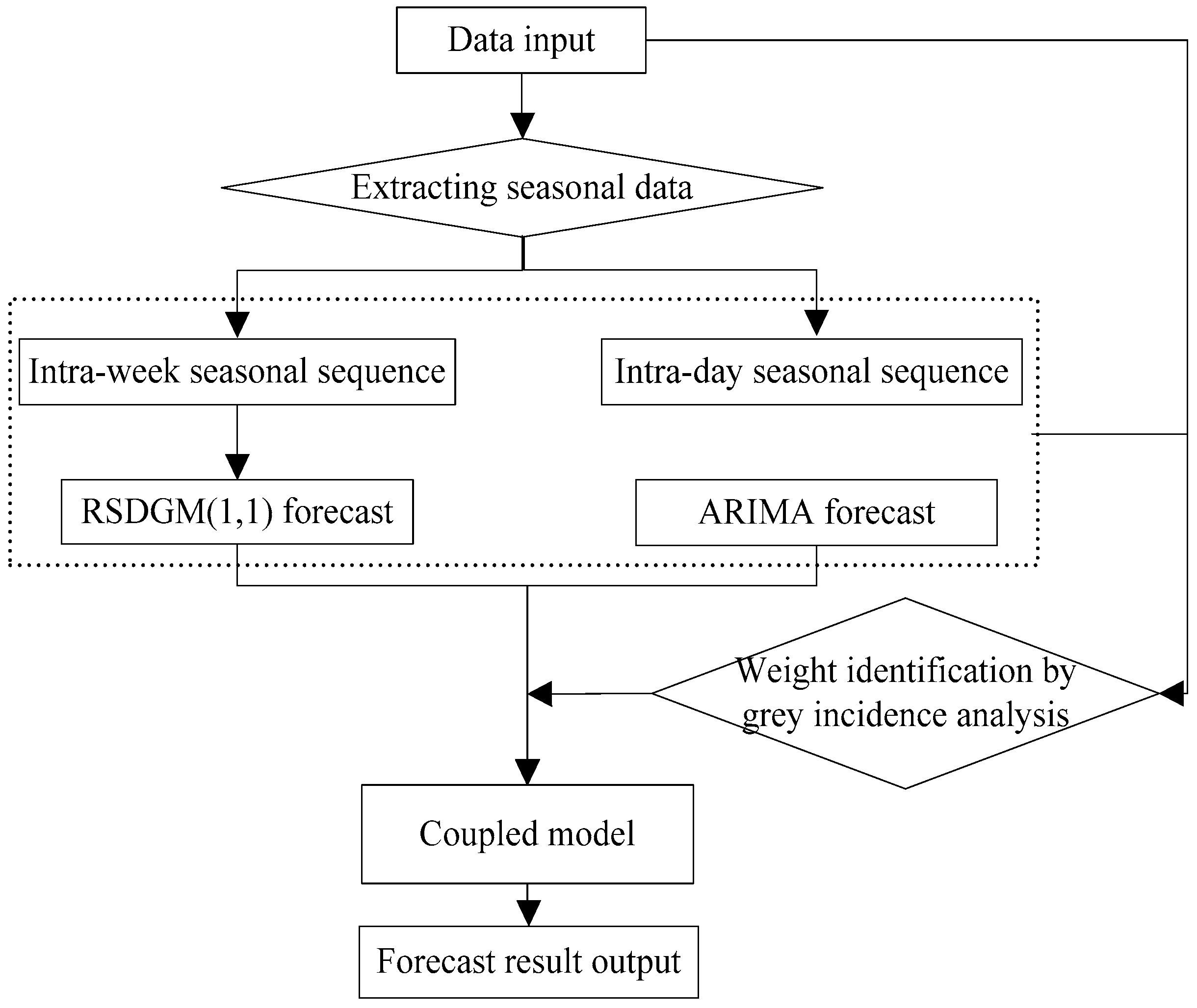
3. RSDGM(1,1)-ARIMA Coupled Model

For the time-series and cross-sectional traffic flow data, the intra-day trend of traffic flow for typical time-series data has been widely studied, and the ARIMA model is widely used in traffic flow time-series prediction. However, the proposed RSDGM(1,1) model is used to predict the cross-sectional data due to its typical characteristics of limited data and seasonal fluctuations. Then, a coupled model is established coupling the time-series and cross-sectional data at the intersection point, which is based on the nearness grey relational degree to identify the weights.

3.1. ARIMA Model

For the time-series traffic flow data, the ARIMA model is used to determine the regression-type relationship between the historical data and the future data, and a differencing technique is applied for the non-stationary data.

The time series $x_t$ that we want to study is always non-stationary; by proper differencing, we can obtain an ARIMA model [48] that is usually denoted as ARIMA ($p,d,q$):

$$\phi (B){(1-B)}^d{x}_t=C+\theta (B){\epsilon }_t$$

(17)

where $x_t$ is the traffic flow series and $B$ is the backshift operator $B^n{x}_t=x_{t-n}$;

$\phi (B)=1-{\phi }_{1}B-\cdots -{\phi }_P{B}^P$ is the autoregressive coefficient polynomial of the ARMA($p,q$) model;

$\theta (B)=1-{\theta }_{1}B-\cdots -{\theta }_q{B}^q$ is the moving smooth coefficient polynomial of the ARMA($p,q$) model;

$d$ is the frequency difference; $p$ is the lag order of AR; $q$ is the lag order of MA; $C$ is a constant; and $\left\{{\epsilon }_t\right\}$ is the zero mean white noise sequences.

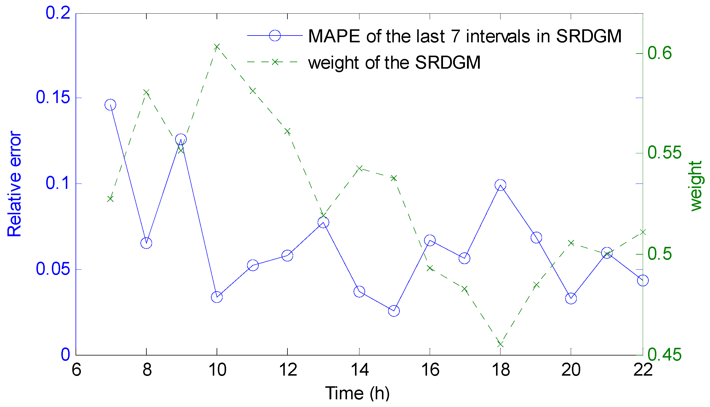
3.2. RSDGM(1,1)-ARIMA Coupled Model

The road traffic system is nonlinear, seasonal and uncertain; many single traffic flow models have advantages and disadvantages and corresponding applicable conditions and scope. Therefore, the comprehensive consideration of more factors and the use of a hybrid algorithm are important means of improving the effectiveness of traffic flow prediction.

In this paper, traffic flow panel data are collected; RSDGM(1,1) is used to predict the cross-sectional data that has weekly seasonal characteristics; and the ARIMA model is used to predict the time-series data. Then, at the intersection, the predictive values of the two models are coupled. At time $t+1$, the predictive value of the cross-sectional data is $Q_{t+1}^s$, its weight is $w_t^s$, the prediction value of the time-series data is $Q_{t+1}^a$, and there is a weighted value of $w_t^a$; thus, the time-series and cross-sectional data coupled prediction model is as follows:

$$Q_{t+1}=w_t^s{Q}_{t+1}^s+w_t^a{Q}_{t+1}^a$$

(18)

The coupled algorithm uses the nearness grey relational degree [33,34] to identify the weight.

The definition of the nearness grey relational degree is as follows:

Definition 1.

Assume that $X_i=(x_i(1),x_i(2),\cdots ,x_i(n))$ and $X_j=(x_j(1),x_j(2),\cdots ,x_j(n))$ [34].

Let $S_i-S_j={\displaystyle {\int }_1^n(X_i-X_j)}dt$; then,

$${\rho }_{ij}=\frac{1}{1+\left|S_i-S_j\right|}$$

(19)

is called the nearness grey relational degree of $X_i$ and $X_j$.

The single prediction model before time $t+1$ is used to predict the performance of the integrated $q$ phase, reflecting its weight in the coupled model. The higher the nearness grey relational degree is between the fitting value and the actual value of the single model, the greater the weight of the coupled model is; conversely, its weight is smaller.

The weights in a Bayesian combined model depend on the predictive performance of all the moments before time $t+1$; in other combination models, the weights are determined by only the prediction error of time t. In fact, according to the weekly seasonality of the cross-sectional data, taking the predictive nearness grey relational degree of the $q$ phase before the $t+1$ moment as a weight index can reflect the cycle information priority of the RSDGM(1,1) model, which is more in line with the actual needs. In the literature [24], time-series data take the predictive nearness grey relational degree of the q phase before $t+1$ as a weight index, and good results have been achieved with $q$ = 3, 5, or 7. In conclusion, in the coupled model, both cross-sectional data and time-series data will take the nearness grey relational degree in the $q$ = 7 phase before $t+1$ to identify the weights.

The coupled prediction model algorithm is as follows:

(1)

The fitting value and real value sequence of the 7 time intervals before $t+1$ are extracted from the RSDGM and ARIMA model prediction periods, respectively:

$$\begin{gathered} Q^s=(Q^s(t-q),Q^s(t-q+1),\cdots ,Q^s(t)),{\widehat{Q}}^s=({\widehat{Q}}^s(t-q),{\widehat{Q}}^s(t-q+1),\cdots ,{\widehat{Q}}^s(t)); \\ {Q}^a=(Q^a(t-q),Q^a(t-q+1),\cdots ,Q^a(t)),{\widehat{Q}}^a=({\widehat{Q}}^a(t-q),{\widehat{Q}}^a(t-q+1),\cdots ,{\widehat{Q}}^a(t)). \end{gathered}$$

(2)

According to Equation (19), the corresponding nearness grey relational degree ${\rho }_t^s$ and ${\rho }_t^a$ are obtained:

$${\rho }_t^s=\frac{1}{1+\left|Q^s-{\widehat{Q}}^s\right|},{\rho }_t^a=\frac{1}{1+\left|Q^a-{\widehat{Q}}^a\right|};$$

(3)

The corresponding weighted coefficients in the coupled model are determined by the nearness grey relational degree:

$$w_t^s={\rho }_t^s/({\rho }_t^s+{\rho }_t^a),w_t^a={\rho }_t^a/({\rho }_t^s+{\rho }_t^a);$$

(4)

Equation (18) is used to solve the time-series and cross-sectional data coupled prediction:

$$Q_{t+1}=w_t^s{Q}_{t+1}^s+w_t^a{Q}_{t+1}^a.$$

The coupled model forecasting process diagram is as follows in Figure 2.

4. Numerical Examples and Experimental Results

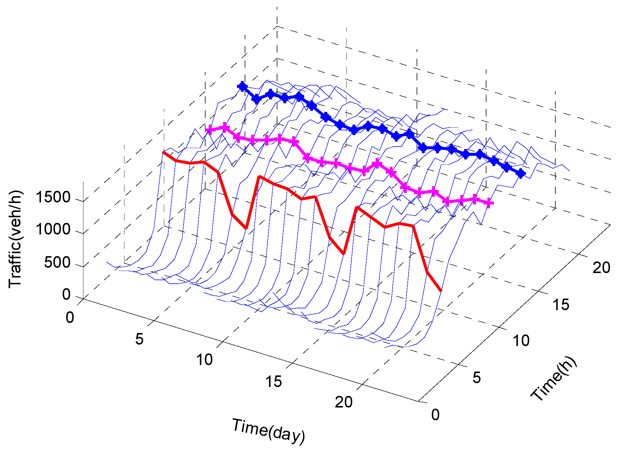
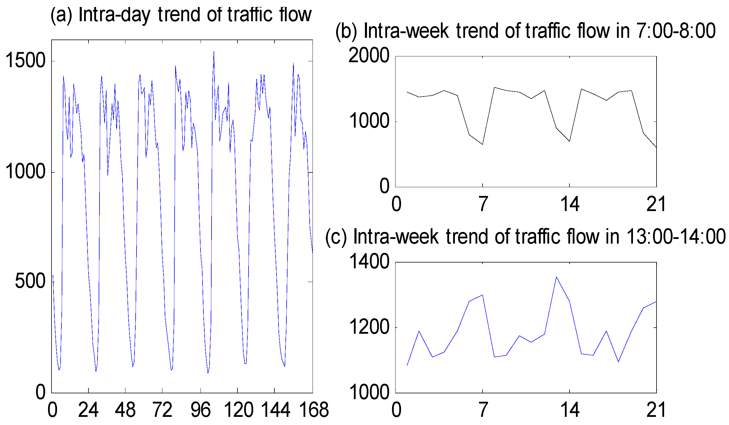
4.1. Data Description

The data used in the present study were measured on Shaoshan Road in Changsha, China. The selected road is one of the busy arterial roads in Changsha; it is an 8-lane road, with 4 lanes in each direction. The present study considered only the direction from south to north. At the intersection of Shaoshan Road and Jiefang Road, four loop detectors located on the straight lane were used to obtain the required traffic data. The traffic data was output by the SCATS Traffic Reporter system with a 5-min acquisition cycle [49]. Each detector collected 288 traffic data points per day. Flow data from 21 consecutive days (14 October to 3 November 2013) were collected from the loop detectors and used for model development. The traffic flow data corresponding to 4 November 2013, was used for model validation. For this study, we converted the raw data into hourly traffic flow with 24 data points per day. The 3D display of the panel data is shown in Figure 3. Figure 4 shows that because the weekend traffic flow trend differs significantly from that of the working day, the cross-sectional data have a significant weekly seasonality with a period of 7; the time-series data have obvious intra-day seasonal trends with a period of 24.

The model predictive performance evaluation used the absolute percentage error (APE) and the mean absolute percentage error (MAPE) to describe the degree of deviation of the traffic flow predictive value from the actual value. In addition, the equal coefficient (EC) was used to describe the degree of fit of the prediction curve to the measured curve. $x(k)$ are the measured values of traffic flow, $\widehat{x}(k)$ are the predicted values, and N is the number of data points. Then,

$$APE=\frac{\left|x(k)-\widehat{x}(k)\right|}{x(k)}\times 100\%$$

(20)

$$MAPE=\frac{1}{N}{\displaystyle \sum _{k=1}^N\frac{\left|\widehat{x}(k)-x(k)\right|}{x(k)}}\times 100\%$$

(21)

$$EC=1-\frac{\sqrt{{\displaystyle \sum {(\widehat{x}(k)-x(k))}^2}}}{\sqrt{{\displaystyle \sum {(x(k))}^2}}+\sqrt{{\displaystyle \sum {(\widehat{x}(k))}^2}}}$$

(22)

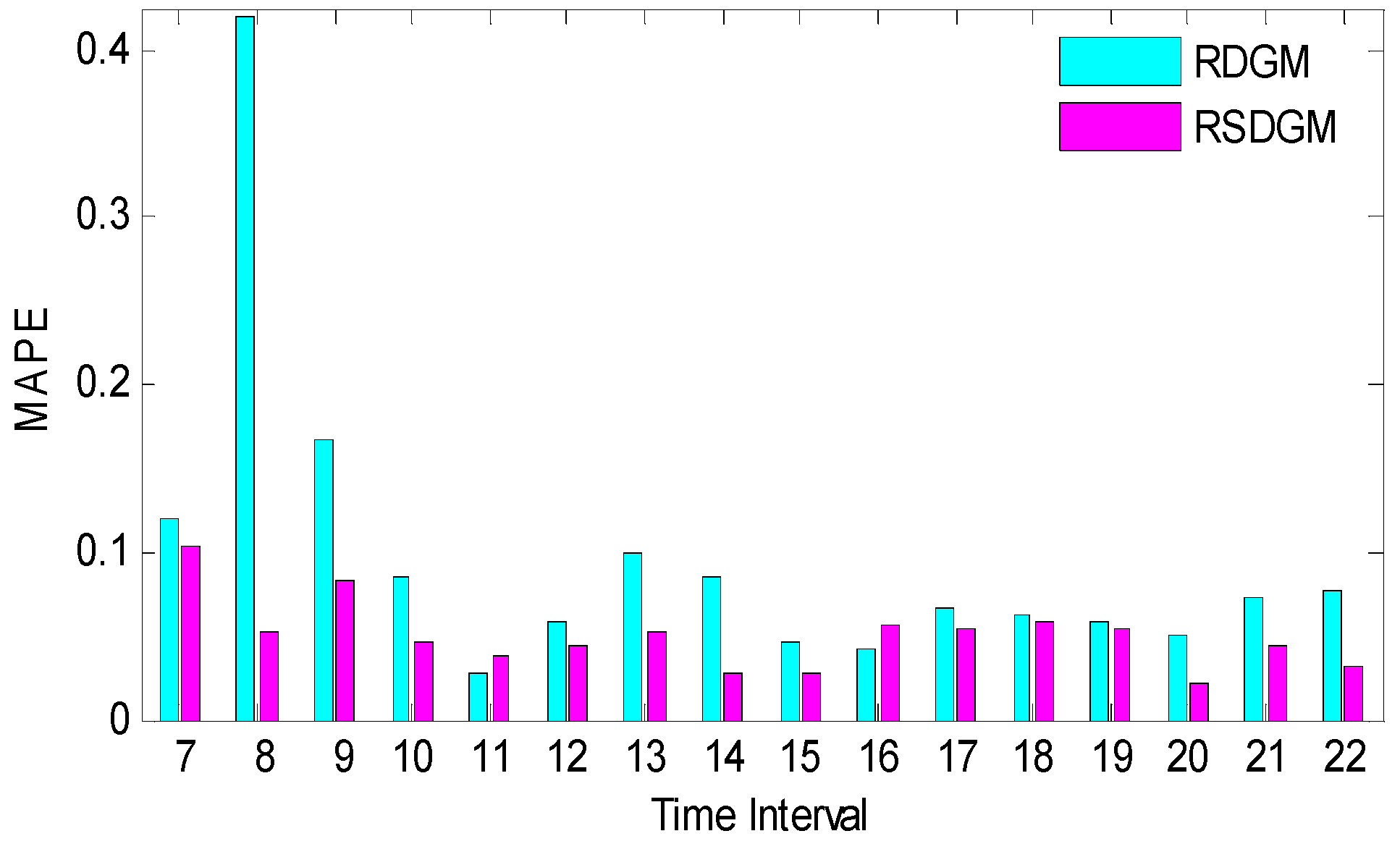
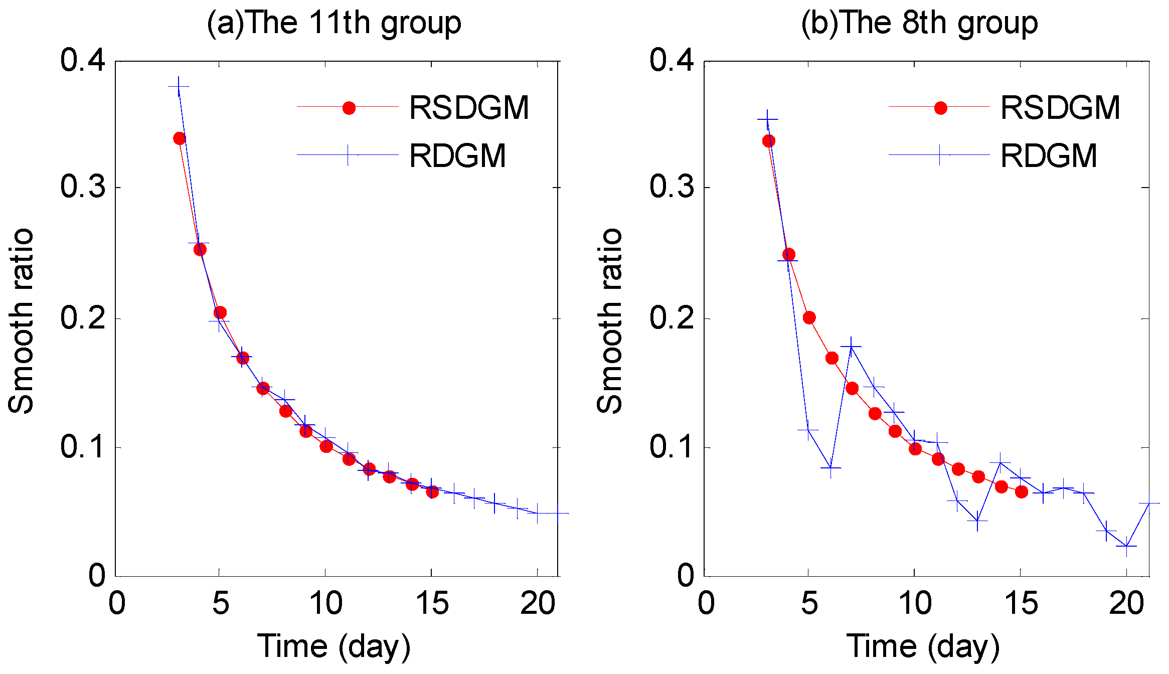
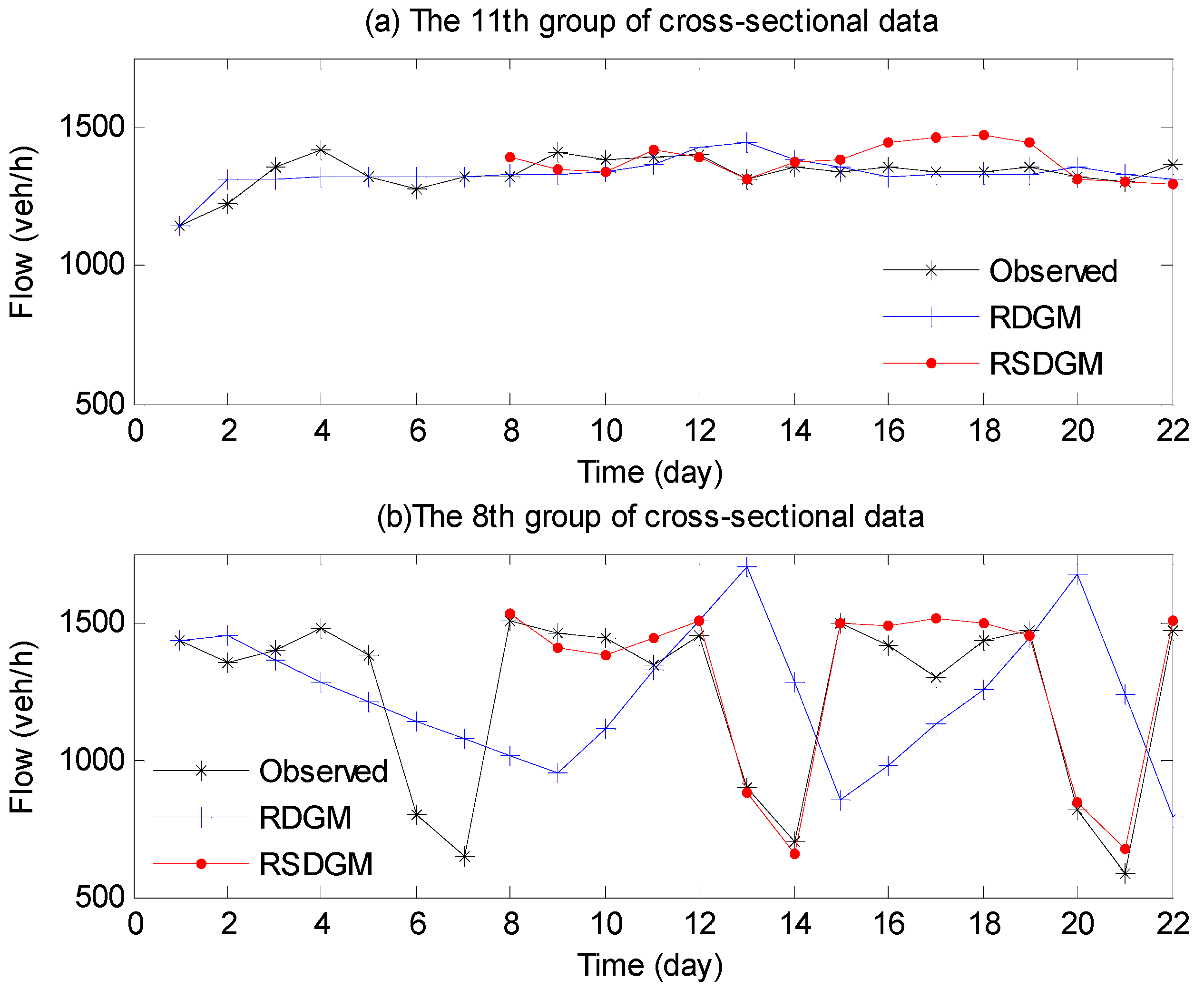
4.2. Analysis of RSDGM(1,1) Model Prediction Results

The RSDGM(1,1) model is used to predict the cross-sectional traffic flow data. From the observed data shown in Figure 4, each set of cross-sectional data has 21 sample values in the training set. As the traffic flow forecasting is mainly for traffic management services, this paper focuses on 16 time intervals from 6:00 to 22:00 each day. Correspondingly, we built 16 RSDGM(1,1) models on 16 different cross-sections. The characteristic of rolling prediction is that in the seven data intervals used for model fitting, after one step prediction, the oldest data point should be removed, and the most recent one should be added. Due to the small amount of computation required, the rolling prediction does not excessively increase the complexity but makes full use of the latest information.

Taking 21 sample values for a cross section as an example, the rolling model was built according to the forecasting procedure shown in Figure 1. For the original sequence $x^{(0)}=(x^{(0)}(1),x^{(0)}(2),\cdots ,x^{(0)}(21))$, q = 7, the Step 1–Step 8 rolling prediction obtained ${\widehat{x}}^{(0)}(14),{\widehat{x}}^{(0)}(15),\cdots ,$ ${\widehat{x}}^{(0)}(21)$. The MAPE of these values was measured as a model performance criterion. The Step 9 rolling prediction obtained ${\widehat{x}}^{(0)}(22)$ compared with the validation data; we calculated the APE of the predicted values for 4 November.

Table 1. Forecast comparison of the RDGM(1,1) and RSDGM(1,1) models.

Cross-Sectional Data Series	Time Interval	RDGM(1,1)		RSDGM(1,1)
		Steps 1–8 Forecast MAPE (%)	4 November Forecast APE (%)	Steps 1–8 Forecast MAPE (%)	4 November Forecast APE (%)
1	6:00–7:00	0.1207	0.3515	0.1028	0.0379
2	7:00–8:00	0.4204	0.4584	0.0519	0.0292
3	8:00–9:00	0.1682	0.2598	0.0839	0.0829
4	9:00–10:00	0.0842	0.1055	0.0453	0.0581
5	10:00–11:00	0.0271	0.0372	0.0383	0.0526
6	11:00–12:00	0.0576	0.0764	0.0434	0.0714
7	12:00–13:00	0.0992	0.0722	0.0525	0.0101
8	13:00–14:00	0.0848	0.1361	0.0286	0.0294
9	14:00–15:00	0.0453	0.0885	0.0278	0.0165
10	15:00–16:00	0.0411	0.0258	0.0560	0.0458
11	16:00–17:00	0.0671	0.0436	0.0541	0.0357
12	17:00–18:00	0.0629	0.0777	0.0580	0.0537
13	18:00–19:00	0.0591	0.0195	0.0545	0.0275
14	19:00–20:00	0.0500	0.1564	0.0224	0.0568
15	20:00–21:00	0.0723	0.0577	0.0435	0.1108
16	21:00–22:00	0.0779	0.0736	0.0326	0.0074

shows the comparative analysis of the RDGM(1,1) and RSDGM(1,1) models for 16 different cross-sectional data intervals. As shown in Figure 5, the RSDGM(1,1) model is better than the DGM(1,1) model in 14 of the 16 sets of cross-sectional data.

Table 2. The distribution of the MAPE values for the RDGM(1,1) and RSDGM(1,1) models.

MAPE	(0%, 3%)	(3%, 6%)	(6%, 10%)	(10%, 50%)
RDGM(1,1)	1	5	7	3
RSDGM(1,1)	3	11	1	1

shows that the RSDGM(1,1) model is more stable than the DGM(1,1) model. In the 16 groups of cross-sectional data, 14 groups had an average relative error of <6%; only 1 group reached 10.28%. However, the average relative error of the RDGM(1,1) model is more discrete; 7 groups were in the range of (6%, 10%), 3 groups exceeded 10%, and the maximum relative error was 42.04%.

Figure 6 shows the smooth ratio of the RDGM(1,1) and RSDGM(1,1) models for the two sets of cross-sectional data. Figure 6a shows that for the 11th set of cross-sectional data, both models met the quasi-smooth conditions and can be used for modeling. Figure 6b shows that the volatility of the 8th set of data was the largest; the RSDGM(1,1) model met the quasi-smooth conditions, and the RDGM(1,1) model did not meet the quasi smooth conditions. The forced modeling results were very poor.

For the periodic volatile data series, comparative analysis shows that the CTAGO operator in the RSDGM(1,1) model can improve the smooth ratio of the sequence to meet the modeling conditions of the quasi-smooth sequence.

Figure 7 shows the prediction effect of the RDGM(1,1) and RSDGM(1,1) models on the two sets of cross-sectional data. In Figure 7a, the daily 1-h traffic flow data in the 10:00–11:00 interval show weaker cycle volatility; however, this situation is rare. In the 16 groups of cross-sectional data, at least 14 groups show strong cycle volatility, as shown in Figure 7b. For the cross-sectional data of the 8th group, the RDGM(1,1) model cannot effectively capture the cyclical fluctuation; thus, the MAPE of the fitting value reached 42.04%. Through the CTAGO operator, the RSDGM(1,1) model can effectively reflect seasonal fluctuation; its MAPE is only 5.19%, which is far better than that of the RDGM(1,1) model. In short, the results of the 16 groups of cross-sectional data analysis show that the RSDGM(1,1) model has better adaptability and stability.

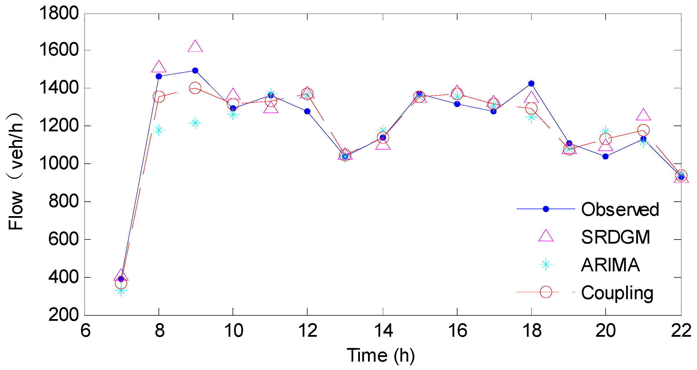
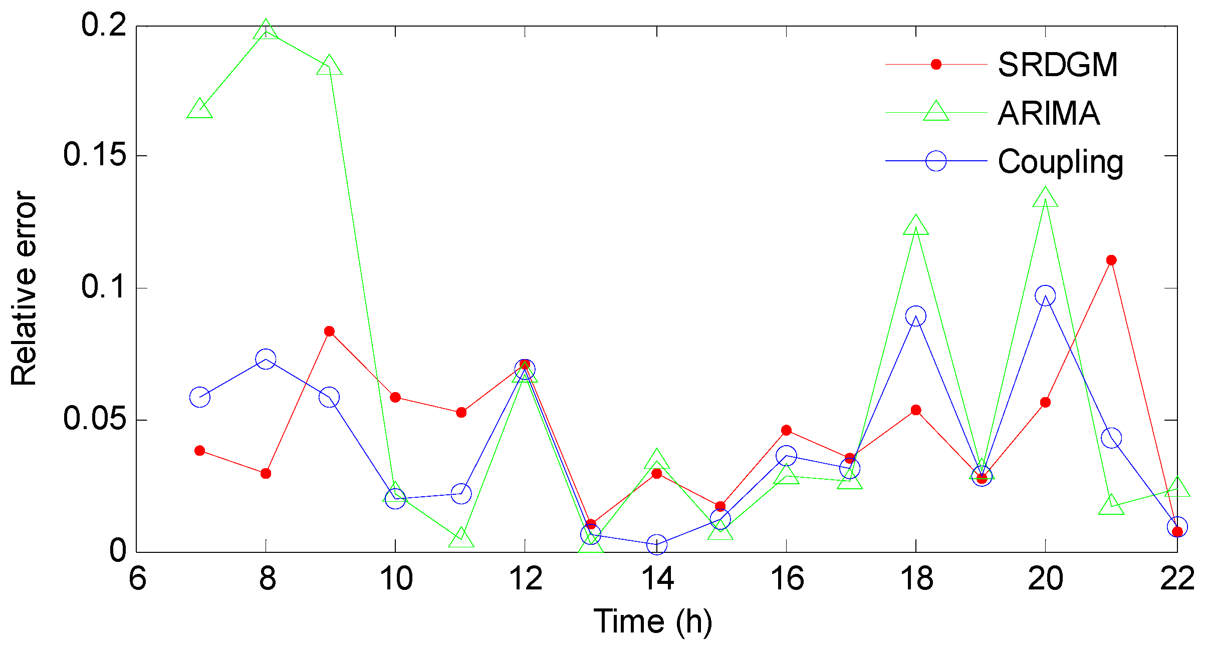
4.3. Analysis of the Coupled Model Prediction Results

In the coupled model based on the nearness grey relational degree, the RSDGM(1,1) model is used to predict the cross-sectional data, and the ARIMA model is used for time-series forecasting. Time-series prediction is based on 504 time interval data points for the historical data set to predict the data for 4 November (Monday). After the test, the original data is not stable, but the first-order difference is stable; thus, the ARIMA(5,1,5) is established. When both transverse and longitudinal models are determined, the coupled prediction model is established in accordance with the algorithm in Section 4.

In the coupled model, the weights are determined by the nearness grey relational degree between the predictive values and the actual values of the $q$ phase before $t+1$ of the single model. The weight of a single model is proportional to the nearness grey relational degree, and the higher the nearness degree is, the greater the weight coefficient is. In a general combination model with the relative errors as the weights, the weights and the errors are inversely proportional; that is, the smaller the error is, the greater the weight is. As shown in Figure 8, the weight coefficients of the RSDGM(1,1) model and the corresponding MAPEs of the 7 time intervals before $t+1$ in the opposite state are consistent with the general combination model. The weight coefficients are in the interval [0.45, 0.650], which reflects the coupled effect of the time-series and cross-sectional data. In the extreme cases, individual coefficients close to 0 or 1 do not appear.

Figure 9 shows the prediction effect of the coupled the ARIMA and RSDGM(1,1) models; the prediction effect of the coupled model is better than that of the two baseline models. Figure 10 shows the relative error of the predicted values of the 3 models in the 16 time intervals for the time period 6:00–22:00 on 4 November. The coupled model clearly improves the prediction effect of the single model: the maximum error is less than 10%, and the average error is reduced to 4.02%. Thus, a stable output is obtained.

Table 3. Comparison of the various model prediction effects.

Model	RSDGM(1,1)	ARIMA	Coupled Model with Equal Weight	Bayesian Combination Model	The Proposed Coupled Model
MAPE	4.54%	6.68%	4.17%	4.44%	4.02%
EC	0.9732	0.9503	0.9738	0.9722	0.9743

shows the prediction results of the 3 models: the coupled model with the nearness grey relational degree, the coupled model with equal weight and the Bayesian combination model. The average relative error of the 3 models is better than that of the single benchmark model, and the optimal result is obtained by the coupled model with the nearness grey relational degree.

5. Conclusions

In this paper, a traffic flow RSDGM-ARIMA coupled prediction model based on time-series and cross-sectional data is established. To account for the weekly seasonality of the cross-sectional data, a new RSDGM(1,1) based on the CTAGO, is developed; a full account of the limited data, nonlinear, and seasonal characteristics of this data is provided. For the coupled process of the time-series and cross-sectional data, a coupled model with a nearness grey relational degree is established, which not only optimizes the prediction precision of the model but also fully considers the performance of the two benchmark models in the coupled model. The smooth ratio condition of the RSDGM model and the rationality of the weight distribution of the coupled model are verified in the numerical experiments. We reach the following conclusions:

(1)

For the weekly seasonality of the cross-sectional traffic flow data, the smooth ratio condition of the DGM(1,1) model is optimized using the CTAGO operator. The experimental results show that the CTAGO sequence can satisfy the quasi-smooth condition when the original seasonal cross-sectional traffic flow data does not. This improvement extends the application scope of the DGM(1,1) model and improves its prediction accuracy.

(2)

A new RSDGM(1,1) based on the CTAGO is established. The CTAGO operator can transform the seasonal fluctuation sequence of the traffic flow into a flat sequence, which can be used to achieve a high precision DGM(1,1) rolling model. Based on matrix perturbation analysis, the length of the sequence in the rolling model is determined, which not only achieves prediction with limited cross-sectional data but also reflects the weight priority of the previous data cycle in the weekly seasonal cross-sectional data.

(3)

A coupled model is established in which the weights are determined by the nearness grey relational degree. By using the nearness grey relational degree to identify the weights, the role of the benchmark model is reflected; moreover, extreme weights do not appear in the intelligent algorithm. The proposed coupled model not only obtains high precision prediction but also considers the performance of the RSDGM(1,1) and ARIMA models in the coupled process.

The improved RSDGM model captures the intra-week seasonal and limited data characteristics of the traffic flow cross-sectional data. Numerical experiments on 16 groups of cross-sectional data show that the RSDGM(1,1) model has good adaptability and stability and can effectively predict the changes in traffic flow. This model is a new attempt to determine the weight of the coupled process based on the nearness grey relational degree. The performance of the coupled model is also better than that of the benchmark model, the coupled model with equal weights and the Bayesian combination model.

References

1. Vlahogianni, E.I.; Karlaftis, M.G.; Golias, J.C. Short-term traffic forecasting: Where we are and where we’re going. Transp. Res. Part C Emerg. Technol. 2014, 43, 3–19. [Google Scholar] [CrossRef]
2. Ran, B.; Jin, P.J.; Boyce, D.; Qiu, T.Z.; Cheng, Y. Perspectives on Future Transportation Research: Impact of Intelligent Transportation System Technologies on Next Generation Transportation Modeling. J. Intell. Transp. Syst. 2012, 16, 226–242. [Google Scholar] [CrossRef]
3. Kamarianakis, Y.; Gao, H.O.; Prastacos, P. Characterizing regimes in daily cycles of urban traffic using smooth-transition regressions. Transp. Res. Part C Emerg. Technol. 2010, 18, 821–840. [Google Scholar] [CrossRef]
4. Sun, H.; Liu, H.; Xiao, H.; He, R.; Ran, B. Use of Local Linear Regression Model for Short-Term Traffic Forecasting. Transp. Res. Rec. J. Transp. Res. Board 2003, 1836, 143–150. [Google Scholar] [CrossRef]
5. Kumar, S.V.; Vanajakshi, L. Short-term traffic flow prediction using seasonal ARIMA model with limited input data. Eur. Transp. Res. Rev. 2015, 7, 1–9. [Google Scholar] [CrossRef]
6. Williams, B.M.; Hoel, L.A. Modeling and forecasting vehicular traffic flow as a seasonal ARIMA process: Theoretical basis and empirical results. J. Transp. Eng. 2003, 129, 664–672. [Google Scholar] [CrossRef]
7. Guo, J.; Huang, W.; Williams, B.M. Adaptive Kalman filter approach for stochastic short-term traffic flow rate prediction and uncertainty quantification. Transp. Res. Part C Emerg. Technol. 2014, 43, 50–64. [Google Scholar] [CrossRef]
8. Guo, H.; Xiao, X.; Forrest, J. Urban road short- term traffic flow forecasting based on the delay and nonlinear grey model. J. Transp. Syst. Eng. Inf. Technol. 2013, 13, 60–66. [Google Scholar] [CrossRef]
9. Mao, S.; Chen, Y.; Xiao, X. City Traffic Flow Prediction Based on Improved GM(1,1) Model. J. Grey Syst. 2012, 24, 337–346. [Google Scholar]
10. Zhang, Y.; Zhang, Y.; Haghani, A. A hybrid short-term traffic flow forecasting method based on spectral analysis and statistical volatility model. Transp. Res. Part C Emerg. Technol. 2014, 43, 65–78. [Google Scholar] [CrossRef]
11. Tchrakian, T.T.; Basu, B.; O’Mahony, M. Real-Time Traffic Flow Forecasting Using Spectral Analysis. IEEE Trans. Intell. Transp. 2012, 13, 519–526. [Google Scholar] [CrossRef]
12. Liu, Y.; Zhang, J. Predicting Traffic Flow in Local Area Networks by the Largest Lyapunov Exponent. Entropy 2016, 18, 32. [Google Scholar] [CrossRef]
13. Ko, E.; Ahn, J.; Kim, E. 3D Markov Process for Traffic Flow Prediction in Real-Time. Sensors 2016, 16, 147. [Google Scholar] [CrossRef] [PubMed]
14. Tan, H.; Wu, Y.; Shen, B.; Jin, P.J.; Ran, B. Short-Term Traffic Prediction Based on Dynamic Tensor Completion. Trans. Intell. Transp. 2016, 17, 2123–2133. [Google Scholar] [CrossRef]
15. Moretti, F.; Pizzuti, S.; Panzieri, S.; Annunziato, M. Urban traffic flow forecasting through statistical and neural network bagging ensemble hybrid modeling. Neurocomputing 2015, 167, 3–7. [Google Scholar] [CrossRef]
16. Huang, M. Intersection traffic flow forecasting based on v-GSVR with a new hybrid evolutionary algorithm. Neurocomputing 2015, 147, 343–349. [Google Scholar] [CrossRef]
17. Hong, W.; Dong, Y.; Zheng, F.; Lai, C. Forecasting urban traffic flow by SVR with continuous ACO. Appl. Math. Model. 2011, 35, 1282–1291. [Google Scholar] [CrossRef]
18. Tang, J.; Zhang, G.; Wang, Y.; Wang, H.; Liu, F.; Tang, J.; Zhang, G.; Wang, Y.; Wang, H.; Liu, F. A hybrid approach to integrate fuzzy C-means based imputation method with genetic algorithm for missing traffic volume data estimation. Transp. Res. Part C Emerg. Technol. 2014, 51, 29–40. [Google Scholar] [CrossRef]
19. Chen, C.; Wang, Y.; Li, L.; Hu, J.; Zhang, Z. The retrieval of intra-day trend and its influence on traffic prediction. Transp. Res. Part C Emerg. Technol. 2012, 22, 103–118. [Google Scholar] [CrossRef]
20. Tang, J.; Wang, H.; Wang, Y.; Liu, X.; Liu, F. Hybrid Prediction Approach Based on Weekly Similarities of Traffic Flow for Different Temporal Scales. Transp. Res. Rec. J. Transp. Res. Board 2014, 2443, 21–31. [Google Scholar] [CrossRef]
21. Zou, Y.; Hua, X.; Zhang, Y. Hybrid short-term freeway speed prediction methods based on periodic analysis. Can. J. Civ. Eng. 2015, 42, 570–582. [Google Scholar] [CrossRef]
22. Barmpadimos, I.; Nufer, M.; Oderbolz, D.C.; Keller, J.; Aksoyoglu, S.; Hueglin, C.; Baltensperger, U.; Prévôt, A.S.H. The weekly cycle of ambient concentrations and traffic emissions of coarse (PM10–PM2.5) atmospheric particles. Atmos. Environ. 2011, 45, 4580–4590. [Google Scholar] [CrossRef]
23. Zhang, N.; Zhang, Y.; Lu, H. Seasonal Autoregressive Integrated Moving Average and Support Vector Machine Models: Prediction of Short-Term Traffic Flow on Freeways. Transp. Res. Rec. J. Transp. Res. Board 2011, 2215, 85–92. [Google Scholar] [CrossRef]
24. Wang, J.; Deng, W.; Guo, Y. New Bayesian combination method for short-term traffic flow forecasting. Transp. Res. Part C Emerg. Technol. 2014, 43, 79–94. [Google Scholar] [CrossRef]
25. Wang, H.; Liu, L.; Qian, Z.; Wei, H.; Dong, S. Empirical Mode Decomposition-Autoregressive Integrated Moving Average. Transp. Res. Rec. J. Transp. Res. Board 2014, 2460, 66–76. [Google Scholar] [CrossRef]
26. Tan, M.; Wong, S.C.; Xu, J.; Guan, Z.; Zhang, P. An Aggregation Approach to Short-Term Traffic Flow Prediction. IEEE Trans. Intell. Transp. 2009, 10, 60–69. [Google Scholar]
27. Qiu, D.G.; Yang, H.Y. A short-term traffic flow forecast algorithm based on double seasonal time series. J. Sichuan Univ. 2013, 45, 64–68. [Google Scholar]
28. Lu, J.; Xie, W.; Zhou, H.; Zhang, A. An optimized nonlinear grey Bernoulli model and its applications. Neurocomputing 2016, 177, 206–214. [Google Scholar] [CrossRef]
29. Yang, Y.; Liu, S.; John, R. Uncertainty Representation of Grey Numbers and Grey Sets. IEEE Trans. Cybern. 2014, 44, 1508–1517. [Google Scholar] [CrossRef] [PubMed] [Green Version]
30. Bezuglov, A.; Comert, G. Short-term freeway traffic parameter prediction: Application of grey system theory models. Expert Syst. Appl. 2016, 62, 284–292. [Google Scholar] [CrossRef]
31. Hosse, R.S.; Becker, U.; Manz, H. Grey Systems Theory Time Series Prediction applied to Road Traffic Safety in Germany. IFAC PapersOnLine 2016, 49, 231–236. [Google Scholar]
32. Xia, M.; Wong, W.K. A seasonal discrete grey forecasting model for fashion retailing. Knowl. Based Syst. 2014, 57, 119–126. [Google Scholar] [CrossRef]
33. Sifeng, L.; Yingjie, Y.; Naiming, X.; Jeffrey, F. New progress of Grey System Theory in the new millennium. Grey Syst. Theory Appl. 2016, 6, 2–31. [Google Scholar]
34. Yuan, C.; Yang, Y.; Chen, D. Proximity and Similitude of Sequences Based on Grey Relational Analysis. J. Grey Syst. 2014, 26, 57–74. [Google Scholar]
35. Zhang, Y.; Ye, N.; Wang, R.; Malekian, R. A Method for Traffic Congestion Clustering Judgment Based on Grey Relational Analysis. ISPRS Int. J. Geo-Inf. 2016, 5, 71. [Google Scholar] [CrossRef]
36. Deng, J.L. Control problems of grey systems. Syst. Control Lett. 1982, 1, 288–294. [Google Scholar]
37. Liu, S.; Lin, Y. Grey Systems: Theory and Applications; Springer: London, UK, 2010; pp. 195–205. [Google Scholar]
38. Xie, N.; Liu, S. Discrete grey forecasting model and its optimization. Appl. Math. Model. 2009, 33, 1173–1186. [Google Scholar] [CrossRef]
39. Ma, X.; Liu, Z. Research on the novel recursive discrete multivariate grey prediction model and its applications. Appl. Math. Model. 2016, 40, 4876–4890. [Google Scholar] [CrossRef]
40. Mao, S.; Gao, M.; Xiao, X.; Zhu, M. A novel fractional grey system model and its application. Appl. Math. Model. 2016, 40, 5063–5076. [Google Scholar] [CrossRef]
41. Shen, Y.; He, B.; Qin, P. Fractional-Order Grey Prediction Method for Non-Equidistant Sequences. Entropy 2016, 18, 227. [Google Scholar] [CrossRef]
42. Akay, D.; Atak, M. Grey prediction with rolling mechanism for electricity demand forecasting of Turkey. Energy 2007, 32, 1670–1675. [Google Scholar] [CrossRef]
43. Zhao, H.; Guo, S. An optimized grey model for annual power load forecasting. Energy 2016, 107, 272–286. [Google Scholar] [CrossRef]
44. Wu, L. Using fractional GM(1,1) model to predict the life of complex equipment. Grey Syst. Theory Appl. 2016, 6, 32–40. [Google Scholar] [CrossRef]
45. Wu, L.; Liu, S.; Fang, Z.; Xu, H. Properties of the GM(1,1) with fractional order accumulation. Appl. Math. Comput. 2015, 252, 287–293. [Google Scholar] [CrossRef]
46. Wu, L.; Liu, S.; Yao, L.; Yan, S. The effect of sample size on the grey system model. Appl. Math. Model. 2013, 37, 6577–6583. [Google Scholar] [CrossRef]
47. Zhang, Q.; Chen, R. Application of metabolic GM(1,1) model in financial repression approach to the financing difficulty of the small and medium-sized enterprises. Grey Syst. Theory Appl. 2014, 4, 311–320. [Google Scholar] [CrossRef]
48. Hamilton, J.D. Time Series Analysis; Princeton University Press: New Jersey, NJ, USA, 1994; pp. 68–70. [Google Scholar]
49. Li, M. Central South University Open ITS Data. Available online: http://www.openits.cn/openPaper/567.jhtml (accessed on 12 July 2016).
Figure 1. Forecasting procedure of RSDGM(1,1) models.
Entropy 18 00454 g001
Figure 2. Flowchart of the coupled forecasting model.
Entropy 18 00454 g002
Figure 3. 3D display of time-series and cross-sectional traffic data.
Entropy 18 00454 g003
Figure 4. Intra-day seasonal traffic trends and intra-week traffic seasonality.
Entropy 18 00454 g004
Figure 5. The MAPE values of the RDGM(1,1) and RSDGM(1,1) models.
Entropy 18 00454 g005
Figure 6. Smooth ratios of the fitting cross-sectional data of two models: (a) the 11th group; (b) the 8th group.
Entropy 18 00454 g006
Figure 7. The prediction effects of the cross-sectional data: (a) the 11th group; (b) the 8th group.
Entropy 18 00454 g007
Figure 8. Comparative analysis of the weights of the RSDGM and the MAPE of the last 7 intervals.
Entropy 18 00454 g008
Figure 9. The prediction effect of the three models for 7:00–22:00 on 4 November.
Entropy 18 00454 g009
Figure 10. The error performance of the prediction results of the 3 models.
Entropy 18 00454 g010