Modelling the Spread of River Blindness Disease via the Caputo Fractional Derivative and the Beta-derivative

Abstract

Information theory is used in many branches of science and technology. For instance, to inform a set of human beings living in a particular region about the fatality of a disease, one makes use of existing information and then converts it into a mathematical equation for prediction. In this work, a model of the well-known river blindness disease is created via the Caputo and beta derivatives. A partial study of stability analysis was presented. The extended system describing the spread of this disease was solved via two analytical techniques: the Laplace perturbation and the homotopy decomposition methods. Summaries of the iteration methods used were provided to derive special solutions to the extended systems. Employing some theoretical parameters, we present some numerical simulations.

1. Introduction

Some of the richest areas in rivers are found in the Tropics. In particular in Africa, the Central and West African countries are blessed with an abundance of rivers. Due to poverty, many residents of these countries rely intensely on these rivers. For instance, it is very common to find that in many villages in Cameroon and Chad, people use rivers as their bathing place and also as their source of drinking water. It is very important to note that water from these rivers is not always healthy and can cause several diseases. One of the most common diseases found in these areas is the so-called onchocerciasis. Onchocerciasis, also called river blindness and Robbes disease is an infectious disease caused by infection with the parasitic worm Onchocerca volvulus [1,2]. This disease is the second most frequent cause of blindness due to infection, after trachoma [1]. In order to accommodate readers that are not familiar with this field, we shall mention that the parasite is spread by the bites of black flies of the genus Simulium (Figure 1) that live near rivers, hence the name of the disease. We shall recall that, once inside a human host, the worm produces larvae that make their way back out to the skin, where they can infect the next black fly that bites that person. An investigation done in [3] showed that usually many bites are required before infection occurs.

An epidemiological study has revealed that about 37 million people are infected with this parasite [4], of which about 300,000 have been permanently blinded [4]. About 99 percent of onchocerciasis cases occur in Africa.

The question that may be asked by readers is perhaps the following: “what does all this have to do with mathematics?” The answer is simple: all phenomena are space and time measurable, so in physical problems, observed facts that perhaps cannot be measured exactly can be approximated after conversion into a mathematical formula. The aim of this paper is therefore based on the mathematical aspects of the disease, in particular the model underpinning the spread of this disease. We shall present this model utilizing fractional derivatives. The reason for using fractional derivatives can be found in many recently published papers in the area of mathematical modelling [5,6,7,8,9]. The physical interpretation of the fractional derivative concept can be found in [10].

Figure 1. Female black fly biting a human being.

Figure 1. Female black fly biting a human being.

The mathematical model under consideration here is given as:

$$\{\begin{array}{c}\frac{d{H}_s(t)}{dt}=\psi +{\delta }_H{V}_I+\alpha \beta H_I-\xi H_S{V}_I-{\tau }_H{H}_S\\ \frac{d{H}_I(t)}{dt}=H_S{V}_I-{\delta }_I{H}_I-\alpha \beta H_I-\xi H_S{V}_I-{\tau }_I{H}_I\\ \frac{d{V}_V(t)}{dt}={\delta }_V{H}_I-{\rho }_I{V}_I-\gamma V_S\\ \frac{d{V}_S(t)}{dt}=\delta V_S-{\rho }_I{V}_I-{\delta }_H{V}_I\end{array}$$

(1)

With the advantages offered by the concept of fractional derivative and other newly proposed derivatives, in this paper we shall extend this model within the scope of fractional derivatives as well as the beta-derivative. Therefore Equation (1) can be converted into the following:

$$\{\begin{array}{c}{}_0{}^{A}D_t^{\alpha }{H}_s(t)=\psi +{\delta }_H{V}_I+\alpha \beta H_I-\xi H_S{V}_I-{\tau }_H{H}_S\\ {}_0{}^{A}D_t^{\alpha }{H}_l(t)=H_S{V}_I-{\delta }_I{H}_I-\alpha \beta H_I-\xi H_S{V}_I-{\tau }_I{H}_I\\ {}_0{}^{A}D_t^{\alpha }{V}_I(t)={\delta }_V{H}_I-{\rho }_I{V}_I-\gamma V_S\\ {}_0{}^{A}D_t^{\alpha }{V}_S(t)=\delta V_S-{\rho }_I{V}_I-{\delta }_H{V}_I \end{array}$$

(2)

where, ${}_0{}^{A}D_t^{\alpha }$ is the Caputo derivative or the new derivative called beta-derivative. We shall give in the next section some background relating the use of fractional and beta-derivatives. The aim of this paper is a comparative study of the beta and fractional derivative for modeling epidemiological problems. The fractional derivative is mostly used for non-local problems and maybe not suitable for epidemiological problems. However the fractional order plays an important role in numerical simulations, therefore a local derivative with fractional order is introduced in this paper to model the spread of river blindness disease.

2. Some Information about the Beta-Derivative and Caputo Derivative

Definition 1. 

Let $f$ be a function, such that, $f:[a, \infty )\to ℝ$. Then the beta-derivative is defined as:

$${}_0{}^{A}D_x^{\beta }(f(x))=\underset{\epsilon \to 0}{\lim }\frac{f(x+\epsilon {(x+\frac{1}{\text{Γ}(\beta )})}^{1-\beta })-f(x)}{\epsilon }$$

(3)

for all $x\ge a, \beta \in (0,1]$. Then is the limit of the above exists, f is says to be beta-differentiable.

One can remark that, the above definition does not depend on the interval. If the function is differentiable, our definition at a point zero is different from zero.

Theorem 1. 

Assuming that, $g\ne 0$ and f are two functions beta-differentiable with $\beta \in (0,1]$ then, the following relations can be satisfied:

• $1-{}_0{}^{A}D_x^{\alpha }(af(x)+bg(x))=a{}_0{}^{A}D_x^{\alpha }(f(x))+b{}_0{}^{A}D_x^{\alpha }(f(x))$ for all a and b real number,
• $2-{}_0{}^{A}D_x^{\alpha }(c)=0$ for c any given constant,
• $3-{}_0{}^{A}D_x^{\alpha }(f(x)g(x))=g(x){}_0{}^{A}D_x^{\alpha }(f(x))+f(x){}_0{}^{A}D_x^{\alpha }(g(x))$,
• $4-{}_0{}^{A}D_x^{\alpha }(\frac{f(x)}{g(x)})=\frac{g(x){}_0{}^{A}D_x^{\alpha }(f(x))-f(x){}_{}{}^0{}_{A}D_x^{\alpha }{}_{}(g(x))}{g^2(x)}$.

The proofs of the above relations are the same as the one in [11].

Theorem 2. 

Asuming that $f:[a, \infty )\to ℝ$, be a functions such that, $f$ is differentiable and also alpha-differentiable. Let g be a function defined in the range of $f$ and also differentiable, then we have the following rule:

$${}_0{}^{A}D_x^{\beta }(gof(x))={(x+\frac{1}{\text{Γ}(\beta )})}^{1-\beta }{f}^{\prime }(x)g^{\prime }(f(x))$$

(4)

Definition 2. 

Let $f:[a, \infty )\to ℝ$ is given function, then we propose that the beta-integral of $f$ is:

$${}_a{}^{A}I_x^{\beta }(f(x))=\underset{a}{\overset{x}{{\displaystyle \int }}}{(t+\frac{1}{\text{Γ}(\beta )})}^{\beta -1}f(t)dt$$

(5)

The above operator is the inverse operator of the proposed fractional derivative. We shall present to underpin this statement by the following theorem.

Theorem 3. 

${}_0{}^{A}D_x^{\alpha }\left[{}_0{}^{A}I_x^{\alpha }f(x)\right]=f(x)$ for all $x \ge a$ with f a given continuous and differentiable function.

Definition 3. 

The Caputo fractional derivative of a differentiable function is defined as:

$$D_x^{\alpha }(f(x))=\frac{1}{\text{Γ}(n-\alpha )}\underset{0}{\overset{x}{{\displaystyle \int }}}{(x-t)}^{n-\alpha -1}{(\frac{d}{dt})}^{n}f(t)dt, n-1<\alpha \le n$$

(6)

The properties underpinning the use of the Caputo derivative can be found in [5,6,7,8,9]. With all this information in hand, we shall present in the next section the analysis of this model.

3. Analysis of the Mathematical Model

In this section, we present a discussion strengthening the stability analysis of the model and via two methods. One will be with the concept of eigenvalues and the other one will be via the reproductive number. One of the advantages of the Caputo and beta-derivative is that, if the function is a constant, then the Caputo and the beta-derivative of that function give zero. We can therefore make use of these properties to find the disease-free equilibrium point and the endemic equilibrium points. At the equilibrium points, we assume that the system does not depend on time, therefore ${}_0{}^{A}D_t^{\alpha }{H}_s(t)={}_0{}^{A}D_t^{\alpha }{H}_l(t)={}_0{}^{A}D_t^{\alpha }{V}_I(t)={}_0{}^{A}D_t^{\alpha }{V}_S(t)=0$ such that:

$$\{\begin{array}{c}0=\psi +{\delta }_H{\overline{V}}_I+\alpha \beta \overline{H_I}-\xi H_S{\overline{V}}_I-{\tau }_H\overline{H_S}\\ 0=\overline{H_S}{\overline{V}}_I-{\delta }_I{\overline{H}}_I-\alpha \beta \overline{H_I}-\xi H_S{\overline{V}}_I-{\tau }_I{\overline{H}}_I\\ 0={\delta }_V\overline{H_I}-{\rho }_I{\overline{V}}_I-\gamma \overline{V_S }\\ 0=\delta {\overline{V}}_S-{\rho }_I{\overline{V}}_I-{\delta }_H\overline{V_I } \end{array}$$

Solving the above system, we obtain first:

$${\overline{V}}_I=\frac{\delta {\overline{V}}_S}{\rho +{\delta }_H}, {\overline{H}}_I=(\frac{{\rho }_1\delta }{\rho +{\delta }_H}-\gamma ){\overline{V}}_S$$

(7)

However, introducing these equations in the system, we obtain the following:

$$\begin{array}{c}{\overline{V}}_I=\frac{\psi \xi \gamma {\delta }_V-{\tau }_H({\rho }_S+\gamma )({\rho }_I+{\delta }_H)(\alpha \beta +{\tau }_I+\sigma +{\delta }_V)}{\gamma \left[\xi ({\rho }_I+{\delta }_H)({\rho }_s+\gamma )({\tau }_I+\gamma )+{\delta }_V{\rho }_S\right]+\xi \gamma {\rho }_I {\delta }_V}\\ {\overline{V}}_S=\frac{({\rho }_I+{\delta }_H)\left[\psi \xi \gamma {\delta }_V-{\tau }_H({\rho }_s+\gamma )({\rho }_I+{\delta }_H)(\alpha \beta +{\tau }_I+\sigma +{\delta }_V)\right]}{\gamma \left[\xi ({\rho }_I+{\delta }_H)\left[({\rho }_s+\gamma )({\tau }_I+\sigma )\right]+\xi +{\rho }_I{\delta }_V\right]+\xi \gamma {\rho }_I {\delta }_V}\\ {\overline{H}}_I=\frac{({\rho }_S+\gamma )({\rho }_I+{\delta }_H)\left[\psi \xi \gamma {\delta }_V-{\tau }_H({\rho }_s+\gamma )({\rho }_I+{\delta }_H)(\alpha \beta +{\tau }_I+\sigma +{\delta }_V)\right]}{\gamma {\delta }_V\left[\xi ({\rho }_I+{\delta }_H)\left[({\rho }_s+\gamma )({\tau }_I+\sigma )\right]+\xi +{\rho }_I{\delta }_V\right]+\xi \gamma {\rho }_I {\delta }_V}\\ {\overline{H}}_S=\frac{({\rho }_S+\gamma )({\rho }_I+{\delta }_H)\alpha \beta +{\tau }_I+\sigma +{\delta }_V}{\xi \gamma {\delta }_V}\end{array}$$

(8)

Hence the disease-free equilibrium is given as:

$$({\overline{H}}_S,{\overline{H}}_I,{\overline{V}}_S,{\overline{V}}_I)=(\frac{\psi }{{\tau }_H},0,0,0)$$

(9)

The stability analysis of this system has been investigated in [12]. Our next concern will be to provide an approximate solution with two analytical techniques for each case.

4. Analysis of Approximate Solutions

One of the most difficult tasks in non-linear fractional differential equation systems is perhaps the derivation of exact analytical solutions. That is why in the recent decades, several studies have been done in order to build some analytical techniques that can be used to provide asymptotic solutions in such systems. We shall mention some of the recent and efficient ones that have been intensively used, such as the homotopy perturbation method [11,13], the Adomian Decomposition method [14,15], the homotopy Laplace perturbation method [16], the Sumudu homotopy perturbation method [17] and the homotopy decomposition method [18]. However, in this paper we shall use only two of these mentioned techniques, namely the Laplace homotopy perturbation method and the homotopy decomposition method. The homotopy decomposition method will be used to solve the system with the beta-derivative and then, the Laplace homotopy perturbation method will be used to provide the solution of the system with Caputo derivative.

4.1. Solution with the Laplace Homotopy Perturbation Method

This version was first proposed in [16] and has been also used in other research. We shall present the methodology for solving system (2) with the Caputo fractional derivative:

$$\{\begin{array}{c}{}_0{}^{C}D_t^{\alpha }{H}_s(t)=\psi +{\delta }_H{V}_I+\alpha \beta H_I-\xi H_S{V}_I-{\tau }_H{H}_S\\ {}_0{}^{C}D_t^{\alpha }{H}_l(t)=H_S{V}_I-{\delta }_I{H}_I-\alpha \beta H_I-\xi H_S{V}_I-{\tau }_I{H}_I\\ {}_0{}^{C}D_t^{\alpha }{V}_I(t)={\delta }_V{H}_I-{\rho }_I{V}_I-\gamma V_S\\ {}_0{}^{C}D_t^{\alpha }{V}_S(t)=\delta V_S-{\rho }_I{V}_I-{\delta }_H{V}_I\end{array}$$

An application of the Laplace transform operator on both sides of the above system leads us to the following:

$$\{\begin{array}{c}{H}_s(\tau )=\frac{1}{{\tau }^{\alpha }}{H}_s(0)+\frac{1}{{\tau }^{\alpha }}ℒ(\psi +{\delta }_H{V}_I+\alpha \beta H_I-\xi H_S{V}_I-{\tau }_H{H}_S)\\ H_l(\tau )=\frac{1}{{\tau }^{\alpha }}{H}_l(0)+\frac{1}{{\tau }^{\alpha }}ℒ(H_S{V}_I-{\delta }_I{H}_I-\alpha \beta H_I-\xi H_I{V}_I-{\tau }_I{H}_I)\\ V_I(\tau )=\frac{1}{{\tau }^{\alpha }}{V}_I(0)+\frac{1}{{\tau }^{\alpha }}ℒ({\delta }_V{H}_I-{\rho }_I{V}_I-\gamma V_S)\\ V_S(\tau )=\frac{1}{{\tau }^{\alpha }}{V}_S(0)+\frac{1}{{\tau }^{\alpha }}ℒ(\delta V_S-{\rho }_I{V}_I-{\delta }_H{V}_I)\end{array}$$

(10)

here, $\tau$ is the Laplace variable. An addition application of the inverse Laplace transform on both sides of the system yields:

$$\{\begin{array}{c}{H}_s(t)=H_s(0)+{ℒ}^{-1}\left\{\frac{1}{{\tau }^{\alpha }}ℒ(\psi +{\delta }_H{V}_I+\alpha \beta H_I-\xi H_S{V}_I-{\tau }_H{H}_S)\right\}\\ H_l(t)=H_l(0)+{ℒ}^{-1}\left\{\frac{1}{{\tau }^{\alpha }}ℒ(H_S{V}_I-{\delta }_I{H}_I-\alpha \beta H_I-\xi H_I{V}_I-{\tau }_I{H}_I)\right\}\\ V_I(t)=V_I(0)+{ℒ}^{-1}\left\{\frac{1}{{\tau }^{\alpha }}ℒ({\delta }_V{H}_I-{\rho }_I{V}_I-\gamma V_S)\right\}\\ V_S(t)=V_S(0)+{ℒ}^{-1}\left\{\frac{1}{{\tau }^{\alpha }}ℒ(\delta V_S-{\rho }_I{V}_I-{\delta }_H{V}_I)\right\}\end{array}$$

(11)

With the above system in hand, we shall assume that a solution of the above can be obtained in series form as follows:

$$H_s(t)={\displaystyle \sum }_{n=0}^{\infty }{H}_{sn}(t), H_I(t)={\displaystyle \sum }_{n=0}^{\infty }{H}_{In}(t), V_s(t)={\displaystyle \sum }_{n=0}^{\infty }{V}_{sn}(t), V_I(t)={\displaystyle \sum }_{n=0}^{\infty }{V}_{In}(t)$$

(12)

However, replacing the above solution in system (11) and including the embedding parameter $p\in (0,1]$, putting together all the terms of the same power of the embedding parameter p we obtain:

$$p^0:\{\begin{array}{c}{H}_{s0}(t)=H_s(0)\\ H_{l0}(t)=H_l(0)\\ V_{I0}(t)=V_I(0)\\ V_{S0}(t)=V_S(0) \end{array}$$

(13)

$$p^1:\{\begin{array}{c}{H}_{s1}(t)={ℒ}^{-1}\left\{\frac{1}{{\tau }^{\alpha }}ℒ(\psi +{\delta }_H{V}_{I0}+\alpha \beta H_{I0}-\xi H_{S0}{V}_{I0}-{\tau }_H{H}_{S0})\right\}\\ H_{l1}(t)={ℒ}^{-1}\left\{\frac{1}{{\tau }^{\alpha }}ℒ(H_{S0}{V}_{I0}-{\delta }_I{H}_{I0}-\alpha \beta H_{I0}-\xi H_{I0}{V}_{I0}-{\tau }_I{H}_{I0})\right\}\\ V_{I1}(t)={ℒ}^{-1}\left\{\frac{1}{{\tau }^{\alpha }}ℒ({\delta }_V{H}_{0I}-{\rho }_I{V}_{I0}-\gamma V_{S0})\right\}\\ V_{S1}(t)={ℒ}^{-1}\left\{\frac{1}{{\tau }^{\alpha }}ℒ(\delta V_{S0}-{\rho }_I{V}_{I0}-{\delta }_H{V}_{I0})\right\}\end{array}$$

In general, we shall have the following system of iteration formulas (14):

$$p^n:\{\begin{array}{c}{H}_{sn}(t)={ℒ}^{-1}\left\{\frac{1}{s^{\alpha }}ℒ(\psi +{\delta }_H{V}_{I(n-1)}+\alpha \beta H_{I(n-1)}-\xi {\displaystyle {\displaystyle \sum }_{j=0}^{n-1}}{V}_{I(n-j-1)}{H}_{Sj}-{\tau }_H{H}_{S(n-1)})\right\}\\ H_{l1}(t)={ℒ}^{-1}\left\{\frac{1}{s^{\alpha }}ℒ({\displaystyle {\displaystyle \sum }_{j=0}^{n-1}}{V}_{I(n-j-1)}{H}_{Sj} -{\delta }_I{H}_{I(n-1)}-\alpha \beta H_{I(n-1)}-\xi {\displaystyle {\displaystyle \sum }_{j=0}^{n-1}}{V}_{I(n-j-1)}{H}_{Ij}-{\tau }_I{H}_{I(n-1)})\right\}\\ V_{I1}(t)={ℒ}^{-1}\left\{\frac{1}{s^{\alpha }}ℒ({\delta }_V{H}_{I(n-1)}-{\rho }_I{V}_{I(n-1)}-\gamma V_{S(n-1)})\right\}\\ V_{S1}(t)={ℒ}^{-1}\left\{\frac{1}{s^{\alpha }}ℒ(\delta V_{S(n-1)}-{\rho }_I{V}_{I(n-1)}-{\delta }_H{V}_{I(n-1)})\right\}\end{array}$$

(14)

The above development can be summarized in the following algorithm:

Algorithm 1. This procedure can be used to derive a special solution to system (2) with a Caputo fractional derivative:

Input: $\{\begin{array}{c}{\text{H}}_{\text{s}0}(\text{t})={\text{H}}_{\text{s}}(0)\\ {\text{H}}_{\text{l}0}(\text{t})={\text{H}}_{\text{l}}(0)\\ {\text{V}}_{\text{I}0}(\text{t})={\text{V}}_{\text{I}}(0)\\ {\text{V}}_{\text{S}0}(\text{t})={\text{V}}_{\text{S}}(0) \end{array}$ as preliminary input, $j-$number terms in the rough calculation, Output: $\{\begin{array}{c}{H}_{sappr}(t)\\ H_{lappr}(t)\\ V_{Iappr}(t)\\ V_{Sappr}(t) \end{array}$, the approximate solution.

Step 1: Put $\{\begin{array}{c}{H}_{s0}(t)=H_s(t)\\ H_{l0}(t)=H_l(0)\\ V_{I0}(t)=V_I(0)\\ V_{S0}(t)=V_S(0)\end{array}$ and $\{\begin{array}{c}{H}_{sappr}(t)\\ H_{lappr}(t)\\ V_{Iappr}(t)\\ V_{Sappr}(t)\end{array}=\{\begin{array}{c}{H}_{s0}(t)\\ H_{l0}(t)\\ V_{I0}(t)\\ V_{S0}(t).\end{array}$,

Step 2: For $j=1$ to $n-1$ do step 3, step 4 and step 5: $$\{\begin{array}{c}{H}_{s1}(t)={ℒ}^{-1}\left\{\frac{1}{{\tau }^{\alpha }}ℒ(\psi +{\delta }_H{V}_{I0}+\alpha \beta H_{I0}-\xi H_{S0}{V}_{I0}-{\tau }_H{H}_{S0})\right\}\\ H_{l1}(t)={ℒ}^{-1}\left\{\frac{1}{{\tau }^{\alpha }}ℒ(H_{S0}{V}_{I0}-{\delta }_I{H}_{I0}-\alpha \beta H_{I0}-\xi H_{I0}{V}_{I0}-{\tau }_I{H}_{I0})\right\}\\ V_{I1}(t)={ℒ}^{-1}\left\{\frac{1}{{\tau }^{\alpha }}ℒ({\delta }_V{H}_{0I}-{\rho }_I{V}_{I0}-\gamma V_{S0})\right\}\\ V_{S1}(t)={ℒ}^{-1}\left\{\frac{1}{{\tau }^{\alpha }}ℒ(\delta V_{S0}-{\rho }_I{V}_{I0}-{\delta }_H{V}_{I0})\right\}\end{array}.$$

Step 3: Compute: $$\{\begin{array}{c}{B}_{sn}(t)={ℒ}^{-1}\left\{\frac{1}{{\tau }^{\alpha }}ℒ(\psi +{\delta }_H{V}_{I(n-1)}+\alpha \beta H_{I(n-1)}-\xi {\displaystyle {\displaystyle \sum }_{j=0}^{n-1}}{V}_{I(n-j-1)}{H}_{Sj}-{\tau }_H{H}_{S(n-1)})\right\}\\ B_{ln}(t)={ℒ}^{-1}\left\{\frac{1}{{\tau }^{\alpha }}ℒ({\displaystyle {\displaystyle \sum }_{j=0}^{n-1}}{V}_{I(n-j-1)}{H}_{Sj}-{\delta }_I{H}_{I(n-1)}-\alpha \beta H_{I(n-1)}-\xi {\displaystyle {\displaystyle \sum }_{j=0}^{n-1}}{V}_{I(n-j-1)}{H}_{Ij}-{\tau }_I{H}_{I(n-1)})\right\}\\ K_{In}(t)={ℒ}^{-1}\left\{\frac{1}{{\tau }^{\alpha }}ℒ({\delta }_V{H}_{I(n-1)}-{\rho }_I{V}_{I(n-1)}-\gamma V_{S(n-1)})\right\}\\ K_{Sn}(t)={ℒ}^{-1}\left\{\frac{1}{{\tau }^{\alpha }}ℒ(\delta V_{S(n-1)}-{\rho }_I{V}_{I(n-1)}-{\delta }_H{V}_{I(n-1)})\right\}.\end{array}$$

Step 4: Compute: $$\{\begin{array}{c}{H}_{s(m+1)}(t)=B_{ms}(t)+H_{s(appr)}(t)\\ H_{l(m+1)}(t)=B_{ml}(t)+H_{l(appr)}(t)\\ V_{I(m+1)}(t)=K_{Im}(t)+V_{I(appr)}(t)\\ V_{S(m+1)}(t)=K_{Sm}(t)+V_{S(appr)}(t)\end{array},$$

Step 5: Compute: $$\{\begin{array}{l}{H}_{s(appr)}(t)=H_{apprS}(t)+H_{s(m+1)}(t)\\ H_{l(appr)}(t)=H_{lappr}(t)+H_{l(m+1)}(t)\\ V_{I(appr)}(t)=V_{Iappr}(t)+V_{I(m+1)}(t)\\ V_{S(appr)}(t)=V_{Sappr}(t)+V_{S(m+1)}(t).\end{array}$$

Stop.

The above algorithm shall be used to derive the special solution of system (2) with the Caputo derivative. We shall examine the case where the beta-derivative and this are done in the following Section 4.2.

4.2. Solution with the Homotopy Decomposition Method

This technique is used here to derive a special solution to system (2) with the beta-derivative because the application of the Laplace transform on this derivative does not give satisfactory results. However, we can apply the inverse operator of this derivative, which is referred to as the beta-integral, in order to transform the ordinary differential equation into an integral equation such that the idea of homotopy can employed. Therefore applying the inverse operator on both sides of system (2), we obtain the following system of integral equations:

$$\{\begin{array}{c}{H}_s(\tau )=H_s(0)+{}_0{}^{A}I_t^{\alpha }(\psi +{\delta }_H{V}_I+\alpha \beta H_I-\xi H_S{V}_I-{\tau }_H{H}_S)\\ H_l(\tau )=H_l(0)+{}_0{}^{A}I_t^{\alpha }(H_S{V}_I-{\delta }_I{H}_I-\alpha \beta H_I-\xi H_I{V}_I-{\tau }_I{H}_I)\\ V_I(\tau )=V_I(0)+{}_0{}^{A}I_t^{\alpha }({\delta }_V{H}_I-{\rho }_I{V}_I-\gamma V_S)\\ V_S(\tau )=V_S(0)+{}_0{}^{A}I_t^{\alpha }(\delta V_S-{\rho }_I{V}_I-{\delta }_H{V}_I)\end{array}$$

(15)

where:

$${}_0{}^{A}I_t^{\beta }(f(t))=\underset{0}{\overset{t}{{\displaystyle \int }}}{(\tau +\frac{1}{\text{Γ}(\beta )})}^{1-\beta }f(\tau )d\tau$$

(16)

In addition to this, we shall assume that a solution of the above can be obtained in series form as follows:

$$H_s(t)={\displaystyle \sum }_{n=0}^{\infty }{H}_{sn}(t), H_I(t)={\displaystyle \sum }_{n=0}^{\infty }{H}_{In}(t), V_s(t)={\displaystyle \sum }_{n=0}^{\infty }{V}_{sn}(t), V_I(t)={\displaystyle \sum }_{n=0}^{\infty }{V}_{In}(t)$$

(17)

However, replacing the above solution in system (15) and including the embedding parameter $p\in (0,1]$, putting together all the terms of the same power of the embedding parameter p we obtain:

$$\{\begin{array}{c}{H}_{s0}(t)=H_s(0)\\ H_{l0}(t)=H_l(0)\\ V_{I0}(t)=V_I(0)\\ V_{S0}(t)=V_S(0) \end{array}$$

(18)

$p^1:\{\begin{array}{c}{H}_{s1}(t)=\underset{0}{\overset{t}{{\displaystyle \int }}}{(\tau +\frac{1}{\text{Γ}(\beta )})}^{1-\beta }\left\{\psi +{\delta }_H{V}_{I0}+\alpha \beta H_{I0}-\xi H_{S0}{V}_{I0}-{\tau }_H{H}_{S0}\right\}d\tau \\ H_{l1}(t)=\underset{0}{\overset{t}{{\displaystyle \int }}}{(\tau +\frac{1}{\text{Γ}(\beta )})}^{1-\beta }\left\{H_{S0}{V}_{I0}-{\delta }_I{H}_{I0}-\alpha \beta H_{I0}-\xi H_{I0}{V}_{I0}-{\tau }_I{H}_{I0}\right\}d\tau \\ V_{I1}(t)=\underset{0}{\overset{t}{{\displaystyle \int }}}{(\tau +\frac{1}{\text{Γ}(\beta )})}^{1-\beta }({\delta }_V{H}_{0I}-{\rho }_I{V}_{I0}-\gamma V_{S0}) d\tau \\ V_{S1}(t)=\underset{0}{\overset{t}{{\displaystyle \int }}}{(\tau +\frac{1}{\text{Γ}(\beta )})}^{1-\beta }\left\{\delta V_{S0}-{\rho }_I{V}_{I0}-{\delta }_H{V}_{I0}\right\}d\tau \end{array}$

In general, we shall have the following system of iteration formulas:

$$p^n:\{\begin{array}{c}{H}_{sn}(t)=\underset{0}{\overset{t}{{\displaystyle \int }}}{(\tau +\frac{1}{\text{Γ}(\beta )})}^{1-\beta }\left\{\psi +{\delta }_H{V}_{I(n-1)}+\alpha \beta H_{I(n-1)}-\xi {\displaystyle {\displaystyle \sum }_{j=0}^{n-1}}{V}_{I(n-j-1)}{H}_{Sj}-{\tau }_H{H}_{S(n-1)}\right\}d\tau \\ H_{l1}(t)=\underset{0}{\overset{t}{{\displaystyle \int }}}{(\tau +\frac{1}{\text{Γ}(\beta )})}^{1-\beta }\left\{{\displaystyle {\displaystyle \sum }_{j=0}^{n-1}}{V}_{I(n-j-1)}{H}_{Sj}-{\delta }_I{H}_{I(n-1)}-\alpha \beta H_{I(n-1)}-\xi {\displaystyle {\displaystyle \sum }_{j=0}^{n-1}}{V}_{I(n-j-1)}{H}_{Ij}-{\tau }_I{H}_{I(n-1)}\right\}d\tau \\ V_{I1}(t)=\underset{0}{\overset{t}{{\displaystyle \int }}}{(\tau +\frac{1}{\text{Γ}(\beta )})}^{1-\beta }\left\{H_{I(n-1)}-{\rho }_I{V}_{I(n-1)}-\gamma V_{S(n-1)}\right\} d\tau \\ V_{S1}(t)=\underset{0}{\overset{t}{{\displaystyle \int }}}{(\tau +\frac{1}{\text{Γ}(\beta )})}^{1-\beta }\left\{\delta V_{S(n-1)}-{\rho }_I{V}_{I(n-1)}-{\delta }_H{V}_{I(n-1)}\right\}d\tau \end{array}$$

(19)

The overhead elaboration can be restarted in the succeeding procedure.

Algorithm 2. This procedure can be used to derive a special solution to the system two with Atangana’s $\beta$-derivative:

Input: $\{\begin{array}{c}{H}_{s0}(t)=H_s(0)\\ H_{l0}(t)=H_l(0)\\ V_{I0}(t)=V_I(0)\\ V_{S0}(t)=V_S(0)\end{array}$ as preliminary input, $j-$number terms in the rough calculation, Output: $\{\begin{array}{c}{H}_{sappr}(t)\\ H_{lappr}(t)\\ V_{Iappr}(t)\\ V_{Sappr}(t) \end{array}$, the approximate solution.

Step 1: Put $\{\begin{array}{c}{H}_{s0}(t)=H_s(t)\\ H_{l0}(t)=H_l(0)\\ V_{I0}(t)=V_I(0)\\ V_{S0}(t)=V_S(0) \end{array}$ and $\{\begin{array}{c}{H}_{sappr}(t)\\ H_{lappr}(t)\\ V_{Iappr}(t)\\ V_{Sappr}(t) \end{array}= \{\begin{array}{c}{H}_{s0}(t)\\ H_{l0}(t)\\ V_{I0}(t)\\ V_{S0}(t). \end{array}$,

Step 2: For $j=1$ to $n-1$ do step 3, step 4 and step 5: $$\{\begin{array}{c}{H}_{s1}(t)=\underset{0}{\overset{t}{{\displaystyle \int }}}{(\tau +\frac{1}{\text{Γ}(\beta )})}^{1-\beta }\left\{\psi +{\delta }_H{V}_{I0}+\alpha \beta H_{I0}-\xi H_{S0}{V}_{I0}-{\tau }_H{H}_{S0}\right\}d\tau \\ H_{l1}(t)=\underset{0}{\overset{t}{{\displaystyle \int }}}{(\tau +\frac{1}{\text{Γ}(\beta )})}^{1-\beta }\left\{H_{S0}{V}_{I0}-{\delta }_I{H}_{I0}-\alpha \beta H_{I0}-\xi H_{I0}{V}_{I0}-{\tau }_I{H}_{I0}\right\}d\tau \\ V_{I1}(t)=\underset{0}{\overset{t}{{\displaystyle \int }}}{(\tau +\frac{1}{\text{Γ}(\beta )})}^{1-\beta }({\delta }_V{H}_{0I}-{\rho }_I{V}_{I0}-\gamma V_{S0}) d\tau \\ V_{S1}(t)=\underset{0}{\overset{t}{{\displaystyle \int }}}{(\tau +\frac{1}{\text{Γ}(\beta )})}^{1-\beta }\left\{\delta V_{S0}-{\rho }_I{V}_{I0}-{\delta }_H{V}_{I0}\right\}d\tau \end{array}.$$

Step 3: Compute: $$\{\begin{array}{l}{B}_{sn}(t)=\underset{0}{\overset{t}{{\displaystyle \int }}}{(\tau +\frac{1}{\text{Γ}(\beta )})}^{1-\beta }(\psi +{\delta }_H{V}_{I(n-1)}+\alpha \beta H_{I(n-1)}-\xi {\displaystyle {\displaystyle \sum }_{j=0}^{n-1}}{V}_{I(n-j-1)}{H}_{Sj}-{\tau }_H{H}_{S(n-1)})d\tau \\ B_{ln}(t)=\underset{0}{\overset{t}{{\displaystyle \int }}}{(\tau +\frac{1}{\text{Γ}(\beta )})}^{1-\beta }\left\{{\displaystyle {\displaystyle \sum }_{j=0}^{n-1}}{V}_{I(n-j-1)}{H}_{Sj} -{\delta }_I{H}_{I(n-1)}-\alpha \beta H_{I(n-1)}-\xi {\displaystyle {\displaystyle \sum }_{j=0}^{n-1}}{V}_{I(n-j-1)}{H}_{Ij}-{\tau }_I{H}_{I(n-1)}\right\}d\tau \\ K_{In}(t)=\underset{0}{\overset{t}{{\displaystyle \int }}}{(\tau +\frac{1}{\text{Γ}(\beta )})}^{1-\beta }\{({\delta }_V{H}_{I(n-1)}-{\rho }_I{V}_{I(n-1)}-\gamma V_{S(n-1)}\}d\tau \\ K_{Sn}(t)=\underset{0}{\overset{t}{{\displaystyle \int }}}{(\tau +\frac{1}{\text{Γ}(\beta )})}^{1-\beta }\left\{\delta V_{S(n-1)}-{\rho }_I{V}_{I(n-1)}-{\delta }_H{V}_{I(n-1)} \right\}d\tau .\end{array}$$

Step 4: Compute: $$\{\begin{array}{c}{H}_{s(m+1)}(t)=B_{ms}(t)+H_{s(appr)}(t)\\ H_{l(m+1)}(t)=B_{ml}(t)+H_{l(appr)}(t)\\ V_{I(m+1)}(t)=K_{Im}(t)+V_{I(appr)}(t)\\ V_{S(m+1)}(t)=K_{Sm}(t)+V_{S(appr)}(t) \end{array},$$

Step 5: Compute: $$\{\begin{array}{c}{H}_{s(appr)}(t)=H_{apprS}(t)+H_{s(m+1)}(t)\\ H_{l(appr)}(t)=H_{lappr}(t)+H_{l(m+1)}(t)\\ V_{I(appr)}(t)=V_{Iappr}(t)+V_{I(m+1)}(t)\\ V_{S(appr)}(t)=V_{Sappr}(t)+V_{S(m+1)}(t). \end{array}$$

Stop.

5. Numerical Results

We shall make use of the above Algorithm 1 and Algorithm 2 to provide an approximate solution of system (2) with the Caputo fractional derivative and the beta-derivative.

5.1. With the Beta-Derivative

Using Algorithm 2 we have the following series solutions:

$$\{\begin{array}{c}{H}_{s0}(t)=a\\ H_{l0}(t)=b\\ V_{I0}(t)=d\\ V_{S0}(t)=c \end{array}$$

(20)

$$H_{s1}(t)=\frac{({(\frac{1}{\text{Γ}\left[\mu \right]})}^{-\mu }-{(t+\frac{1}{\text{Γ}\left[\mu \right]})}^{-\mu }{(1+t\text{Γ}\left[\mu \right])}^2)(b\alpha \beta -ac\xi +\psi +c{\delta }_H-a{\tau }_H)}{(-2+\mu )\text{Γ}{\left[\mu \right]}^2}$$

$$H_{l1}(t)=\frac{({(\frac{1}{\text{Γ}\left[\mu \right]})}^{-\mu }-{(t+\frac{1}{\text{Γ}\left[\mu \right]})}^{-\mu }{(1+t\text{Γ}\left[\mu \right])}^2)(ad-b\alpha \beta -bd\xi -b{\delta }_{\text{i}}-b{\tau }_{\text{i}})}{(-2+\mu )\text{Γ}{\left[\mu \right]}^2}$$

$$V_{S1}(t)=\frac{{(t+\frac{1}{\text{Γ}\left[\mu \right]})}^{-\mu }({(t+\frac{1}{\text{Γ}\left[\mu \right]})}^{\mu }{(\frac{1}{\text{Γ}\left[\mu \right]})}^{-\mu }-{(1+t\text{Γ}\left[\mu \right])}^2)(c\delta -d({\delta }_H+{\rho }_{\text{i}}))}{(-2+\mu )\text{Γ}{\left[\mu \right]}^2}$$

$$V_{I1}(t)=\frac{({(\frac{1}{\text{Γ}\left[\mu \right]})}^{-\mu }-{(t+\frac{1}{\text{Γ}\left[\mu \right]})}^{-\mu }{(1+t\text{Γ}\left[\mu \right])}^2)(a{\delta }_V-d(\gamma +{\rho }_{\text{i}}))}{(-2+\mu )\text{Γ}{\left[\mu \right]}^2}$$

$$\begin{array}{l}{H}_{l2}(t)=-\frac{1}{2(-2+\mu )}{(\frac{1}{\text{Γ}\left[\mu \right]})}^{4-2\mu }(-1/(-1+\mu )(-{(t+\frac{1}{\text{Γ}\left[\mu \right]})}^{2\mu }+{(\frac{1}{\text{Γ}\left[\mu \right]})}^{2\mu }+t^2{(\frac{1}{\text{Γ}\left[\mu \right]})}^{-2+2\mu }+2t{(\frac{1}{\text{Γ}\left[\mu \right]})}^{-1+2\mu }){(t+\frac{1}{\text{Γ}\left[\mu \right]})}^{-2\mu }\\ +\frac{2(-{(t+\frac{1}{\text{Γ}\left[\mu \right]})}^{\mu }+t^2{(\frac{1}{\text{Γ}\left[\mu \right]})}^{-2+\mu }+2t{(\frac{1}{\text{Γ}\left[\mu \right]})}^{-1+\mu }+{(\frac{1}{\text{Γ}\left[\mu \right]})}^{\mu }){(t+\frac{1}{\text{Γ}\left[\mu \right]})}^{-\mu }}{-2+\mu }\\ +1/((-1+\mu )(-3+2\mu ))2{(1+t\text{Γ}\left[\mu \right])}^{-2\mu }(-1-2t\mu \text{Γ}\left[\mu \right]+t^2(3-4\mu )\text{Γ}{\left[\mu \right]}^2-2t^3(-1+\mu )\text{Γ}{\left[\mu \right]}^3+{(1+t\text{Γ}\left[\mu \right])}^{2\mu })\\ +\begin{array}{c}({(1+t\text{Γ}\left[\mu \right])}^{-2\mu }(-1-2t\mu \text{Γ}\left[\mu \right]+t^2(1-2\mu )\mu \text{Γ}{\left[\mu \right]}^2-4t^3{(-1+\mu )}^2\text{Γ}{\left[\mu \right]}^3\\ +t^4(-3+5\mu -2{\mu }^2)\text{Γ}{\left[\mu \right]}^4\\ +{(1+t\text{Γ}\left[\mu \right])}^{2\mu }))\end{array}/((-2+\mu )(-1+\mu )(-3+2\mu )))(-ad\alpha \beta \\ +bd\alpha \beta +b{\alpha }^2{\beta }^2-ad\gamma -2a{d}^2\xi +2bd\alpha \beta \xi +bd\gamma \xi +b{d}^2{\xi }^2+d\psi +b{\delta }_i^2+d^2{\delta }_H+a^2{\delta }_V-ab\xi {\delta }_V-ad{\rho }_i+bd\xi {\rho }_i\\ -ad{\tau }_i+2b\alpha \beta {\tau }_i+2bd\xi {\tau }_i+b{\tau }_i^2+{\delta }_i(-ad+2b\alpha \beta +2bd\xi +2b{\tau }_i)-ad{\tau }_H)\end{array}$$

$$\begin{gathered} V_{I2}(t)=-\frac{1}{2{(-2+\mu )}^2(-1+\mu )}{(t+\frac{1}{\text{Γ}\left[\mu \right]})}^{-\mu }{(\frac{1}{\text{Γ}\left[\mu \right]})}^{4-2\mu }{(1+t\text{Γ}\left[\mu \right])}^{-2\mu }({(t+\frac{1}{\text{Γ}\left[\mu \right]})}^{\mu }-4t^3(-1+\mu ){(t+\frac{1}{\text{Γ}\left[\mu \right]})}^{\mu }\text{Γ}{\left[\mu \right]}^3 \\ -t^4(-1+\mu ){(t+\frac{1}{\text{Γ}\left[\mu \right]})}^{\mu }\text{Γ}{\left[\mu \right]}^4+2{(t+\frac{1}{\text{Γ}\left[\mu \right]})}^{\mu }{(1+t\text{Γ}\left[\mu \right])}^{\mu }+{(t+\frac{1}{\text{Γ}\left[\mu \right]})}^{\mu }{(1+t\text{Γ}\left[\mu \right])}^{2\mu } \\ -4t{(\frac{1}{\text{Γ}\left[\mu \right]})}^{-1+\mu }{(1+t\text{Γ}\left[\mu \right])}^{2\mu }-4{(\frac{1}{\text{Γ}\left[\mu \right]})}^{\mu }{(1+t\text{Γ}\left[\mu \right])}^{2\mu }+2t^2(-1+\mu ){(t+\frac{1}{\text{Γ}\left[\mu \right]})}^{\mu }\text{Γ}{\left[\mu \right]}^2(-3 \\ +{(1+t\text{Γ}\left[\mu \right])}^{\mu })+2t{(t+\frac{1}{\text{Γ}\left[\mu \right]})}^{\mu }\text{Γ}\left[\mu \right](2+\mu (-2+{(1+t\text{Γ}\left[\mu \right])}^{\mu }))-\mu (-2t{(\frac{1}{\text{Γ}\left[\mu \right]})}^{-1+\mu }{(1+t\text{Γ}\left[\mu \right])}^{2\mu } \\ -2{(\frac{1}{\text{Γ}\left[\mu \right]})}^{\mu }{(1+t\text{Γ}\left[\mu \right])}^{2\mu }+{(t+\frac{1}{\text{Γ}\left[\mu \right]})}^{\mu }(1+{(1+t\text{Γ}\left[\mu \right])}^{2\mu })))(d{(\gamma +{\rho }_i)}^2+{\delta }_V(b\alpha \beta -a\gamma -ad\xi +\psi \\ +d{\delta }_H-a{\rho }_i-a{\tau }_H)) \end{gathered}$$

$$\begin{gathered} V_{S2}(t)=-\frac{1}{2{(-2+\mu )}^2(-1+\mu )}{(t+\frac{1}{\text{Γ}\left[\mu \right]})}^{-\mu }{(\frac{1}{\text{Γ}\left[\mu \right]})}^{4-2\mu }{(1+t\text{Γ}\left[\mu \right])}^{-2\mu }({(t+\frac{1}{\text{Γ}\left[\mu \right]})}^{\mu }-4t^3(-1+\mu ){(t+\frac{1}{\text{Γ}\left[\mu \right]})}^{\mu }\text{Γ}{\left[\mu \right]}^3 \\ -t^4(-1+\mu ){(t+\frac{1}{\text{Γ}\left[\mu \right]})}^{\mu }\text{Γ}{\left[\mu \right]}^4+2{(t+\frac{1}{\text{Γ}\left[\mu \right]})}^{\mu }{(1+t\text{Γ}\left[\mu \right])}^{\mu }+{(t+\frac{1}{\text{Γ}\left[\mu \right]})}^{\mu }{(1+t\text{Γ}\left[\mu \right])}^{2\mu } \\ -4t{(\frac{1}{\text{Γ}\left[\mu \right]})}^{-1+\mu }{(1+t\text{Γ}\left[\mu \right])}^{2\mu }-4{(\frac{1}{\text{Γ}\left[\mu \right]})}^{\mu }{(1+t\text{Γ}\left[\mu \right])}^{2\mu }+2t^2(-1+\mu ){(t+\frac{1}{\text{Γ}\left[\mu \right]})}^{\mu }\text{Γ}{\left[\mu \right]}^2(-3 \\ +{(1+t\text{Γ}\left[\mu \right])}^{\mu })+2t{(t+\frac{1}{\text{Γ}\left[\mu \right]})}^{\mu }\text{Γ}\left[\mu \right](2+\mu (-2+{(1+t\text{Γ}\left[\mu \right])}^{\mu }))-\mu (-2t{(\frac{1}{\text{Γ}\left[\mu \right]})}^{-1+\mu }{(1+t\text{Γ}\left[\mu \right])}^{2\mu } \\ -2{(\frac{1}{\text{Γ}\left[\mu \right]})}^{\mu }{(1+t\text{Γ}\left[\mu \right])}^{2\mu }+{(t+\frac{1}{\text{Γ}\left[\mu \right]})}^{\mu }(1+{(1+t\text{Γ}\left[\mu \right])}^{2\mu })))(c{\delta }^2+(d\gamma -d\delta -a{\delta }_V){\rho }_i+d{\rho }_i^2 \\ +{\delta }_H(-a{\delta }_V+d(\gamma -\delta +{\rho }_i))) \end{gathered}$$

5.2. With the Caputo Fractional Derivative

In this subsection Algorithm 1 is used to provide an approximation solution of system (2):

$$\{\begin{array}{c}{H}_{s0}(t)=a\\ H_{l0}(t)=b\\ V_{I0}(t)=d\\ V_{S0}(t)=c \end{array}$$

(21)

$$H_{I1}(t)=\frac{t^{\mu }(ad-b\alpha \beta -bd\xi -b{\delta }_i-b{\tau }_i)}{\text{Γ}\left[1+\mu \right]}$$

$$V_{I1}(t)=\frac{t^{\mu }(-d\gamma +a{\delta }_V-d{\rho }_i)}{\text{Γ}\left[1+\mu \right]}, V_{S1}(t)=\frac{t^{\mu }(c\delta -d{\delta }_H-d{\rho }_i)}{\text{Γ}\left[1+\mu \right]}$$

$$H_{S1}(t)=\frac{t^{\mu }(b\alpha \beta -ad\xi +\psi +d{\delta }_H-a{\tau }_H)}{\text{Γ}\left[1+\mu \right]}$$

$$\begin{array}{cc}\begin{array}{c}{H}_{I2}(t)=(t^{2\mu }(bd{t}^{\mu }\alpha \beta \gamma \text{Γ}{\left[1+2\mu \right]}^2-2a{d}^2{t}^{\mu }\gamma \xi \text{Γ}{\left[1+2\mu \right]}^2+bd{t}^{\mu }\alpha \beta \gamma \xi \text{Γ}{\left[1+2\mu \right]}^2\\ +b{d}^2{t}^{\mu }\gamma {\xi }^2\text{Γ}{\left[1+2\mu \right]}^2+d{t}^{\mu }\gamma \psi \text{Γ}{\left[1+2\mu \right]}^2+ad\alpha \beta \text{Γ}{\left[1+\mu \right]}^2\text{Ν}\left[1+3\mu \right]-\\ b{\alpha }^2{\beta }^2\text{Γ}{\left[1+\mu \right]}^2\text{Γ}\left[1+3\mu \right]-bd\alpha \beta \xi \text{Γ}{\left[1+\mu \right]}^2\text{Γ}\left[1+3\mu \right]-\\ b\text{Γ}{\left[1+\mu \right]}^2\text{Γ}\left[1+3\mu \right]{\delta }_i^2-ab{t}^{\mu }\alpha \beta \text{Γ}{\left[1+2\mu \right]}^2{\delta }_V+2a^{2}d{t}^{\mu }\xi \text{Γ}{\left[1+2\mu \right]}^2{\delta }_V-\\ ab{t}^{\mu }\alpha \beta \xi \text{Γ}{\left[1+2\mu \right]}^2{\delta }_V-abd{t}^{\mu }{\xi }^2\text{Γ}{\left[1+2\mu \right]}^2{\delta }_V-a{t}^{\mu }\psi \text{Γ}{\left[1+2\mu \right]}^2{\delta }_V+\\ bd{t}^{\mu }\alpha \beta \text{Γ}{\left[1+2\mu \right]}^2{\rho }_i-2a{d}^2{t}^{\mu }\xi \text{Γ}{\left[1+2\mu \right]}^2{\rho }_i+bd{t}^{\mu }\alpha \beta \xi \text{Γ}{\left[1+2\mu \right]}^2{\rho }_i+\\ -b{d}^2{t}^{\mu }{\xi }^2\text{Γ}{\left[1+2\mu \right]}^2{\rho }_i+d{t}^{\mu }\psi \text{Γ}{\left[1+2\mu \right]}^2{\rho }_i+d{t}^{\mu }\text{Γ}{\left[1+2\mu \right]}^2{\delta }_H(-a{\delta }_V+d(\gamma +{\rho }_i))+\\ bd{t}^{\mu }\gamma \xi \text{Γ}{\left[1+2\mu \right]}^2{\tau }_i+ad\text{Γ}{\left[1+\mu \right]}^2\text{Γ}\left[1+3\mu \right]{\tau }_i-2b\alpha \beta \text{Γ}{\left[1+\mu \right]}^2\text{Γ}\left[1+3\mu \right]{\tau }_i-\\ bd\xi \text{Γ}{\left[1+\mu \right]}^2\text{Γ}\left[1+3\mu \right]{\tau }_i-ab{t}^{\mu }\xi \text{Γ}{\left[1+2\mu \right]}^2{\delta }_V{\tau }_i+bd{t}^{\mu }\xi \text{Γ}{\left[1+2\mu \right]}^2{\rho }_i{\tau }_i-\\ b\text{Γ}{\left[1+\mu \right]}^2\text{Γ}\left[1+3\mu \right]{\tau }_i^2+{\delta }_i(bd{t}^{\mu }\gamma \xi \text{Γ}{\left[1+2\mu \right]}^2+ad\text{Γ}{\left[1+\mu \right]}^2\text{Γ}\left[1+3\mu \right]-\\ 2b\alpha \beta \text{Γ}\left[1+3\mu \right]-bd\xi \text{Γ}{\left[1+\mu \right]}^2\text{Γ}\left[1+3\mu \right]-\\ ab{t}^{\mu }\xi \text{Γ}{\left[1+2\mu \right]}^2{\delta }_V+bd{t}^{\mu }\xi \text{Γ}{\left[1+2\mu \right]}^2{\rho }_i-2b\text{Γ}{\left[1+\mu \right]}^2\text{Γ}\left[1+3\mu \right]{\tau }_i)-\\ ad{t}^{\mu }\gamma \text{Γ}{\left[1+2\mu \right]}^2{\tau }_H+a^2{t}^{\mu }\text{Γ}{\left[1+2\mu \right]}^2{\delta }_V{\tau }_H-ad{t}^{\mu }\text{Γ}{\left[1+2\mu \right]}^2{\rho }_i{\tau }_H))\end{array}& /\text{Γ}{\left[1+\mu \right]}^2\text{Γ}\left[1+2\mu \left]\text{Γ}\right[1+3\mu \right])\end{array}$$

$$\begin{array}{cc}\begin{array}{c}{H}_{S2}(t)=(t^{\mu }(bd{t}^{2\mu }\alpha \beta \gamma \xi \text{Γ}{\left[1+2\mu \right]}^2-a{d}^2{t}^{2\mu }\gamma {\xi }^2\text{Γ}{\left[1+2\mu \right]}^2+d{t}^{2\mu }\gamma \xi \psi \text{Γ}{\left[1+2\mu \right]}^2+\\ ad{t}^{\mu }\alpha \beta \text{Γ}{\left[1+\mu \right]}^2\text{Γ}\left[1+3\mu \right]-b{t}^{\mu }{\alpha }^2{\beta }^2\text{Γ}{\left[1+\mu \right]}^2\text{Γ}\left[1+3\mu \right]-\\ bd{t}^{\mu }\alpha \beta \xi \text{Γ}{\left[1+\mu \right]}^2\text{Γ}\left[1+3\mu \right]+\psi \text{Γ}\left[1+\mu \right]\text{Γ}\left[1+2\mu \right]\text{Γ}\left[1+3\mu \right]-b{t}^{\mu }\alpha \beta \text{Γ}{\left[1+\mu \right]}^2\text{Γ}\left[1+3\mu \right]{\delta }_i\\ -ab{t}^{2\mu }\alpha \beta \xi \text{Γ}{\left[1+2\mu \right]}^2{\delta }_V+a^{2}d{t}^{2\mu }{\xi }^2\text{Γ}{\left[1+2\mu \right]}^2{\delta }_V-a{t}^{2\mu }\xi \psi \text{Γ}{\left[1+2\mu \right]}^2{\delta }_V+\\ bd{t}^{2\mu }\alpha \beta \xi \text{Γ}{\left[1+2\mu \right]}^2{\rho }_i-a{d}^2{t}^{2\mu }{\xi }^2\text{Γ}{\left[1+2\mu \right]}^2{\rho }_i+d{t}^{2\mu }\xi \psi \text{Γ}{\left[1+2\mu \right]}^2{\rho }_i\\ -b{t}^{\mu }\alpha \beta \text{Γ}{\left[1+\mu \right]}^2\text{Γ}\left[1+3\mu \right]{\tau }_i-ad{t}^{2\mu }\gamma \xi \text{Γ}{\left[1+2\mu \right]}^2{\tau }_H\\ -b{t}^{\mu }\alpha \beta \text{Γ}{\left[1+\mu \right]}^2\text{Γ}\left[1+3\mu \right]{\tau }_H\\ +ad{t}^{\mu }\xi \text{Γ}{\left[1+\mu \right]}^2\text{Γ}\left[1+3\mu \right]{\tau }_H-t^{\mu }\psi \text{Γ}{\left[1+\mu \right]}^2\text{Γ}\left[1+3\mu \right]{\tau }_H+a^2{t}^{2\mu }\xi \text{Γ}{\left[1+2\mu \right]}^2{\delta }_V{\tau }_H\\ -ad{t}^{2\mu }\xi \text{Γ}{\left[1+2\mu \right]}^2{\rho }_i{\tau }_H+a{t}^{\mu }\text{Γ}{\left[1+\mu \right]}^2\text{Γ}\left[1+3\mu \right]{\tau }_H^2+t^{\mu }{\delta }_H((-ad{t}^{\mu }\xi \text{Γ}{\left[1+2\mu \right]}^2\\ +a\text{Γ}{\left[1+\mu \right]}^2\text{Γ}\left[1+3\mu \right]){\delta }_V+d(d{t}^{\mu }\gamma \xi \text{Γ}{\left[1+2\mu \right]}^2-\gamma \text{Γ}{\left[1+\mu \right]}^2\text{Γ}\left[1+3\mu \right]\\ +(d{t}^{\mu }\xi \text{Γ}{\left[1+2\mu \right]}^2-\text{Γ}{\left[1+\mu \right]}^2\text{Γ}\left[1+3\mu \right]){\rho }_i-\text{Γ}{\left[1+\mu \right]}^2\text{Γ}\left[1+3\mu \right]{\tau }_H))))\end{array}& /(\text{Γ}{\left[1+\mu \right]}^2\text{Γ}\left[1+2\mu \left]\text{Γ}\right[1+3\mu \right])\end{array}$$

$$V_{I2}(t)=\frac{t^{2\mu }(d{(\gamma +{\rho }_i)}^2+{\delta }_V(b\alpha \beta -a\gamma -ad\xi +\psi +d{\delta }_H-a{\rho }_i-a{\tau }_H))}{\text{Γ}\left[1+2\mu \right]}$$

$$V_{S2}(t)=\frac{t^{2\mu }(c{\delta }^2+(d\gamma -d\delta -a{\delta }_V){\rho }_i+d{\rho }_i^2+{\delta }_H(-a{\delta }_V+d(\gamma -\delta +{\rho }_i)))}{\text{Γ}\left[1+2\mu \right]}$$

5.3. Numerical Simulations

In this subsection, we use theoretical parameters to simulate the numerical representation of the approximate solutions as functions of time and also for alpha. The theoretical parameters used here are given in the table below.

Table 1. Theoretical parameters.

Parameters	$H_S(0)$	$V_S(0)$	$V_S(0)$	$V_I(0)$	$\gamma$	$\beta$	$\delta$	$\xi$	${\delta }_H$	${\delta }_I$	${\delta }_V$	${\tau }_H$	${\tau }_I$	${\rho }_I$	$\psi$
Values	100	0	10	0	1	0.5	1	0.4	0.6	0.9	0.6	0.6	0.5	0.7	10

Table 1. Theoretical parameters.

Parameters	$H_S(0)$	$V_S(0)$	$V_S(0)$	$V_I(0)$	$\gamma$	$\beta$	$\delta$	$\xi$	${\delta }_H$	${\delta }_I$	${\delta }_V$	${\tau }_H$	${\tau }_I$	${\rho }_I$	$\psi$
Values	100	0	10	0	1	0.5	1	0.4	0.6	0.9	0.6	0.6	0.5	0.7	10

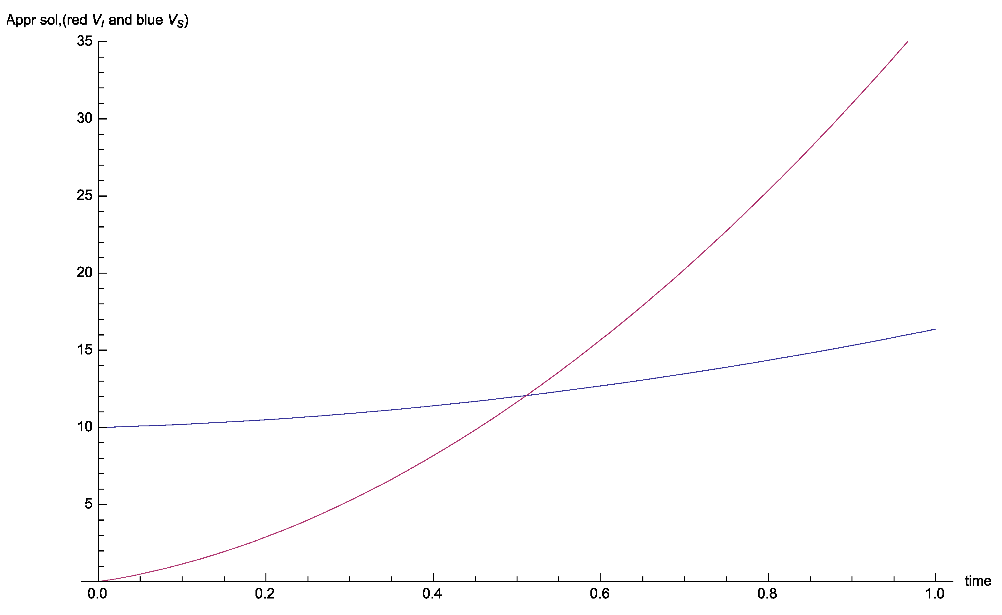
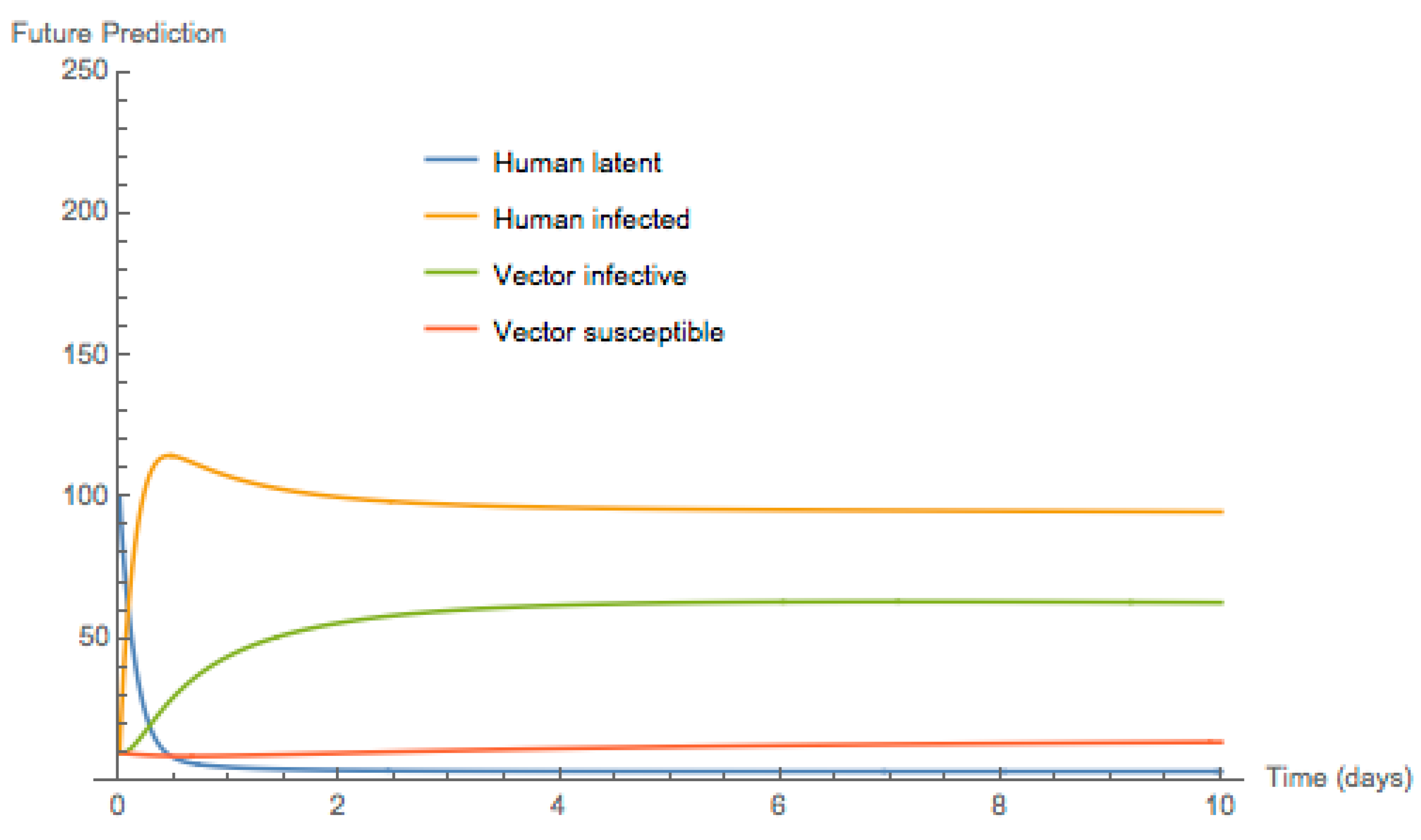
Figure 2. Approximate solution for alpha = 0.106.

Figure 2. Approximate solution for alpha = 0.106.

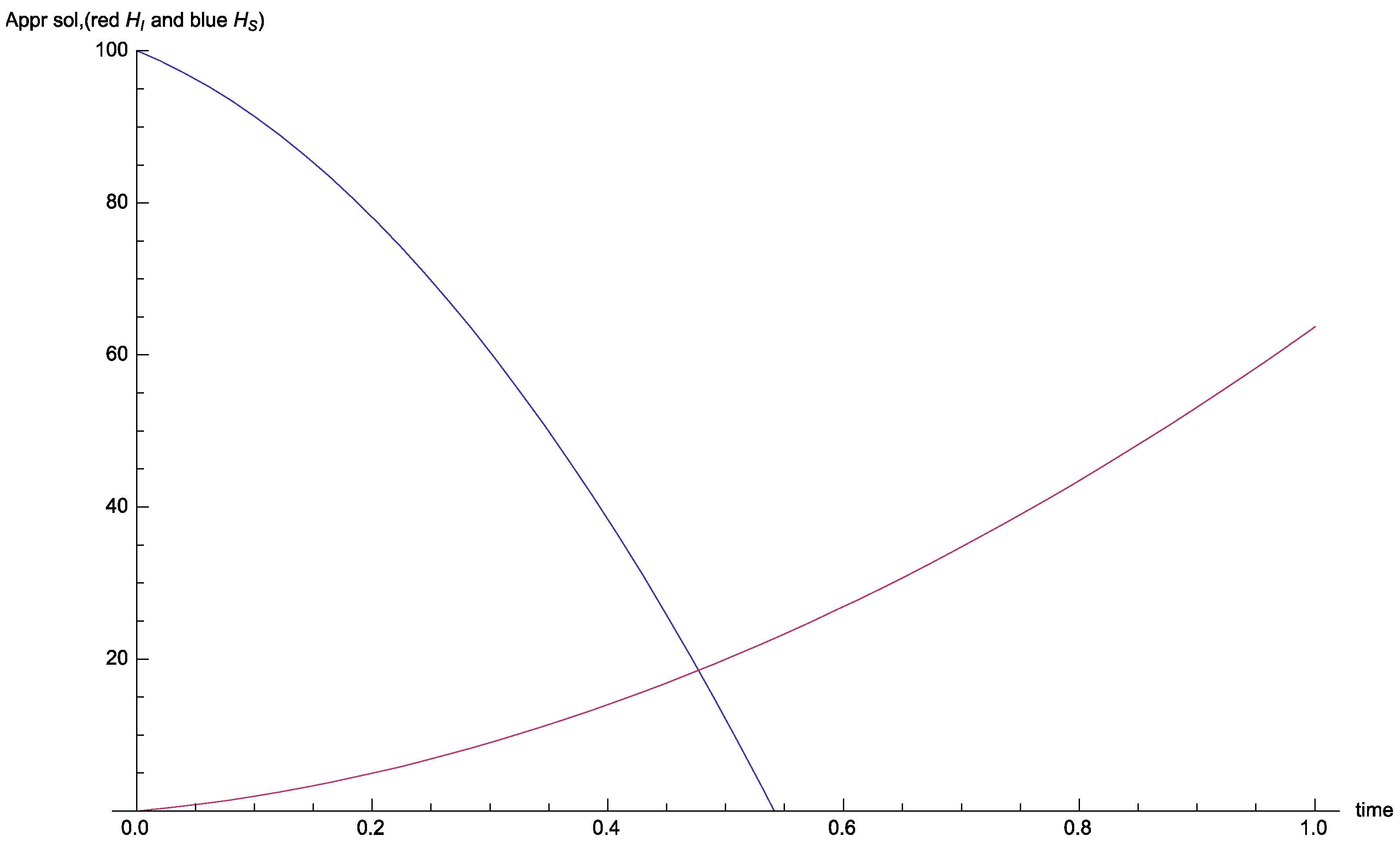
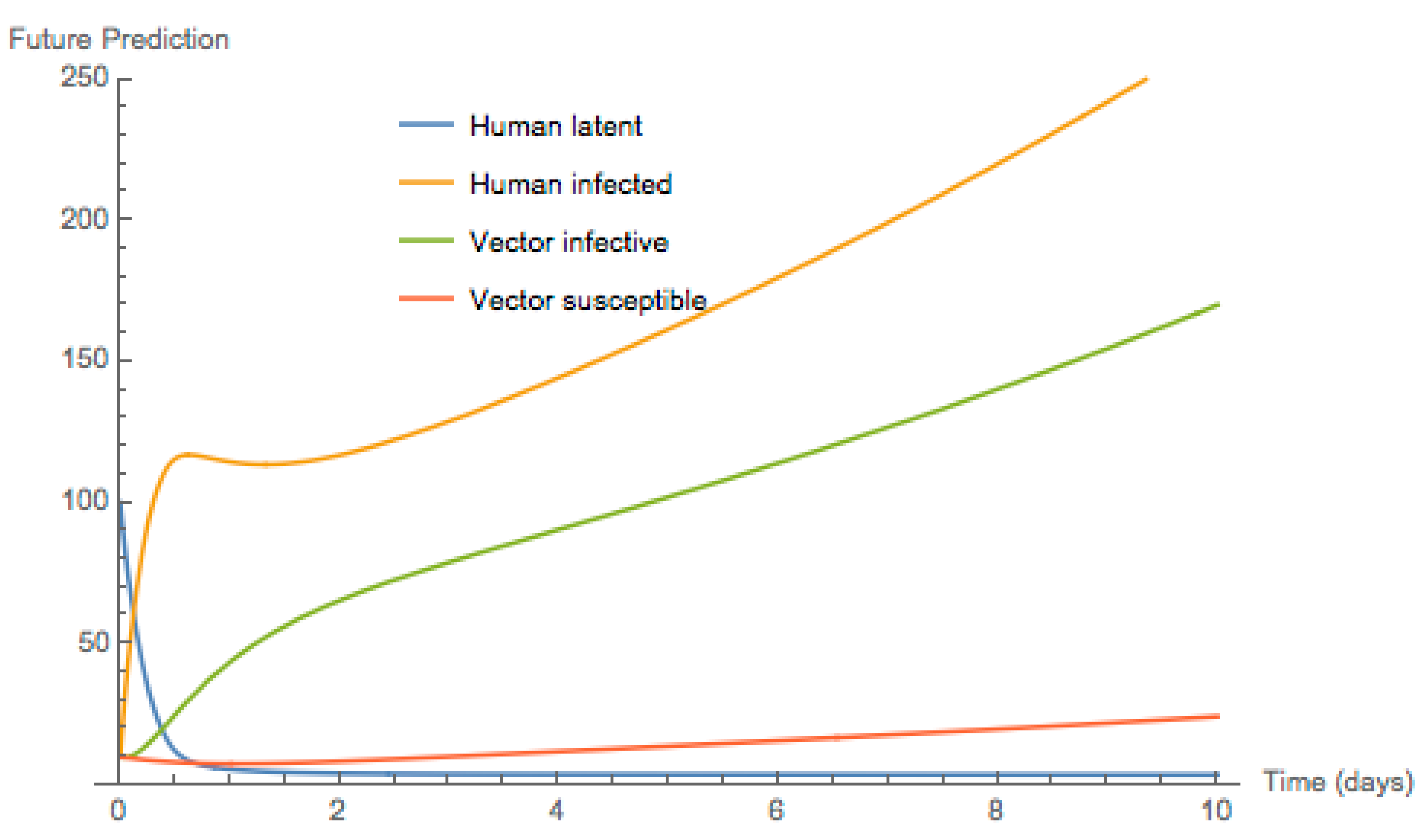
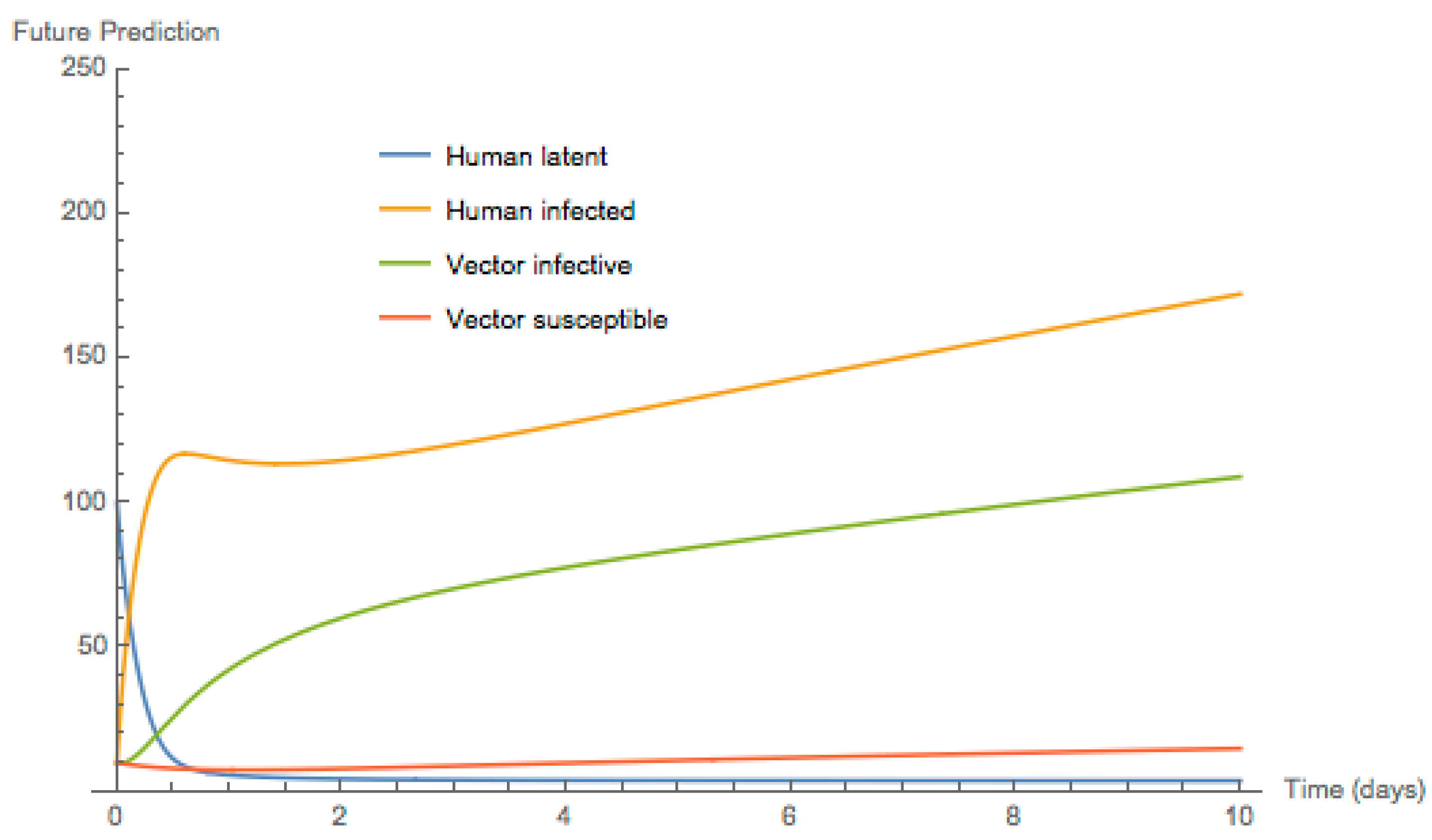
The graphical representations are depicted in Figure 2, Figure 3, Figure 4, Figure 5, Figure 6 and Figure 7. It is observed from the graph that, for the above theoretical parameters, the total population referred here as susceptible will get the disease because of the fast spread of the infection that affects almost all the people. It is also observed that, in a very short period of time, the number of infected persons will increase very rapidly. In general the number of susceptible vectors will also be described and the number of infected vectors will increase, which is actually physically normal. The results from the figure show that the prediction also depends on the fractional order mu. More precisely, when mu is closer to 1 and above 0.5, we have a non-realistic prediction, since we assume the initial number of people in the susceptible population to be 100 and also at the beginning of the infection, we assume to have 10 people that at that time were not susceptible. However, we have that, for mu above 0.5, we observe that, the number of humans infected is more than 110 and can even be 250. On the other hand, when mu is less than 0.5 the maximum number of infected human will be 110 which is very realistic because we will assume that at a particular time, the remaining 10 non-susceptible population became susceptible and later get infected. It is perhaps important to mention that, when mu is 1 we have the ordinary derivative in both cases for the beta-derivative and also the Caputo derivative, meaning the model with an ordinary derivative does not give good prediction, however with the newly introduced beta-calculus we have possibility of describing this physical problem more accurately.

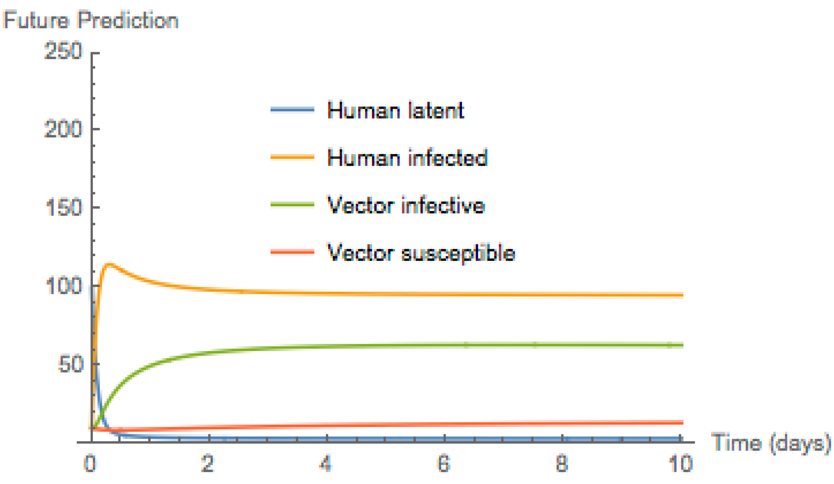
Figure 3. Approximate solution for alpha = 0.106.

Figure 3. Approximate solution for alpha = 0.106.

Figure 4. Approximate solution for mu = 1.

Figure 4. Approximate solution for mu = 1.

Figure 5. Approximate solution for mu =0.6.

Figure 5. Approximate solution for mu =0.6.

Figure 6. Approximation for mu = 0.4.

Figure 6. Approximation for mu = 0.4.

Figure 7. Approximate solution for mu = 0.25.

Figure 7. Approximate solution for mu = 0.25.

6. Conclusions

Within the help of the Caputo fractional derivative and beta-derivative, the spread of the tropical disease called onchocerciasis was investigated. This disease is found in particular in Centre and West African countries, where there are abundant rivers. We shall first note that the definition of the concept of fractional derivative is designed with the convolution of the derivative of a function together with the function power. The concept of convolution is used in many branches of science and engineering because of its properties. For instance in image processing we have the use of convolution as a filter. However, in the case of epidemiology, fractional derivatives are used for memory, the model is able to give memory of the spread from the genesis to the infected person. However using the concept of beta derivative which is the medium between fractional order and local derivative, we are able to describe the spread at a given point with a particular fractional order. In this work, we made use of two different concepts of derivative to describe the spread of river blindness disease. The modified models were solved iteratively. The results from the figures show that the prediction also depends on the fractional order mu. More precisely, when mu is closer to 1 and above 0.5, we have a non-realistic prediction, since we assume the initial number of the susceptible population to be 100 and also at the beginning of the infection, we assume the have 10 people that at that time were not susceptible. However, we have that for mu above 0.5, we observe that the number of humans infected is more than 110 and can even be 250. On the other hand, when mu is less than 0.5 the maximum number of infected humans will be 110 which is very realistic because we will assume that at a particular time, the remaining 10 non-susceptible population became susceptible and later infected. It is perhaps important to mention that, when mu is 1 we have the ordinary derivative in both case for beta-derivative and also Caputo derivative, meaning the model with an ordinary derivative does not give good prediction, however with the newly introduced beta-calculus we have possibility of describing this physical problem more accurately.

References

- Thylefors, B.; Alleman, M.M.; Twum-Danso, N.A. Operational lessons from 20 years of the Mectizan Donation Program for the control of onchocerciasis. Trop. Med. Int. Health 2008, 13, 689–696. [Google Scholar] [CrossRef] [PubMed]
- Murdoch, M.E.; Hay, R.J.; Mackenzie, C.D.; Williams, J.F.; Ghalib, H.W.; Cousens, S.; Abiose, A.; Jones, B.R. A clinical classification and grading system of the cutaneous changes in onchocerciasis. Br. J. Dermatol. 1993, 129, 260–269. [Google Scholar] [CrossRef] [PubMed]
- Murray, P.R. Medical microbiology, 7th ed.; Elsevier Saunders: Philadelphia, PA, USA, 2013; p. 792. [Google Scholar]
- Fenwick, A. The global burden of neglected tropical diseases. Public Health 2012, 126, 233–236. [Google Scholar] [CrossRef] [PubMed]
- Atangana, A.; Bildik, N. The use of fractional order derivative to predict the groundwater flow. Math. Probl. Eng. 2013. [Google Scholar] [CrossRef]
- Cloot, A.; Botha, J.F. A generalised groundwater flow equation using the concept of non-integer order derivatives. Water SA 2006, 32, 1–7. [Google Scholar] [CrossRef]
- Atangana, A.; Vermeulen, P.D. Analytical solutions of a space-time fractional derivative of groundwater flow equation. Abstr. Appl. Anal. 2014. [Google Scholar] [CrossRef]
- Su, W.; Baleanu, D.; Yang, X.; Jafari, H. Damped wave equation and dissipative wave equation in fractal strings within the local fractional variational iteration method. Fixed Point Theory Appl. 2013. [Google Scholar] [CrossRef]
- Miller, K.S.; Ross, B. An Introduction to the Fractional Calculus and Fractional Differential Equations; John Wiley & Sons: New York, NY, USA, 1993. [Google Scholar]
- Podlubny, I. Geometric and physical interpretation of fractional integration and fractional differentiation. Fract. Calc. Appl. Anal. 2002, 5, 367–386. [Google Scholar]
- Ganji, D.D.; Sadighi, A. Application of homotopy-perturbation and variational iteration methods to nonlinear heat transfer and porous media equations. J. Comput. Appl. Math. 2007, 207, 24–34. [Google Scholar] [CrossRef]
- Jibril, L.; Ibrahim, M.O. Mathematical Modeling on the CDTI Prospects for Elimination of Onchocerciasis: A Deterministic Model Approach. Res. J. Math. Stat. 2011, 3, 136–140. [Google Scholar]
- Jafari, H.; Momani, S. Solving fractional diffusion and wave equations by modified homotopy perturbation method. Phys. Lett. A 2007, 370, 388–396. [Google Scholar] [CrossRef]
- Adomian, G.; Rach, R. Analytic solution of nonlinear boundary value problems in several dimensions by decomposition. J. Math. Anal. Appl. 1993, 174, 118–137. [Google Scholar] [CrossRef]
- Wazwaz, A.M. Adomian decomposition method for a reliable treatment of the Bratu-type equations. Appl. Math. Comput. 2005, 166, 652–663. [Google Scholar] [CrossRef]
- Khan, Y. An effective modification of the Laplace decomposition method for nonlinear equations. Int. J. Nonlinear Sci. Num. Simul. 2009, 10, 1373–1376. [Google Scholar] [CrossRef]
- Singh, J.; Kumar, D.; Sushila. Homotopy perturbation Sumudu transform method for nonlinear equations. Adv. Appl. Mech. 2011, 4, 165–175. [Google Scholar]
- Atangana, A.; Bildik, N. Approximate Solution of Tuberculosis Disease Population Dynamics Model. Abstr. Appl. Anal. 2013. [Google Scholar] [CrossRef]
© 2016 by the authors; licensee MDPI, Basel, Switzerland. This article is an open access article distributed under the terms and conditions of the Creative Commons by Attribution (CC-BY) license (http://creativecommons.org/licenses/by/4.0/).